1. Introduction
Unplanned equipment failures remain a major challenge in industrial production, leading to costly downtime, quality degradation, and safety risks. In large-scale manufacturing plants, even minor malfunctions in critical rotating machinery can cascade into significant losses, as production processes are highly interconnected. Recent studies confirm this impact; Ojeda et al. [
1] demonstrated that predictive models can substantially reduce unplanned downtime in automotive production processes, while Zhao et al. [
2] highlighted the importance of prescriptive maintenance frameworks to anticipate failures and optimize resource utilization. Predictive maintenance (PdM) has therefore become a central pillar of Industry 4.0 strategies, aiming to anticipate failures before they occur and to optimize both reliability and efficiency. Recent years have seen significant advances in intelligent fault diagnosis (IFD) methods, particularly with the adoption of machine learning (ML) and deep learning (DL). These approaches enable automated extraction of discriminative features from raw vibration and operational data, outperforming traditional diagnostic methods that rely heavily on expert knowledge and manual feature engineering. Convolutional and recurrent architectures, such as Convolutional Neural Networks (CNNs) and Long Short-Term Memories (LSTMs), have demonstrated strong capability in modeling nonlinear vibration dynamics. Nevertheless, most existing studies are limited to laboratory test rigs or curated datasets, where faults are artificially induced and conditions are simplified, reducing their transferability to real-world production environments. As highlighted by Hakami et al. [
3], data scarcity and imbalance remain persistent obstacles in PdM applications, while Saeed et al. [
4] emphasize that many IFD models implicitly assume idealized data availability, which rarely reflects real industrial conditions. Similarly, Leite et al. [
5] underline that lab-scale studies often neglect practical issues such as sensor noise, varying loads, and maintenance interruptions, further constraining industrial applicability. A key challenge in this field is the scarcity and imbalance of high-quality industrial fault data. Unlike controlled laboratory benchmarks, production data rarely capture full failure trajectories, as machines are maintained or replaced before catastrophic breakdowns occur. Faults are sporadic, unevenly distributed, and intertwined with process variability, complicating model training and evaluation. These limitations highlight the need for diagnostic frameworks that can operate robustly with limited and variable fault samples while remaining applicable to real factory conditions.
Within this context, the present work focuses on centrifugal ventilators, which play a pivotal role in fiber production lines by supplying cooling air to the quenching chamber where polymer filaments are solidified. Industrial air blowers are generally used for managing airflow and temperature in various systems, with the most common types being regenerative, positive displacement, and centrifugal. Centrifugal blowers differ significantly from the others, as they are characterized by very low pressure and high airflow and operate based on impeller-driven motion [
6]. In these blowers, the air is drawn into the center of the impeller and accelerated outward by the centrifugal force generated by the rotating blades. The high-velocity airstream is collected within the blower housing, where it is converted into pressure.
Centrifugal blowers are widely used in industrial applications such as cooling, cleaning, blow-off, drying, and humidity control. Their construction includes housing, inlet and outlet ducts, a drive shaft, and a drive mechanism connected to an electrical motor. Critical to their performance are the design characteristics of the impeller blades—blade angle, length, and rotational speed—which directly affect the volume and velocity of the air flow.
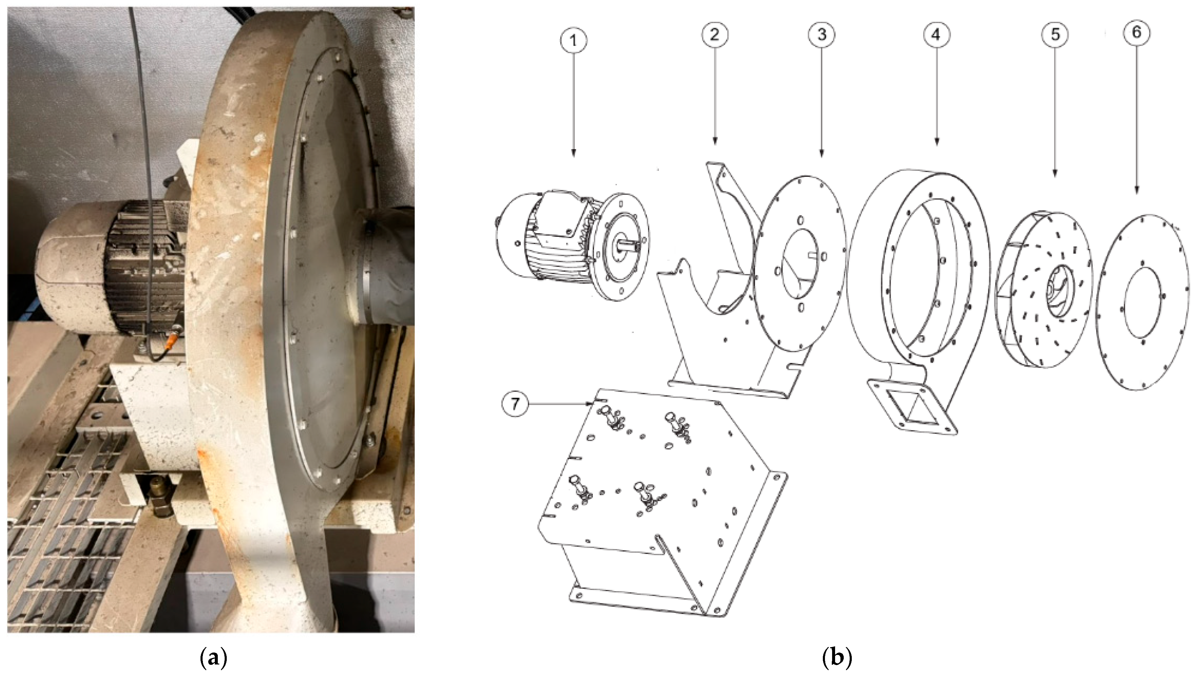
Figure 1 depicts the principal components: electric motor with the drive shaft, housing/volute with inlet and outlet ducts, impeller (fan wheel), and support frame [
7].
In the industrial application under study, these ventilators represent a critical stage (quenching) in the production process of staple fibers. The quenching system crystallizes the polymer with a cold air flow until it reaches the crystallization point. The polymer solidifies and, under constant tension, starts to stretch. After that, the yarn passes through the spin finish oil vessel for antistatic treatment, and finally it is guided to winding cylinders (spinning heads), which lead it with increasing speed to the next stage of drafting to gain specific mechanical properties [
7]. The efficiency and the uninterrupted function of the air-ventilators for cooling, is a vital factor for the quenching process in each spinning head, as even a small change in temperature during the solidifying process results in blocking of the spinneret head holes and inconsistencies in the fiber crystallization which results in bad product and even worse a lot of downtime due to more frequent cleaning of the heads and changeovers [
7]. Thus, ensuring the reliable operation of air blower systems is essential, as their performance directly impacts cooling efficiency, product quality, and overall process stability. Accurate fault diagnosis in these systems not only improves reliability and safety but also reduces maintenance costs and optimizes resource utilization. Traditional diagnostic approaches rely heavily on expert knowledge and manual feature extraction, which can be time-consuming and limited in handling the diverse vibration and operational characteristics of blower equipment. IFD using deep learning enables automatic extraction of discriminative features from raw vibration and operational data, reducing human intervention and increasing diagnostic accuracy. Nevertheless, obtaining sufficient labeled fault data under real production conditions remains challenging, highlighting the need for robust diagnostic models capable of operating effectively with limited and variable fault samples [
8].
Figure 1.
Blower’s structure: (
a) Actual operation view; (
b) Exploded view indicating provided by the manufacturers, indicating the (1) inductive motor, (2) the base, (3) the flange, (4) the housing, (5) the impeller, (6) the housing cover, and (7) the support base [
9].
Figure 1.
Blower’s structure: (
a) Actual operation view; (
b) Exploded view indicating provided by the manufacturers, indicating the (1) inductive motor, (2) the base, (3) the flange, (4) the housing, (5) the impeller, (6) the housing cover, and (7) the support base [
9].
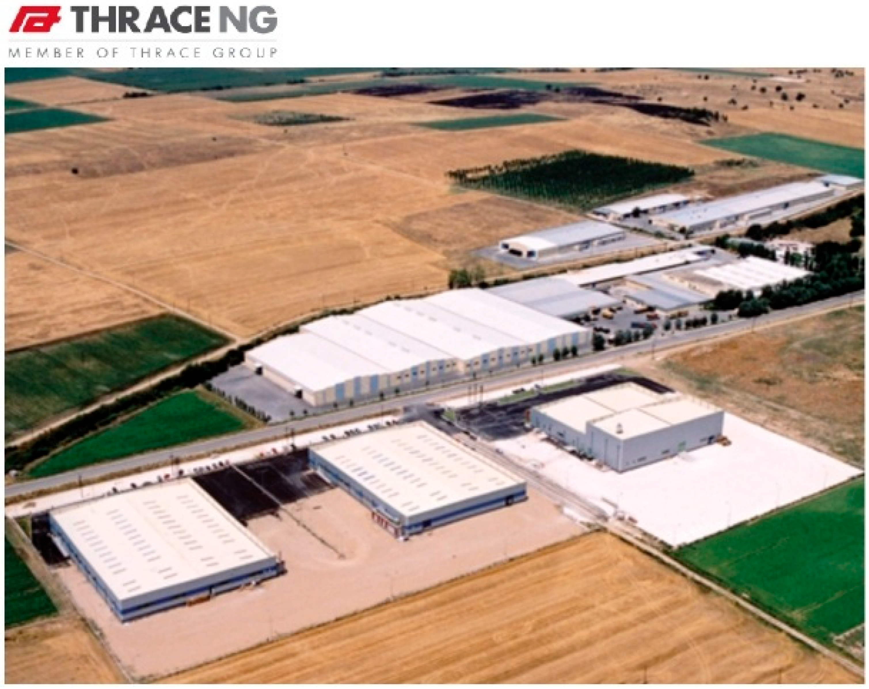
To address these challenges, this study investigates deep learning-based fault diagnosis of industrial air ventilators in a real production environment. Unlike prior research conducted on laboratory rigs or synthetic benchmarks, our work is grounded in data captured from a full-scale fiber production line at Thrace Nonwovens & Geosynthetics S.A. (Thrace NG) (
Figure 2) in Magiko, Xanthi, Greece [
10]. Thrace NG, a leading European manufacturer of nonwoven and geosynthetic products, provides an authentic industrial testbed where blower reliability is critical: even minor faults can compromise fiber quality, reduce efficiency, and trigger costly production interruptions. By situating the analysis within such a high-demand industrial setting, the proposed methodology directly reflects the operational variability, maintenance practices, and real constraints of factory-scale systems—bridging the gap between academic model development and practical industrial deployment.
Building on the need for reliable and practical predictive maintenance solutions in industrial environments, this study makes three key contributions:
- 1.
Development of an industrial multi-sensor dataset. We introduce and openly provide a curated dataset collected from centrifugal ventilators in a full-scale fiber production line. Unlike prior studies that rely on laboratory rigs or synthetic data, this dataset captures authentic process variability and is systematically aligned with maintenance events, ensuring both realism and reliability.
- 2.
Comprehensive benchmarking of diagnostic models. We conduct a systematic comparison of state-of-the-art deep learning architectures (ResNet50-1D, CNN-1D, BiLSTM, BiLSTM + Attention) against traditional baselines (Random Forest, LSTM). By employing both conventional train–test splits and rigorous cross-validation schemes, we provide a robust evaluation of model generalization under realistic industrial constraints.
- 3.
Integration into a maintenance-oriented framework. Beyond performance benchmarking, we propose a diagnostic framework that aligns predictive outputs with historical maintenance logs and translates them into a severity-based prioritization strategy. This ensures that the results are not only accurate in classification but also directly actionable within industrial maintenance planning.
Together, these contributions bridge the gap between academic model development and industrial deployment, demonstrating how DL-based fault diagnosis can be effectively adapted to the challenges of real-world production environments.
The rest of this work is structured as follows.
Section 2 reviews related works.
Section 3 presents the proposed methodology, by separating it into two distinct stages, i.e., fault diagnosis, and severity-based maintenance strategy. The experimental setup for fault diagnosis is included in
Section 4, while data curation is presented in
Section 5. The results of fault classification are summarized in
Section 6.
Section 7 presents the proposed severity-based maintenance strategy. Finally,
Section 8 and
Section 9 include the discussions and the conclusions, respectively.
2. Related Works and Contributions
DL has rapidly advanced fault diagnosis capabilities across various industrial domains. Since 2012, there has been a surge in research leveraging DL for predictive maintenance, anomaly detection, and overall equipment health monitoring [
11]. Early approaches predominantly employed shallow learning methods like Support Vector Machines (SVM), k-Nearest Neighbors (KNN), Artificial Neural Networks (ANN), and Naive Bayes [
12]. These traditional techniques required manual feature extraction and were often constrained in handling high-dimensional or non-linear data. The advent of deep architectures such as Convolutional Neural Networks (CNNs), Autoencoders (AEs), Deep Belief Networks (DBNs), and Recurrent Neural Networks (RNNs) transformed the field by enabling automatic, hierarchical feature extraction and superior classification accuracy, particularly when applied to large datasets [
13]. Recent reviews further emphasize this transformation, noting that DL is now the dominant paradigm in machinery health management, but practical deployments remain scarce [
4,
5].
Among DL models, CNNs have been prominently utilized for diagnosing faults in rotating machinery, bearings, and gears [
14,
15,
16,
17]. Their ability to extract spatial and spectral features from raw vibration signals, time-frequency images, infrared thermal images, and other sensor modalities has led to enhanced fault identification performance. Techniques such as wavelet regularization [
18], data augmentation [
19], and information fusion [
20] have further bolstered CNN robustness. Transfer learning and domain adaptation strategies have improved CNN generalization across varying equipment and operating conditions [
21,
22]. To address class imbalance, Generative Adversarial Networks (GANs) have been combined with CNNs to synthetically generate underrepresented fault cases [
23,
24]. Complementary to such synthetic approaches, Hakami et al. [
3] demonstrated that imbalance and scarcity are structural properties of industrial data, requiring tailored solutions rather than preprocessing fixes. Similarly, Zhao et al. [
2] introduced a transformer-driven prescriptive maintenance framework, namely TranDRL, highlighting how newer architectures can extend predictive maintenance beyond fault detection into decision support.
In real manufacturing settings, curating balanced fault datasets is intrinsically difficult. Production lines run under continuously varying regimes (load, speed, temperature, product grade), while genuine faults occur sporadically, non-uniformly, and often idiosyncratically to specific maintenance and operating contexts. Safety, quality, and uptime constraints preclude inducing failures on demand, and labeling is labor-intensive during short downtime windows; consequently, normal operating data dominate, and several fault categories remain severely underrepresented. This class skew biases learning toward majority behaviors, inflates false negatives for rare failures, and undermines generalization across operating conditions. As emphasized by Sun et al. (2024) [
25], in practical engineering it is “extremely difficult to obtain enough labeled fault samples,” leading to datasets where normal data predominate and faults are scarce; they further document that diagnostic accuracy degrades as the imbalance ratio worsens, underscoring how dataset imbalance is a structural property of industrial data rather than a curable preprocessing artifact. This observation aligns with Saeed et al. [
4], who noted that many IFD models implicitly assume idealized data availability, which rarely reflects production reality.
Concerning air blowers and ventilation applications, fault diagnosis has become a vital area of research due to the critical role these components play in industrial ventilation and cooling systems. Studies in this domain have progressively adopted advanced techniques combining signal processing and intelligent algorithms to detect and classify faults, often to enable predictive maintenance and avoid production interruptions [
26,
27]. Wu and Liao [
28] developed a diagnostic system for automotive air-conditioning blowers using Empirical Mode Decomposition (EMD) and a Probabilistic Neural Network (PNN). Their method proved more accurate and computationally efficient than conventional back-propagation networks, especially in handling nonlinear and non-stationary signals. Ma et al. [
29] applied Wavelet Envelope Spectrum Analysis combined with Hilbert transforms to identify early signs of rotating stall in catalytic cracking unit blowers. Their approach effectively isolated critical frequency components under transient conditions, enabling timely fault detection. Li and Yang [
30] proposed a hybrid diagnostic model using Genetic Fuzzy Neural Networks (GFNN), which leveraged fuzzy logic and genetic algorithms to enhance fault classification accuracy and convergence rate. Their system showed resilience across various types of mechanical anomalies. Zheng et al. [
31] studied magnetically suspended blowers and introduced a cross-feedback control model to mitigate rotor nutation vibrations. The method achieved a 50% reduction in vibration amplitude, improving stability during high-speed operation. Salem et al. [
26] conducted multiple investigations into forced blower fault prediction using vibration data. In their study, they employed machine learning models including Multilayer Perceptron (MLP), XGBoost, and hybrid classifiers. Results demonstrated high diagnostic accuracy, with XGBoost consistently outperforming alternatives in precision and robustness. Karapalidou et al. [
32] utilized DL to develop stacked sparse Long Short-Term Memory (LSTM) autoencoders for anomaly detection in industrial blower bearing units. Using only healthy operational data for training, their models accurately identified anomalies in encumbered states and generalized well to other equipment. Qin et al. [
33] combined Multi-Scale Dimensionless Indicators (MSDI), Variational Mode Decomposition (VMD), and Random Forests to diagnose faults in centrifugal blowers, achieving a classification accuracy of 95.58%. Their method underscored the value of multi-scale feature extraction and ensemble learning in dynamic systems. Liu et al. [
34] applied improved neural network models to evaluate blower health using spindle speed and power output as key indicators. Fordal et al. [
35] contributed to predictive maintenance frameworks using ANNs and sensor-based platforms, offering scalable solutions compatible with Industry 4.0 infrastructures. More recent works expand the scope beyond blowers: Ojeda et al. [
1] demonstrated PdM models reducing downtime in automotive production, while Poland et al. [
36] proposed transformer-based prognosis for general industrial machines. Both highlight the trend toward broader industrial deployment of PdM, though not specifically targeting ventilators.
Collectively, these studies underscore the importance of DL architectures (e.g., LSTM autoencoders, stacked networks), hybrid models combining traditional ML with advanced feature extraction, and real-world implementation of fault diagnosis and maintenance models on industrial ventilation applications using air blowers. However, related works mainly rely on lab-controlled or simulated data, which limits their scalability and real-time industrial deployment.
In contrast to related works on industrial fault diagnosis, which often rely on simulated datasets and synthetic fault data augmentation techniques, laboratory-scale machinery, or single-type models, this work conducts DL-based fault detection in an actual running industrial production setting with limited fault sample data in comparison with the normal data. It should be noted that DL-based fault detection of air ventilators on actual fiber yarn production lines is not reported in the literature. Moreover, the proposed approach uses and distributes openly real-time sensor data, and correlates equipment diagnosis and maintenance scheduling with historical maintenance logging, thereby bridging the gap between theoretical model performance and practical maintenance planning. The industrial system used in this work operates under real production variability, including changes in speed, load, and operating conditions, and supports maintenance through severity-based fault prioritization derived directly from field operations. This makes our research framework both immediately actionable and highly relevant for production-level deployment, addressing a critical gap in existing literature.
To provide a structured overview,
Table 1 summarizes representative related works, outlining their contributions, limitations, data sources, and applied models, together with a direct comparison to the present study. This consolidated view highlights the distinctive aspects of our framework and clarifies how it addresses gaps left by prior research.
3. Proposed Methodology
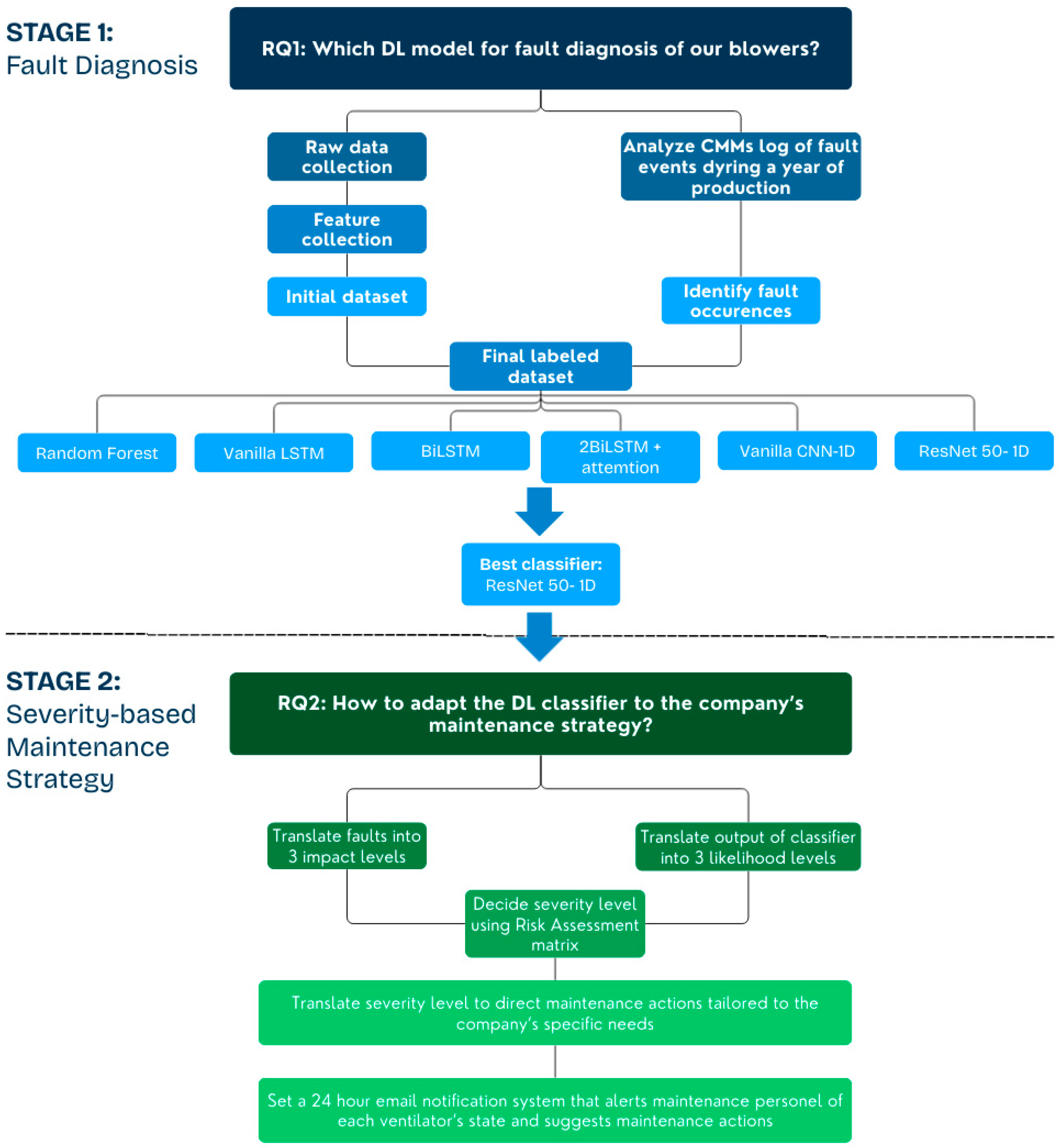
This study adopts a two-stage research methodology, aiming to fulfill two main scopes: (1) to develop a robust DL-based fault diagnosis model for industrial blowers, and (2) to integrate the model’s outputs into a practical, severity-based maintenance strategy tailored to the operational context of the company. The research methodology roadmap is illustrated in
Figure 3.
At each stage of the methodology, a research question (RQ) is answered:
Stage 1: Fault Diagnosis.
RQ1: Which deep learning model provides the most effective fault diagnosis for our industrial blowers?
Stage 2: Severity-Based Maintenance Strategy.
RQ2: How can the selected DL classifier be integrated into the company’s maintenance strategy?
3.1. Stage 1: Fault Diagnosis
For fault detection, the methodology begins with the construction of a labeled dataset integrating both sensor-derived and log-based information systems (CMMs). The final dataset is then used to train a set of selected classification models, including both traditional machine learning (ML) and DL architectures:
Random Forest (ML model used as reference)
Vanilla Long Short-Term Memory (LSTM)
Bidirectional LSTM (BiLSTM)
BiLSTM with Attention Mechanism
Vanilla Convolutional Neural Network 1D (CNN-1D)
ResNet50-1D
Evaluation of multiple models for industrial fault diagnosis is perused, since each model brings unique strengths to the task of detecting and classifying faults in complex machinery and systems.
Random Forest is used as a reference ML model. It is known as a strong baseline model that is robust and interpretable. It performs well on tabular datasets and can handle non-sequential fault patterns effectively [
37].
LSTMs are suitable for time-series data since they excel in capturing long-term dependencies in fault progression. The latter is useful for early fault detection [
38]. BiLSTM improves upon vanilla LSTM by analyzing sequences in both forward and backward directions. Thus, it is ensured that future states also contribute to fault detection accuracy [
39]. BiLSTM with an attention mechanism further enhances BiLSTM by assigning importance weights to different time steps. This aims towards focusing on the most relevant information in diagnosing faults dynamically.
CNN-1D is well-known for its effectiveness in the extraction of local patterns from sensor data, which is useful for identifying localized anomalies in industrial systems [
40]. Unlike LSTM-based variations, which capture temporal dependencies, CNNs excel at extracting spatial patterns from input features, making them particularly effective for feature learning and noise reduction in time-series data. By transitioning to a CNN-based approach, the goal is to evaluate whether deep feature extraction through convolutions can improve fault detection performance and possibly reduce misclassification rates compared to LSTMs, which rely heavily on sequential dependencies. While CNN-1D effectively extracts spatial patterns, it can struggle with deep feature learning, especially when dealing with complex fault patterns that require deeper networks.
ResNet50-1D is a deep CNN architecture that utilizes residual learning, allowing for deeper feature extraction without degradation, which could lead to improved accuracy in complex fault classification tasks [
41].
These models were chosen based on their reported results, aiming to evaluate their performance for the problem under study by covering a wide range of factors like dataset structure, fault complexity, and the need for interpretability versus high accuracy. The models were parameterized and evaluated using standard classification metrics, with emphasis on accuracy, precision, recall, and confusion matrix analysis. ResNet50-1D architecture demonstrated the highest overall performance and was selected as the preferred model for deployment, referring to the second stage of the methodology.
3.2. Stage 2: Severity-Based Maintenance Strategy
In order to provide a severity-based maintenance strategy for the company, the outputs of the best performing DL classifier (ResNet50-1D) were embedded into a structured maintenance decision-making framework that translates fault predictions into actionable insights.
To estimate maintenance urgency and guide appropriate actions, the model outputs were mapped into a risk matrix based on two dimensions:
Impact Assessment: Each fault type was classified into one of three impact levels.
Likelihood Estimation: The classifier’s probabilistic output was translated into three discrete likelihood categories, indicating a predicted probability of fault occurrence.
Combining these two axles enabled the estimation of a severity level using a risk assessment matrix commonly employed in industrial safety and reliability engineering. Next, using the Computerized Maintenance Management Systems (CMMS) database, combined with the maintenance team’s knowledge base and experience, the computed severity levels were translated into maintenance directives specifically designed to align with the company’s maintenance capabilities, resource constraints, and operational priorities.
Finally, to ensure real-time responsiveness, a 24-h automated email notification system was developed. This system continuously monitors blower conditions, interprets fault likelihoods and severities, and dispatches timely alerts to maintenance personnel. Notifications include fault type, severity level, and recommended maintenance actions, thereby facilitating proactive and targeted interventions.
4. Experimental Setup
In this section, the experimental setup is described, including the specific equipment, hardware and network connectivity utilized for capturing the vibration data.
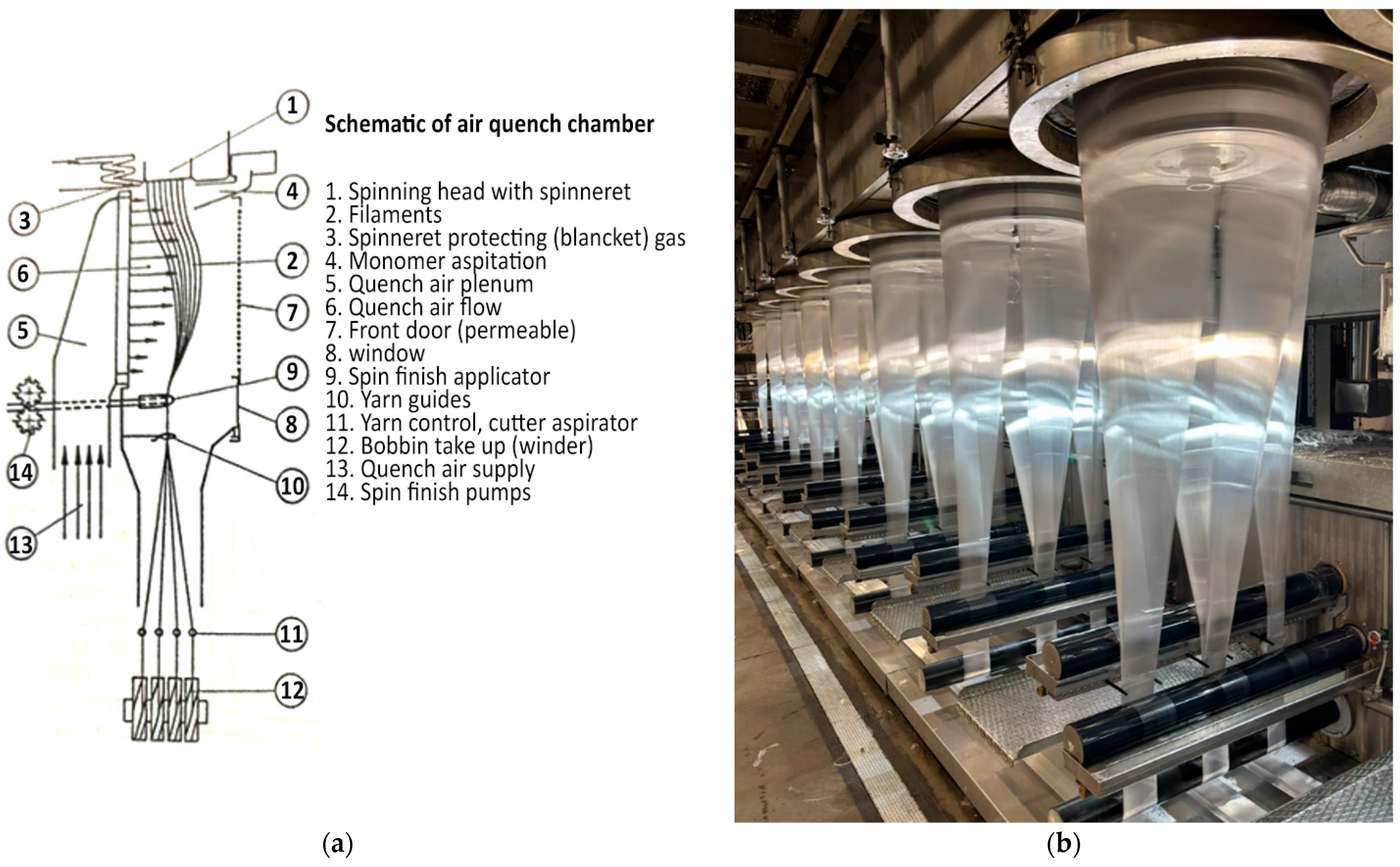
The air quenching chamber schematic is provided in
Figure 4a. With reference to
Figure 4a, the extruded hot polymer material enters a set of Spinning heads (part 1) to turn into solid filaments called yarns (part 2). The number of yarns that exit each head depends on the number of holes on each head and changes based on the product specification. In between the solidifying of the material into yarns, a quenching chamber (parts 5 and 6) is taking place, which is constantly supplied with cold air from an air-ventilator (part 13).
In
Figure 4b, the production process of fiber yarns from 10 spinning heads in real-time is shown.
4.1. Sensors
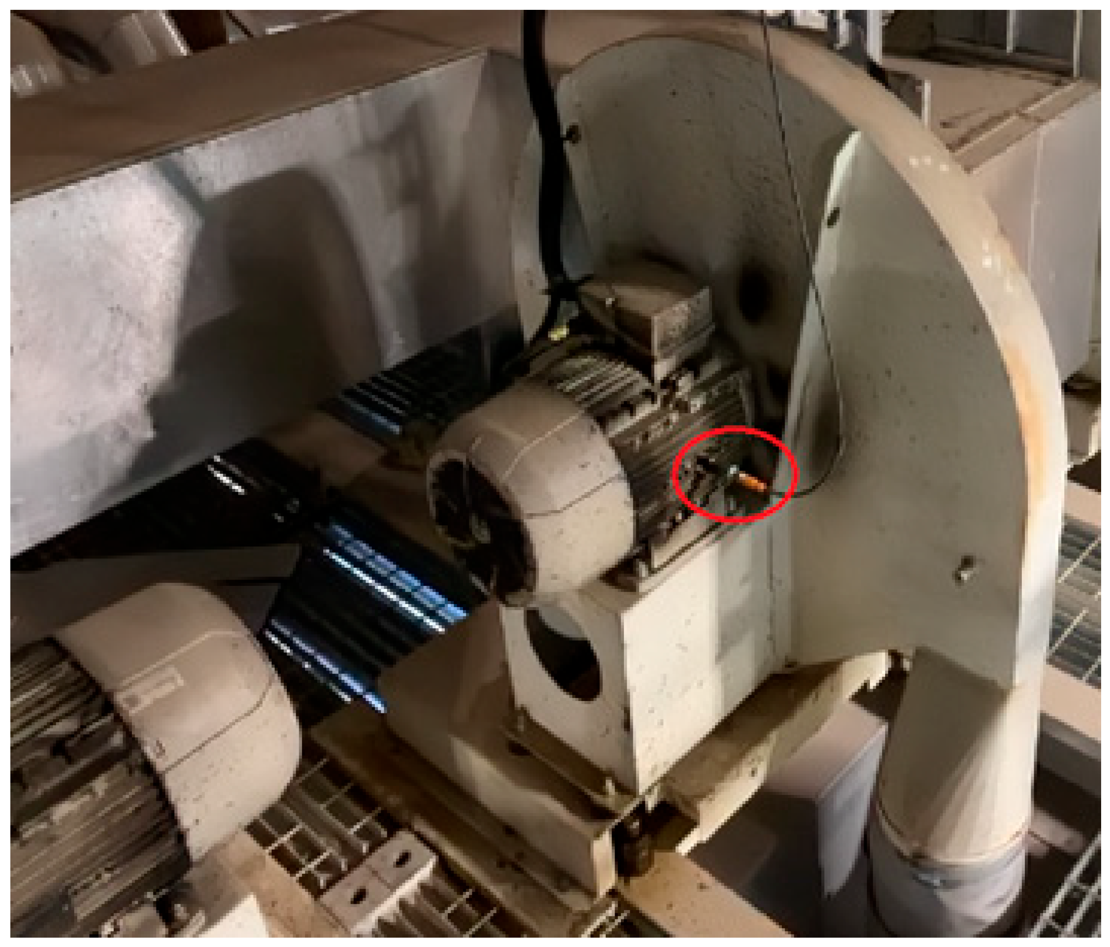
At the beginning of 2024, 10 IFM VVB001 vibration sensors were installed on ten 7.5 KW ventilator motors of the Fiber production line at one of the factories of Thrace NG. The VVB001 accelerometers are screw-mounted radially to the rotation axis of the motors. Also, according to the manufacturer’s direction, they are installed at a distance less than 50 cm from all the objects to be monitored (bearing, impeller, motor shaft, etc.) [
42], as shown in
Figure 5.
4.2. Connectivity
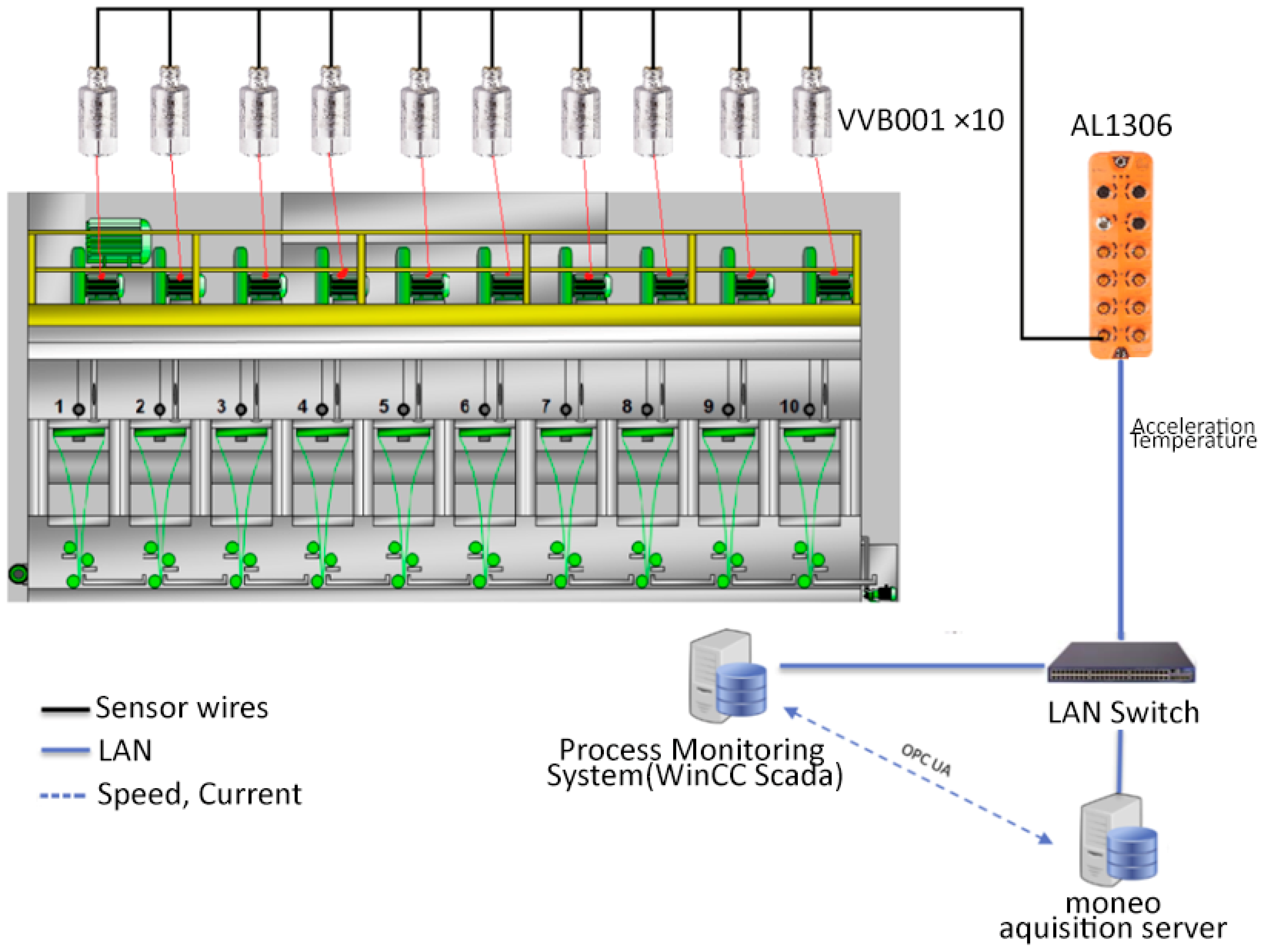
The VVB001 sensors communicate via the IO-Link protocol and digitally transmit real-time data to the IO-Link master unit AL1306.
The IO-Link master unit AL1306 collects data from the sensors and transmits it via Modbus TCP to the moneo IIoT platform, an application that manages, records, and visualizes sensor data.
The moneo IIoT platform, through its OPC-UA protocol, enables bidirectional communication with the WinCC-SCADA process monitoring system, which:
Sends motor speed and operating current to the moneo IIoT platform for data analysis.
Receives the characteristic values v-RMS, a-RMS, a-Peak, Crest, Temperature and Current from the moneo IIoT platform for storage in its database.
The WinCC-SCADA process monitoring system logs data using the Data Logging mechanism, storing values every minute in its database.
Then, the data are transferred to the Process Historian via Microsoft Message Queuing (MSMQ), which:
Continuously stores measurements, applying data compression to manage large volumes of information.
Generates daily reports (Excel Reports) for further analysis.
Figure 6 illustrates the input/output (I/O) connectivity that is described and required to collect and manage the storage of the vibration data.
5. Data Capturing and Processing
In this section, the whole process from capturing the asynchronous transmission of raw data from the mounted sensors to forming the final datasets for training the six classification models is described.
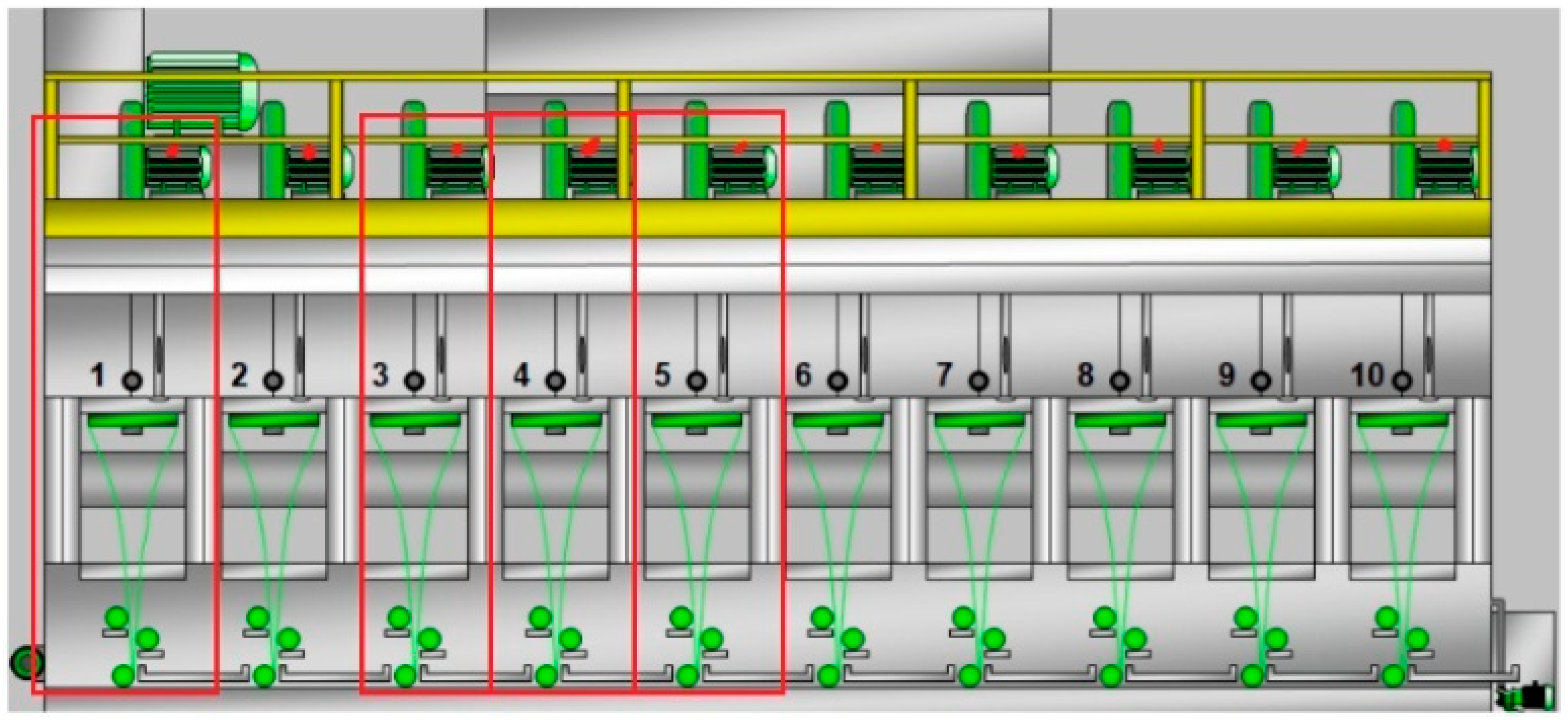
After reviewing the maintenance log of the company regarding all the reported faults that happened on the ten ventilators from early 2024 and within a period of nine months, we identified in total five repeating fault events (three fault classes) in a total of four ventilators. Thus, these four ventilators (ventilators 1, 3, 4 and 5) are being chosen as subjects for our diagnosis models. In
Figure 7, the four chosen ventilators are marked in red.
5.1. Data
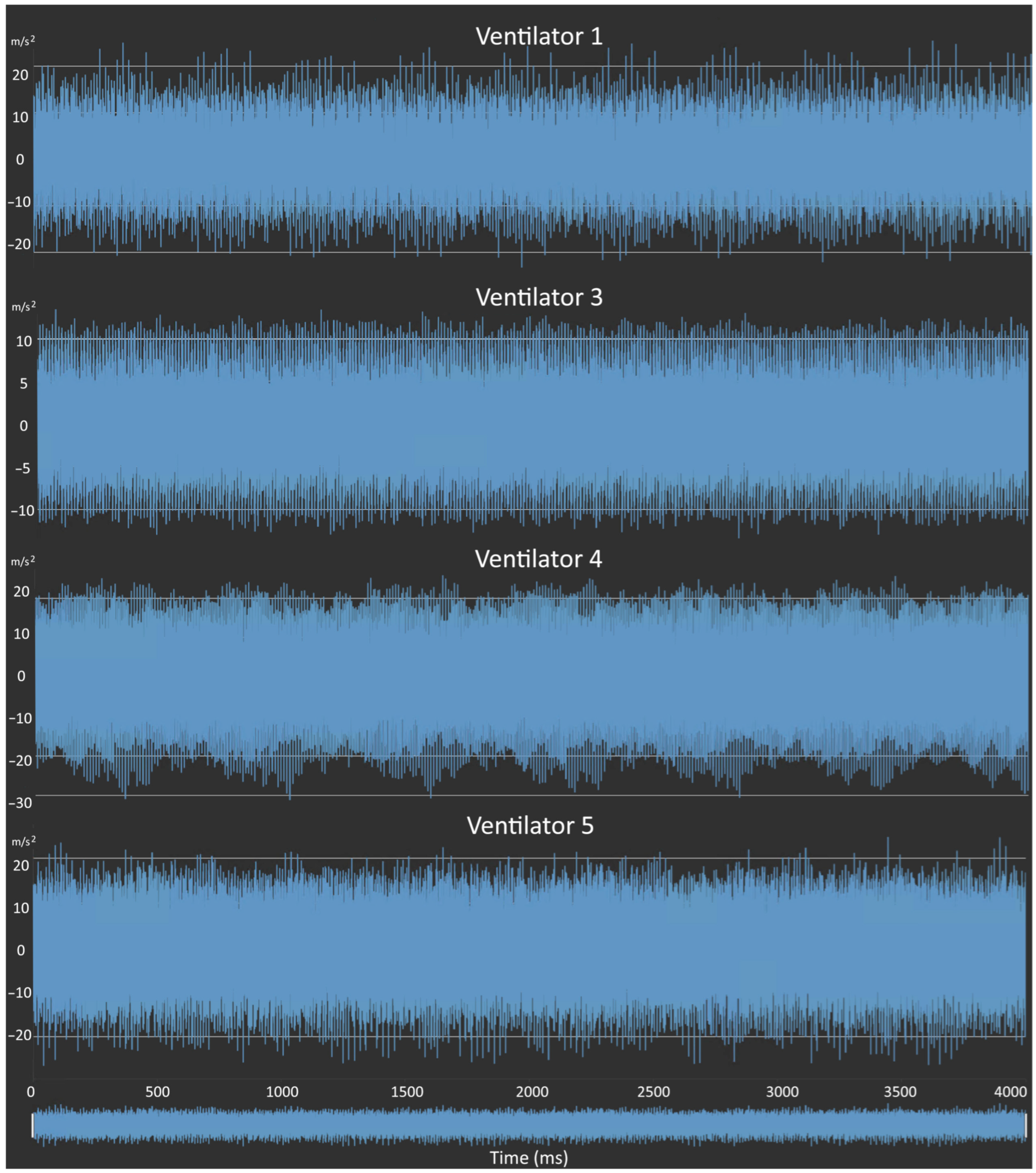
Raw data refers to vibration acceleration data with 4 s collection frequency (25 kHz) captured from the four ventilator motors, as shown in
Figure 8. The period of collection corresponds to actual production runs in the span of nine months, cumulatively for the four ventilator motors. In this period, a total of three distinctive repeating faults were identified (Impeller fault, Bearing fault, and Support cracking) in four ventilating motors and fixed at the arranged stoppages of the production. In this production line, preventive maintenance stops are performed only on product changes due to the long downtime for the changeover of the Spinneret heads. Based on the latter, we set a total of five distinctive production runs that correspond to the respective three repeated faults that were diagnosed and repaired by the production and technical teams during these changeovers.
5.2. Features
Two categories of four vibrations and three motor features are collected. First, we define the vibration features that are collected from the VVB001 sensors. These sensors are an integrated system that captures the raw vibration data and simultaneously through the moneo software (version 1.16) interface provides the ability to set the detection of the characteristic values of vRMS, aRMS, aPeak and Crest.
The characteristic value vRMS represents the vibration velocity and determines the energy acting on the machine. Its increase can be caused by low-frequency fault conditions. The most common causes include misalignment, imbalance, belt transmission issues, loose machine footing, and structural problems. Mechanical impact (aPeak) and friction (aRMS) are two parameters related to the peak acceleration values of vibrations and their root mean square acceleration values. Bearing damage, friction, impact, and cavitation cause high-frequency and low-energy vibrations, especially in the early stages of a problem. These are not covered within the low-frequency range and do not affect the vRMS value until they reach a more advanced stage. In this case, the peak value and the RMS value of vibration acceleration are particularly useful because they change at an earlier stage, allowing the identification of these issues.
The Crest Factor (CF) is a crucial feature in vibration analysis, as it helps detect early-stage faults, impact loads, and transient stress peaks in rotating machinery. Defined as the ratio of the peak amplitude to the RMS value of a vibration signal, it is particularly sensitive to short-duration impulses caused by bearing defects, gear wear, and cracks. Unlike RMS, which averages the signal and can mask transient events, a high Crest Factor indicates sharp impacts that may suggest structural issues or lubrication problems. Monitoring CF trends over time allows for predictive maintenance, as an increasing CF suggests worsening conditions that require inspection. Since CF is dimensionless, it can be applied across various machinery types for fault classification.
The second group of the three motor features consists of the current, temperature and motor’s rotation speed. These features are indicative of electrical problems or increased friction due to excessive load, insufficient lubrication, and mechanical component wear. Motor rotation speed is a vital feature that enables the DL model to be trained properly on different frequency ranges and be able to distinguish Normal and Fault states at different frequency rates. Therefore, the seven features used in this work are: vRMS, aRMS, aPeak, Crest, Temperature, Current, and Speed.
The moneo software interface developed by Integrated Facilities Management (IFM), was utilized to configure the extraction of the four vibration features aggregated to 1-min intervals from the raw acceleration data. In addition, the installed sensor has an integrated temperature probe, which provides 1-min aggregated temperature values as well. Finally, the software provides an OPCUA communication protocol that enables us to collect minute process data (motor current and variable speed) through the WINCC SCADA system. After collecting the final csv files of the five production runs with respect to the seven features, the final data frames for the model training are created.
5.3. Labeling
The final datasets of the features are analyzed and cross-examined with the Maintenance logs system of the company to label the normal and faulty data. The company uses Computerized Maintenance Management software (CMMs) Coswin 8i version 8.9 to manage their maintenance operations. This database provides valuable information to support maintenance workers to perform their tasks effectively and provides useful insight into management to make informed decisions. (e.g., calculate benefit/cost for machine breakdown versus preventive maintenance and allocate stoppages and resources accordingly.
We used this software to identify and label all possible faults regarding the four Ventilators. The labeling methodology we used is based on the records entered by the technical personnel, starting from the first report of each fault detection in the CMMS and continuing through to the final entry documenting its inspection and repair. More specifically, in
Figure 9, a snapshot of this analysis is illustrated, in which we labeled the fault on ventilator 1. On the CMMs system interface, we first identified the first entry of reporting any need for inspection on the ventilator 4, until the last entry of the scheduled inspection and repair. We also discussed with the technical department to gather more intel on the fault. In the specific case of the CMMs snapshot of
Figure 9, a report on noise on ventilator 1 was registered by the morning shift leader on the 8th of July, and the technical department scheduled an inspection on the nearest scheduled change-over stoppage on the 22nd of July. During inspection, the technical supervisor logged onto the system that the outer ring of the ventilator 1 motor’s front bearing was broken and replaced it. This simple but hectic methodology was followed to identify and label all the fault events on the four ventilators.
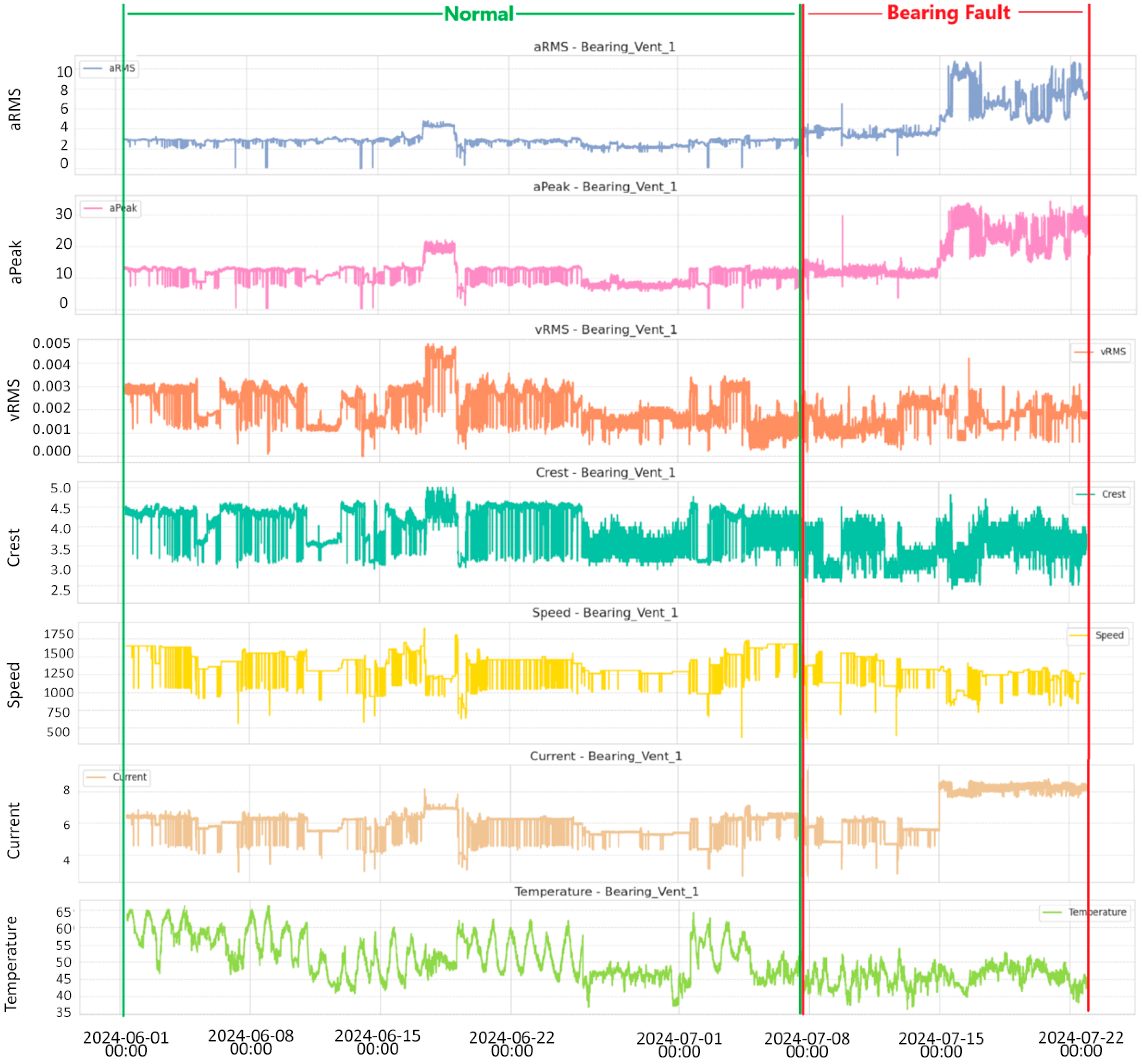
The next step after identifying all the faults and fixes/replacement events for the 4 ventilators, was to capture and export all the 1 min. vibration and motor features for each run that leads to each event. A total of about 1 month of ventilator running until the maintenance and fault identification were captured for each. Following this, a careful analysis of the final feature graphs was conducted in cooperation with the experienced maintenance team to finalize the labeling of the “normal” and “faulty” timestamps. In
Figure 10, the process of collecting Normal and Fault Timestamps is depicted in the case of a faulty bearing on ventilator 1.
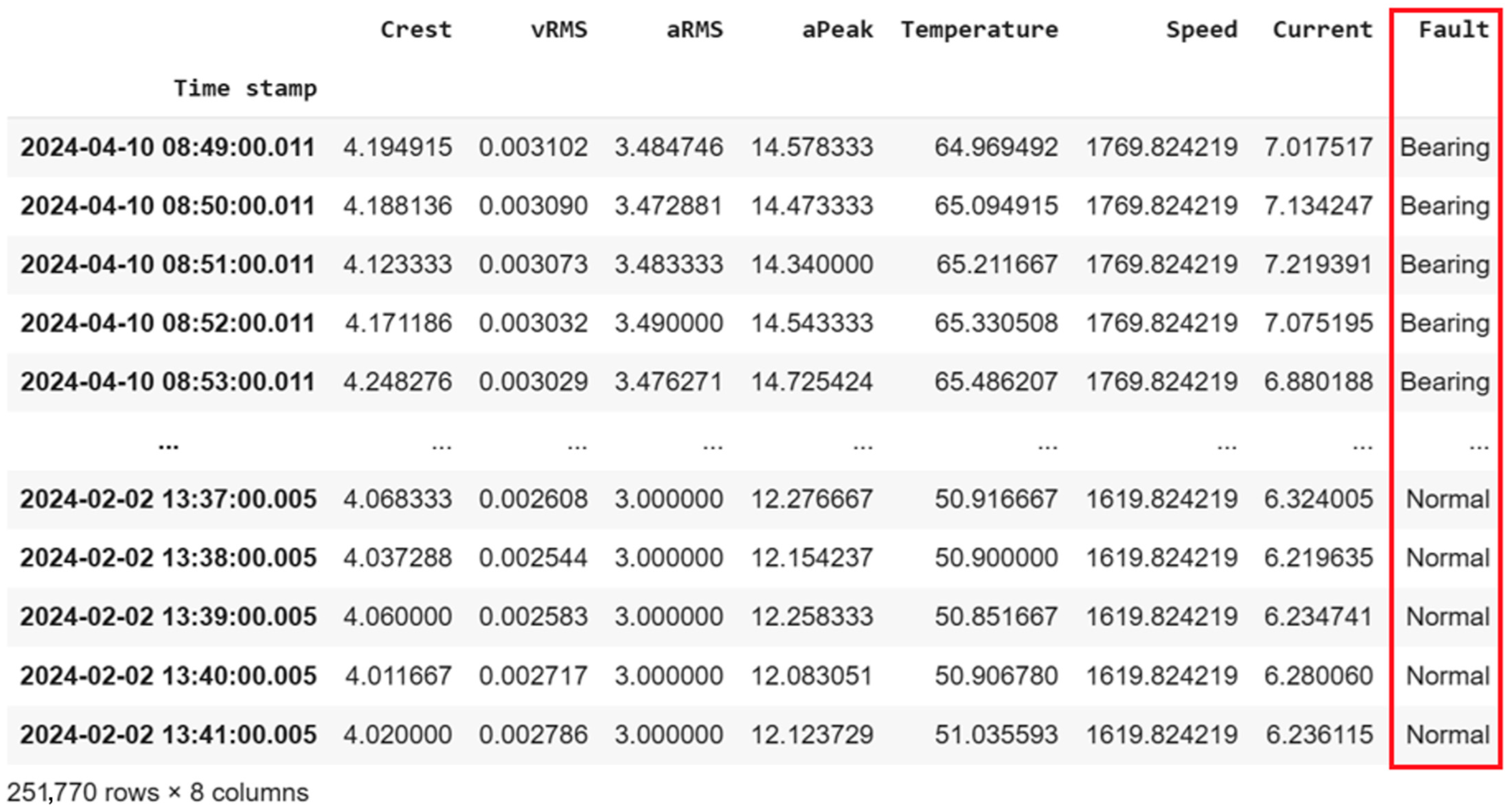
By repeating this process for the rest of the faulty events, we eventually created a final concerted data frame with all the labels in the last column, as shown in
Figure 11, ready to be used for training the classification models.
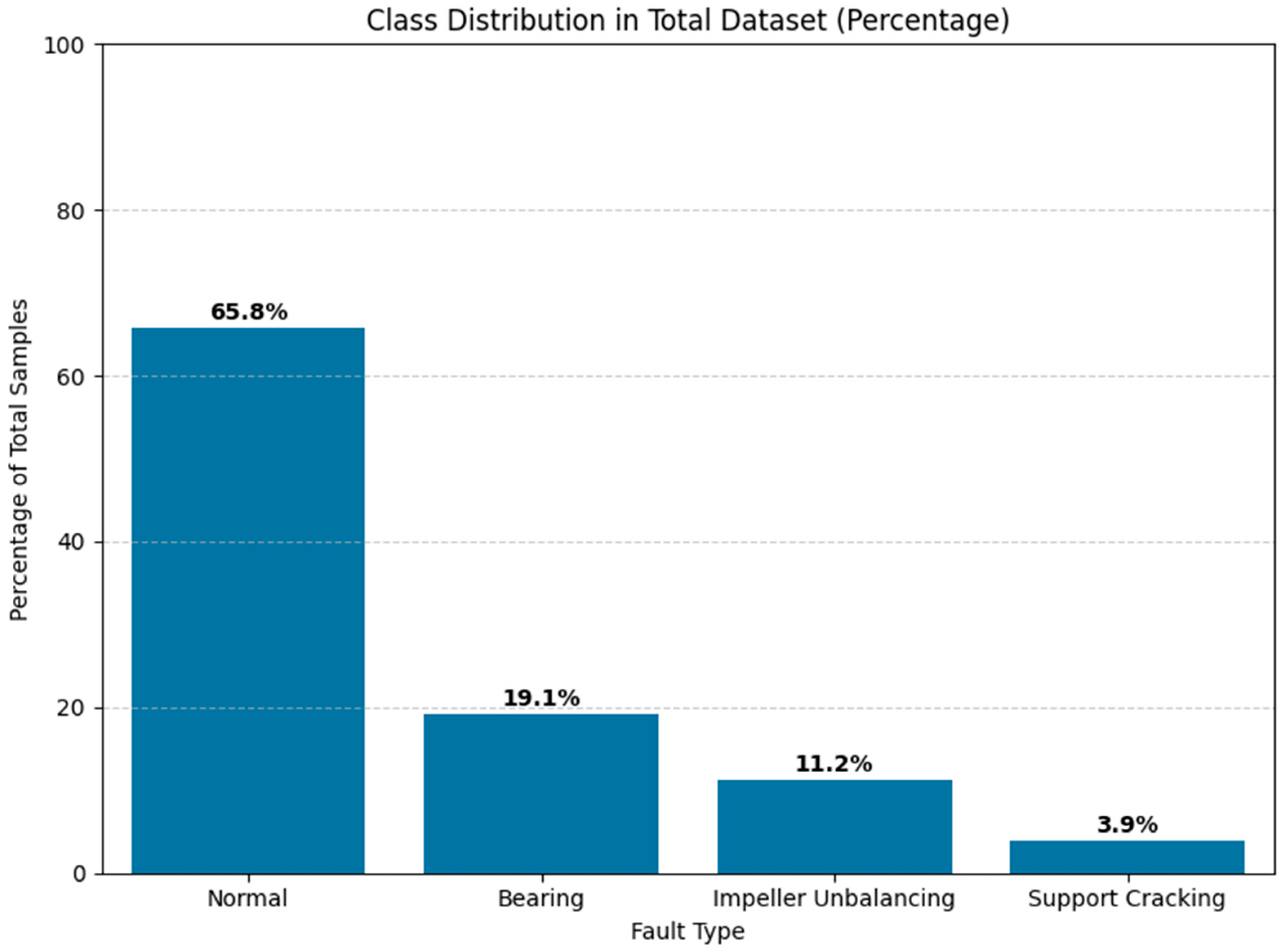
To better understand the composition of the dataset used in model training, we present the class distribution of all labeled samples collected. This distribution reflects the natural imbalance among fault types and normal conditions as captured under real production settings. Due to the rarity of some fault events and the variable duration of normal operations between stoppages, the dataset inherently contains a greater proportion of “Normal” data (
Figure 12).
In the context of our industrial air-cooling system, it was not feasible to apply traditional data balancing techniques (e.g., oversampling or undersampling) due to the inherent constraints and structure of real-world production dynamics [
25]. Fault events occur under highly specific and sporadic conditions, often driven by complex and interdependent variations in load, temperature, and motor speed. These operational states cannot be artificially reproduced on demand without interrupting production or risking equipment integrity. Moreover, altering the natural fault-to-normal ratio would require deliberately stressing machinery, introducing faults, or modifying operating parameters in ways that could compromise safety, product quality, and delivery schedules. The plant operates under strict production planning, where maintenance interventions are tightly synchronized with scheduled product changeovers, leaving no flexibility for controlled fault injection or experimental manipulation. Additionally, vibration and operational signals are continuously influenced by external factors such as fluctuating ambient temperatures, varying material properties, and downstream process loads, making it impossible to isolate and replicate specific fault scenarios without disrupting the overall manufacturing process. Consequently, the collected data inherently reflects the authentic distribution of operating states, ensuring that the diagnostic model learns from realistic temporal and operational patterns representative of actual factory conditions.
5.4. Data Availability Considerations
Obtaining large and consistently high-quality datasets remains a well-recognized challenge in industrial fault diagnosis, as real-world signals are often noisy, imbalanced, and constrained by production and maintenance schedules. In the present work, this issue is addressed by grounding the dataset in authentic operational data directly cross-validated with maintenance logs, thereby ensuring that the collected samples, while limited in number compared to laboratory studies, accurately reflect actual fault conditions and operating states. Furthermore, continuous monitoring in industrial environments naturally yields abundant sensor streams over time, progressively enhancing both data quantity (through long-term monitoring) and reliability (through systemic alignment with maintenance events). Consequently, the proposed methodology is not dependent on artificially curated datasets but is inherently designed to operate under realistic industrial data conditions, where long-term monitoring strengthens generalization and deployment feasibility.
6. Fault Classification Results
In this section, the classification results from the application of various machine learning and deep learning techniques for fault detection on our labeled data frame are presented. Different classification approaches are introduced, starting with a traditional machine learning model as a baseline before progressing to the more advanced DL architectures. Each model is trained using vibration and motor parameters collected and labeled from real production and maintenance data, aiming to accurately distinguish between normal operation and three distinct fault types: impeller unbalancing, bearing failure, and motor support cracking. In what follows, results are presented regarding the structure and evaluation metrics of each model, including accuracy, precision, recall, and F1-score, to assess their classification effectiveness. Additionally, confusion matrices and training evolution graphs provide deeper insight into each model’s performance, highlighting how well each approach generalizes to unseen data. This comparative analysis aims to determine the most suitable model for real-time fault diagnosis, ensuring early fault detection and minimization of unexpected machine failures.
6.1. Models’ Setup
Regarding the training and testing split, all models were trained on 80% of the data and tested on the remaining 20%.
Next, all DL models used the Adam optimizer (learning rate of 1 × 10⁻⁴), the categorical cross-entropy loss function, a 32 batch size, and the Softmax activation function at the output layer, and were trained for 100 epochs.
Finally, fixed time-step window sizes were utilized in all the DL architectures. The selection of step sizes was guided by an iterative empirical process aimed at balancing temporal context capture and computational efficiency across all tested architectures. For sequential models, LSTM, BiLSTM and BiLSTM + Attention, up to a 10-time-step window was found to provide sufficient historical information for sequence learning without introducing unnecessary noise or inflating model complexity. In contrast, the CNN-1D and ResNet50-1D architectures, which benefit from deeper feature extraction and residual connections, achieved optimal performance with a longer 50-time-step input, enabling it to learn richer temporal patterns while maintaining stable convergence. These choices were derived through comparative trial-and-error experiments, where multiple window sizes were evaluated for their effect on classification accuracy, training stability, and inference time. The rest of the configuration details for all six models are included in
Table 7.
6.2. Confusion Matrices and Evaluation Metrics
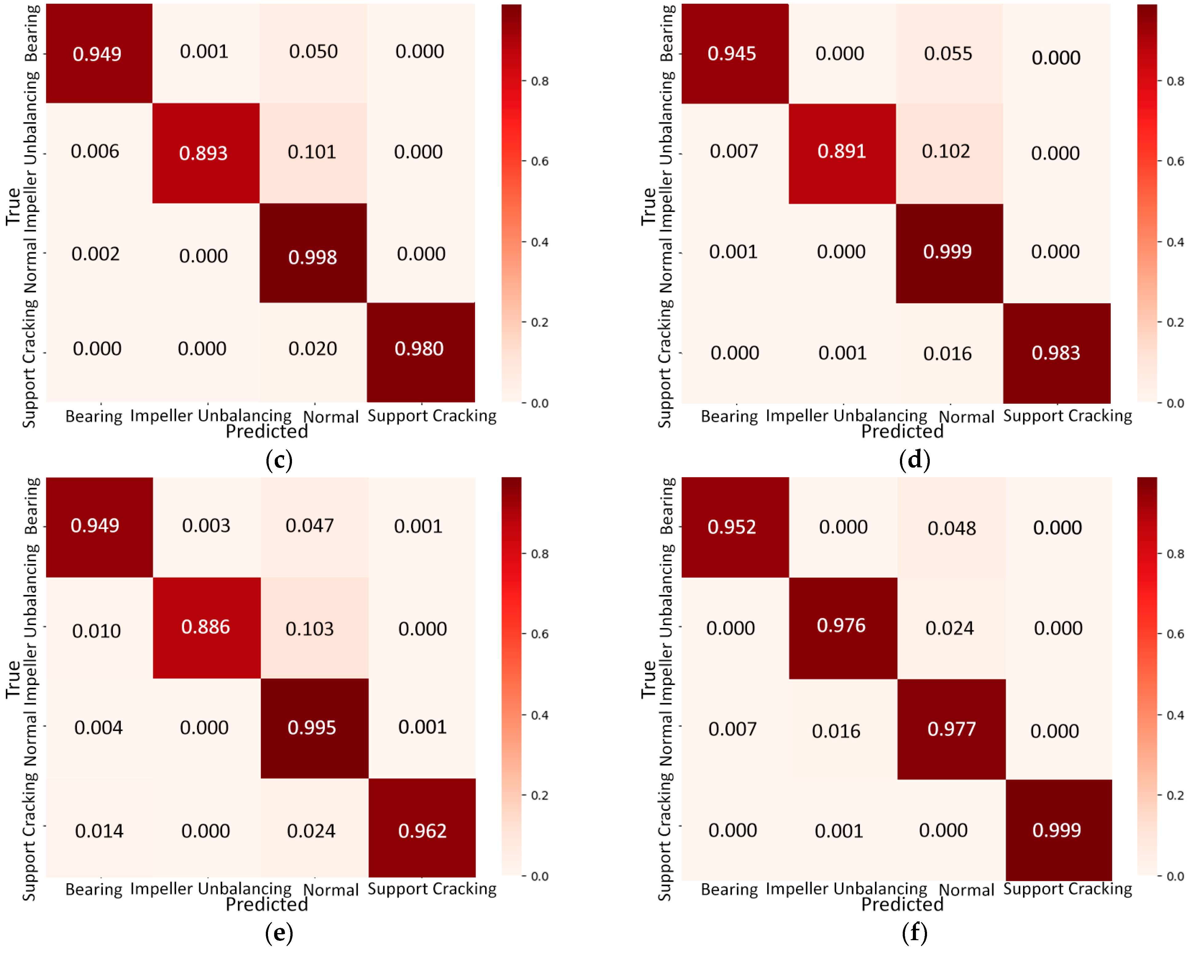
Figure 13 includes indicative confusion matrices for all models, while
Table 8 summarizes the measured performance metrics for all classification models.
Figure 13a, regarding the RF classifier, the confusion matrix demonstrates high accuracy in fault classification, particularly excelling in detecting Support Cracking (98.8%) and Bearing Faults (94.4%), indicating strong feature separability. The Normal condition is correctly classified 97.1% of the time, though 5.5% of Bearing Fault cases and 10% of Impeller Unbalancing cases are misclassified as Normal, suggesting that early-stage faults may resemble baseline vibrations. Impeller Unbalancing detection shows the highest misclassification rate (10% misclassified as Normal), highlighting the need for refined feature extraction to better distinguish its vibration patterns. While the model performs well overall, further optimization is necessary to improve early fault detection and reduce misclassification, especially in the Impeller Unbalancing fault class.
The LSTM confusion matrix (
Figure 13b) shows that the LSTM model performs well in classifying faults, with high accuracy across all categories. Normal (99.5%) and Support Cracking (95.5%) have the highest correct classification rates, while Bearing Fault (93.3%) also achieves strong but lower performance. However, similarly to the RF classifier, it also struggles to classify the Impeller Unbalancing as 10.3% of the unbalanced impeller data were misclassified as Normal, indicating that its features on this fault keep overlapping with normal conditions. In addition, it shows higher difficulty than the RF model to classify the Bearing from the Normal labels.
The confusion matrix in
Figure 13c indicates that the BiLSTM classifier slightly outperforms LSTM, with less misclassification in detecting Bearing Faults (94.9% vs. 93.3%) and better classification of Support Cracking (98.0% vs. 95.5%), reducing false positives. However, Impeller Unbalancing remains a challenge at 10.1% misclassified as Normal, similar to LSTM however, the bearing fault shows less overlapping probability than the LSTM.
Regarding BiLSTM with attention mechanism, a close look at the confusion matrix (
Figure 13d) shows only marginal improvements over the standard BiLSTM. Bearing Fault detection (94.5%) is nearly the same as in BiLSTM (94.9%), and Support Cracking (98.3%) remains strong with minimal misclassifications. Normal state accuracy (99.9%) is slightly improved, but Impeller Unbalancing misclassification (10.2%) remains an issue, similar to BiLSTM (10.1%). Despite the theoretical advantage of Attention in focusing on key time steps, its impact on performance here is minimal. While the model maintains high accuracy and stability, it does not show a significant classification improvement over BiLSTM, suggesting that the added complexity of the Attention mechanism may not be necessary for this dataset.
The CNN-1D model’s confusion matrix (
Figure 13e) reveals a slightly better classification ability than the vanilla LSTM across all the fault labels, but it is worse than the BiLSTM variations. Also, the same main misclassification issue remains with the addition of Bearing and Impeller faults overlap.
The ResNet50-1D Confusion Matrix (
Figure 13f) reveals that the model seems to finally resolve the persistent misclassification issue of Impeller Unbalancing, achieving 97.7% classification accuracy in this category, a great improvement in comparison with all the five previous models which struggled to differentiate Impeller Unbalancing from Normal states, often leading to false predictions with a classification accuracy consistently below 90%. It appears that ResNet50-1D’s deeper architecture and residual connections allow it to better capture subtle feature differences, significantly reducing these misclassifications.
As shown in
Table 8, the RF model achieves 95.80% accuracy, demonstrating strong overall classification performance. High precision (95.47%) indicates minimal false positives, while recall (94.98%) shows effective fault detection, though some cases are missing. The F1-score (95.22%) confirms a balanced trade-off between precision and recall. Despite strong results, misclassifications in Impeller Unbalancing suggest feature overlaps, highlighting the need for improvements either in feature selection or due to the struggles of this model with time-dependent fault patterns—by using time-series modeling techniques to take advantage of the time-dependent nature of our vibration-based features.
The metrics in
Table 8 indicate that the vanilla LSTM model slightly outperforms Random Forest with a higher accuracy (96.84%) and precision (97.23%), indicating fewer false positives. However, recall (94.05%) is slightly lower than desired and similar to Random Forest (94.98%), meaning some faults are still misclassified. The F1-score (95.57%) shows a similar balanced trade-off between precision and recall compared to Random Forest (95.22%). Finally, the Loss (12.57) is alarmingly high, indicating a significant difficulty in the LSTM diagnostic capability, especially on the early-stage faults.
Regarding the BiLSTM model,
Table 8 reports that it achieves a higher accuracy (97.76%) with a low loss (6.01), indicating strong learning and generalization. Its precision (98.84%) reflects minimal false positives, while the recall (95.48%) shows effective fault detection but with some missed cases, particularly in Impeller Unbalancing misclassifications. The F1-score (97.07%) confirms a well-balanced trade-off between precision and recall. Even though BiLSTM does not manage to solve the Impeller misclassification compared to the previous models, the BiLSTM manages to improve significantly the overall fault classification in all labels, making it a more reliable option so far.
The performance metrics of BiLSTM with an attention mechanism confirm the suspicion that compared to the previous BiLSTM, the improvements are minimal, indicating that the added complexity of the Attention mechanism does not significantly enhance either the overall classification performance or the permanent Impeller Unbalancing misclassification.
The vanilla CNN model achieves high accuracy (97.30%), with a slightly higher loss (8.44) compared to BiLSTM, indicating effective but slightly less optimized convergence. The precision (98.06%) remains strong, minimizing false positives, while the recall (94.82%) is slightly lower than BiLSTM, meaning some faults are still missing. The F1-score (96.35%) confirms a well-balanced trade-off between precision and recall. While CNN performs competitively, it does not significantly outperform BiLSTM in Accuracy but offers a more computationally efficient alternative.
The ResNet50-1D model achieves the highest overall classification accuracy (97.77%) with the lowest loss (3.68) among all tested models, indicating strong learning efficiency and better optimization. The precision (97.54%) and recall (97.78%) are well-balanced, showing that the model minimizes false positives while effectively detecting all fault cases. The F1-score (97.63%) confirms its consistent and reliable classification performance. Notably, this model finally resolves the Impeller Unbalancing misclassification issue, outperforming previous models. While the model still exhibits some validation instability, its ability to accurately classify all fault types, including Impeller Unbalancing, makes it the most effective candidate so far.
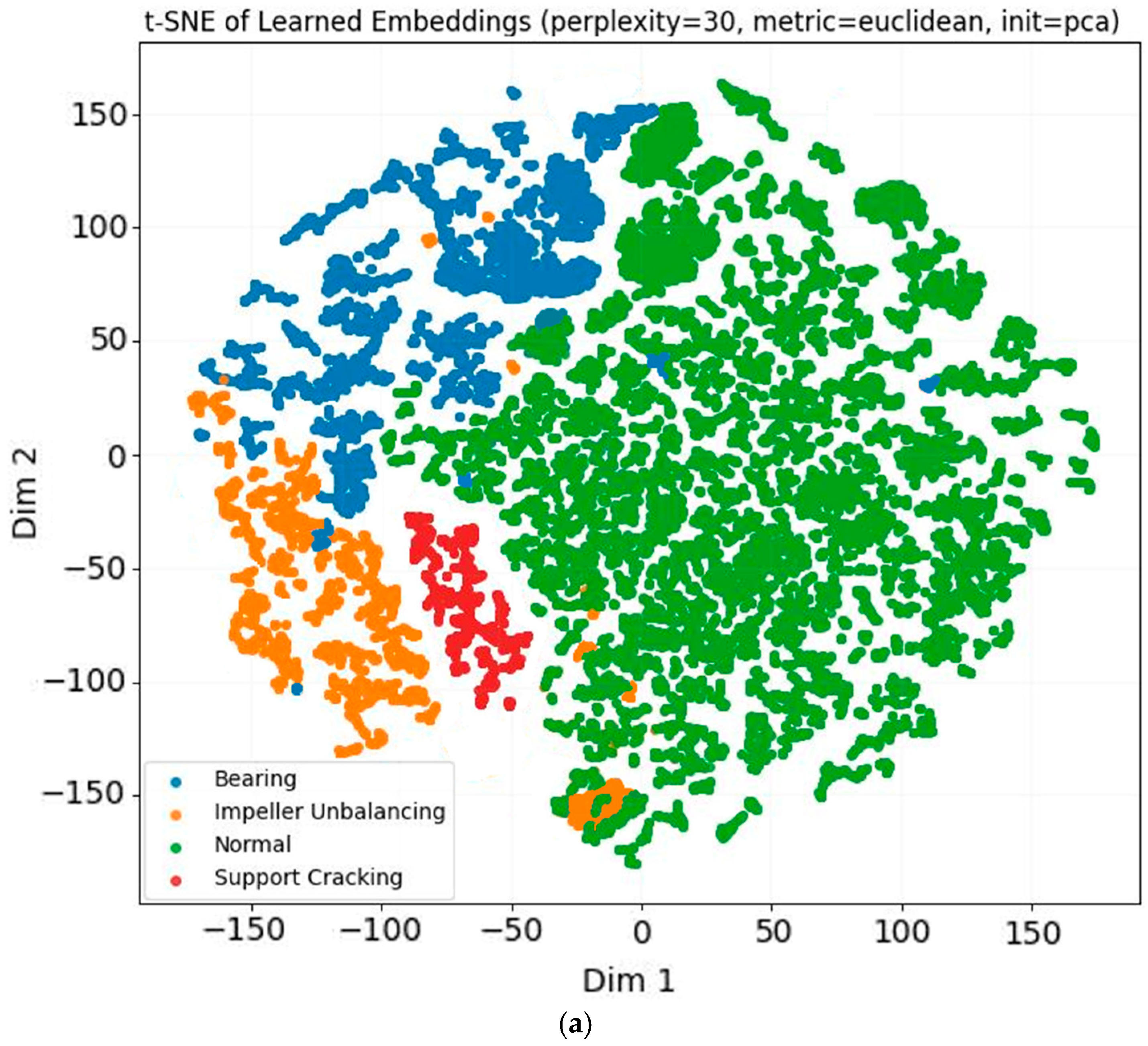
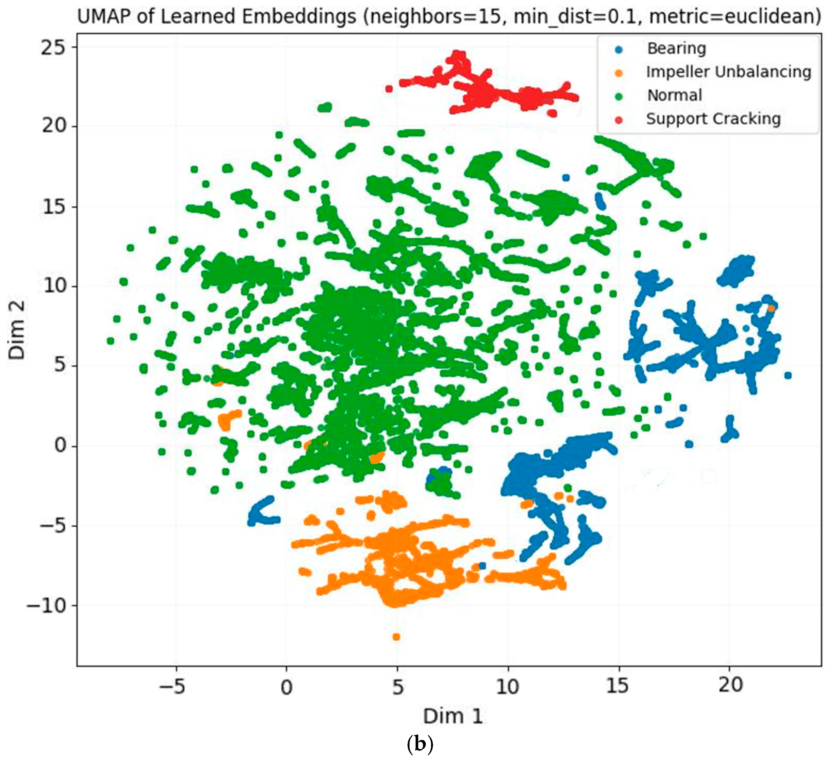
Finally, it is noteworthy that the Support Cracking class, despite representing the smallest proportion of total samples, was classified with higher accuracy than the Normal class, which accounts for the majority of the dataset. This seemingly counterintuitive result can be explained by the nature of the vibration signatures. Support Cracking produces highly distinctive patterns that diverge strongly from baseline behavior, yielding clearer class boundaries in the learned feature space. In contrast, the Normal class aggregates data collected under a wide variety of operating conditions (e.g., different speeds, loads, and ambient influences), which increases intra-class variability and partially overlaps with early fault signatures. As a result, Normal samples are more difficult to consistently classify, whereas the sharp discriminative characteristics of Support Cracking enable higher recognition accuracy despite their lower frequency. This observation is further corroborated by the visualization of the learned feature embeddings from the ResNet50-1D model. As shown in
Figure 14a, t-Distributed Stochastic Neighbour Embedding (t-SNE) projection demonstrates that Support Cracking samples (red dots) form a compact, well-separated cluster, clearly detached from the regions of the other classes. A complementary Uniform Manifold Approximation and Projection (UMAP) visualization, illustrated in
Figure 14b, exhibits a consistent pattern, reinforcing the distinctiveness of this minority class within the feature space.
6.3. Training and Validation Loss Evolution
To assess the learning performance and robustness of the deep learning models, training and validation loss curves were analyzed over 100 epochs (
Figure 14). All models demonstrated consistent convergence, with decreasing loss values across training. The LSTM model (
Figure 15a) stabilized around a higher validation loss of ~0.15, suggesting limited optimization.
In contrast, BiLSTM (
Figure 15b) achieved better convergence, with validation loss reducing to ~0.05, indicating improved learning capacity. The addition of an attention mechanism to BiLSTM (
Figure 15c) slightly improved loss stability, converging to ~0.045, though the performance gain was marginal. The vanilla CNN-1D model (
Figure 15d) maintained a validation loss of ~0.08, showing good generalization but not outperforming recurrent architecture. Finally, ResNet50-1D (
Figure 15e) achieved the lowest validation loss of just ~0.036, with minimal fluctuation throughout the training process. This demonstrates not only superior learning efficiency but also excellent consistency between training and validation loss curves, confirming its strong generalization ability and robustness under real production data variability.
For the remaining models, however, a different trend was observed, where validation loss occasionally appeared lower than training loss. Dropout regularization and batch normalization, which were applied in the recurrent and CNN-based models, introduce additional noise during training but are disabled or averaged out during validation, leading to higher training loss relative to validation loss. Moreover, the validation subset in our setup was class-balanced by design (via stratified splitting), while the training data preserved the natural imbalance of the production dataset. This difference resulted in smoother convergence on the validation set, particularly for minority fault classes that were underrepresented in training. In addition, because early stopping was not applied, transient fluctuations in training loss were more pronounced, whereas the validation curves reflected more stable generalization. Collectively, these factors explain why most models displayed lower validation loss than training loss, without indicating data leakage or overfitting, and this effect was less prominent in ResNet50-1D due to its deeper residual architecture and longer time-window training, which stabilized optimization.
6.4. Testing ResNet50-1D on Ventilator 3 Run
To evaluate the real-world diagnostic capability of the best-performing model, ResNet50-1D, we applied it to an unseen production run of Ventilator 3 that led to a bearing fault.
Figure 16 illustrates a scatterplot of the aRMS evolution along the timeline of this production run, overlaid with the predicted fault classifications.
The ResNet50-1D scatter plot demonstrates the model’s high diagnostic reliability. During the initial period, aRMS values remain stable and are correctly classified as Normal (green). As the vibration intensity increases approaching mid-April, the model progressively identifies the emergence of a Bearing Fault (red), culminating in accurate and timely fault recognition just before the scheduled stoppage. Importantly, the model avoids unnecessary false alarms, showing no erratic predictions of unrelated fault types. This clear and structured classification reinforces ResNet50-1D’s ability to detect fault evolution with precision under real production conditions, making it highly suitable for diagnostic classification in industrial environments.
6.5. Cross-Validation Evaluation
A single train/test split, although common in ML and DL benchmarks, may not provide reliable insights in the context of industrial fault diagnosis [
43]. Real-world machinery datasets are often limited in size and fault diversity, while different machines can exhibit varying operating conditions and noise patterns [
44]. As a result, models may overfit to the specific idiosyncrasies of individual ventilators, leading to optimistic but misleading accuracy values. To address this concern, we employed a combination of two cross-validation tests, which enable more stringent evaluation of model generalization [
45]. In particular, we applied a Leave-One-Vent-Out Cross-Validation (LOVO CV) to capture cross-ventilator generalization [
46,
47], and a Hybrid-Leave-One-Vent-Out combined with a 5-Fold Cross-Validation test on Ventilator 5 (LOVO + 5 Fold CV) to assess temporal robustness for rare faults [
48,
49]. Together, the two cross-validation schemes capture distinct aspects of generalization: LOVO CV tests cross-ventilator transferability for common faults, while Hybrid-LOVO + 5 Fold probes the temporal stability of models when faced with a fault observed on a single machine.
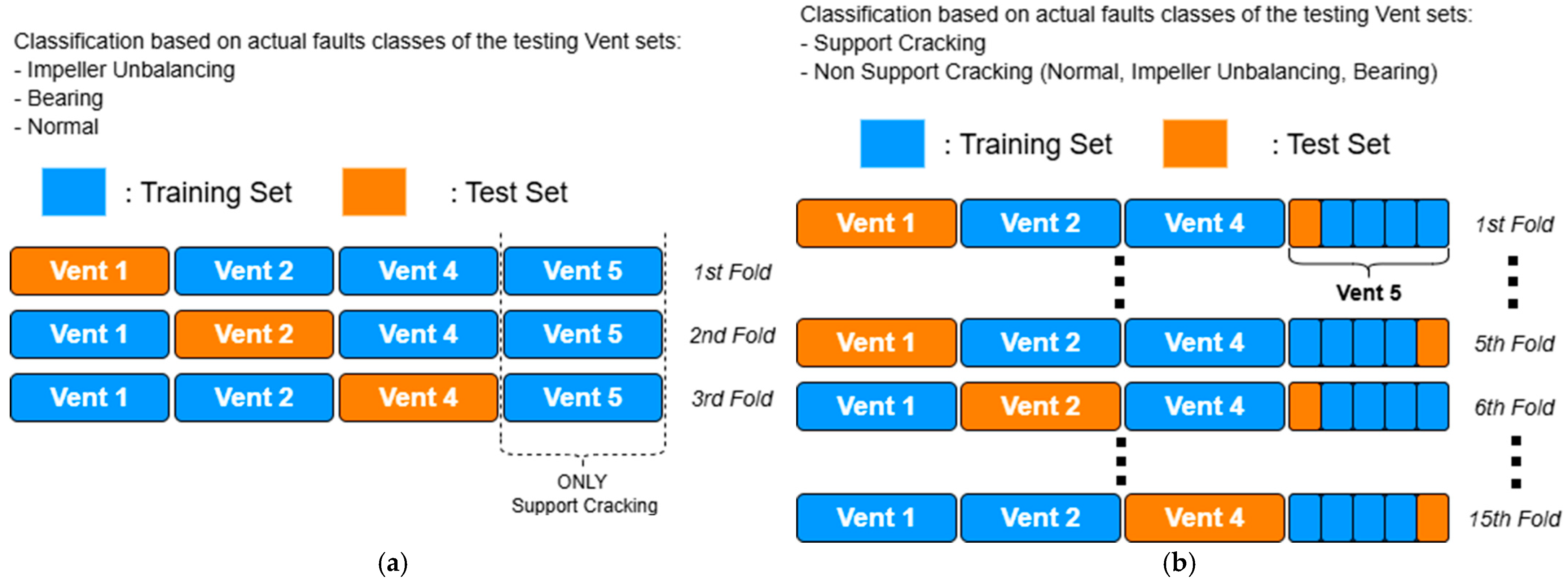
In the LOVO CV setup, each ventilator was left out in turn and used exclusively for testing, while the models were trained on the remaining ventilators (
Figure 16). This protocol evaluates whether a model can recognize fault signatures in an unseen machine, thereby assessing its ability to generalize across equipment. Bearing and Impeller faults were included in this procedure, as they appear in multiple ventilators. By contrast, Ventilator-5 was not used in the LOVO loop, since it only contains Support Cracking data and no Normal or other fault classes, making a balanced comparison infeasible.
For the Support Cracking fault, however, standard LOVO was not feasible, since this condition was only observed in Ventilator 5. Since the Support Cracking fault occurred exclusively on Ventilator 5, a standard LOVO split could not be applied. To address this limitation, we introduced a Hybrid-LOVO + 5 Fold protocol, where early Support samples from Ventilator 5 were combined with Non-Support data from other ventilators for training, and later Ventilator 5 segments were reserved for testing. This complementary evaluation provides insight into temporal robustness under rare-fault conditions rather than representing a direct improvement over LOVO. Training was performed on early Support Cracking samples together with Non-Support Cracking data (Normal, Bearing, Impeller) from the other ventilators, and testing was carried out on the later Support folds and unseen negatives (
Figure 17). This complementary test should reduce temporal leakage and provide a more realistic evaluation for this rare fault under the given data constraints [
49].
Table 9 summarizes the cross-validation outcomes for all models under both LOVO and Hybrid-LOVO + 5 Fold setups. The results from standard LOVO CV demonstrate that all models achieve balanced performance across ventilators, with ResNet50-1D showing the strongest overall generalization (Accuracy 90.8%, F1 88.6%). CNN-1D, BiLSTM, and 2BiLSTM + Attention followed closely, while Random Forest and vanilla LSTM yielded slightly lower stability. These findings confirm that deep models, particularly residual architectures, are more robust to cross-machine variations. In addition, under the LOVO + 5 folds setup, all models achieved high accuracy (97–98%), though differences in recall (e.g., Random Forest: 79.4% vs. ResNet50-1D: 87.9%) highlight their varying ability to detect minority fault signatures.
6.6. Precision–Recall Curves Evaluation by Fault Class
In this section, we assess the class-wise detection performance of each model using Precision–Recall (PR) curves. For each fault class (Support Cracking, Impeller Unbalancing, Bearing) we present PR overlays across the evaluated architectures (ResNet1D, CNN1D, LSTM, BiLSTM, BiLSTM + Attention, Random Forest) under the two cross-validation tests (LOVO and Hybrid L2VO); the curves are drawn from pooled test predictions across folds—stabilizing variance and reflecting deployment-like distributions. Curves that lie higher and farther to the right indicate better ranking of positives at a given recall; no decision threshold is fixed in these plots. For reference, the horizontal no-skill line equals the class prevalence. Below on
Figure 18, we present the three overlayed PR curves for the six models—one for each fault class (Impeller Unbalancing, Support Cracking, Bearing)—to visualize and compare model behavior at all operating points.
Across the three fault classes, the PR curves reveal distinct separability profiles. For Impeller Unbalancing, the ResNet50_1D traces the upper envelope over nearly the entire recall axis, retaining markedly higher precision through the mid–high recall band (~0.6–0.9) where CNN-, LSTM-/BiLSTM-based, and RF models begin to soften; this yields the strongest average precision and a wider operating region in which recall can be increased with only a modest precision penalty. In the Bearing class, curves from all architectures cluster tightly near the top and diverge only as recall approaches 1, indicating that errors are concentrated in a small low-signal tail—likely very early-onset cases—while the bulk of positives are ranked cleanly and similarly across models.
Finally, the PR curves for Support Cracking indicate that all models maintain consistently high precision across most recall levels, explaining the near-perfect accuracies observed under the Hybrid-LOVO setup. However, the curves diverge in the high-recall region: Random Forest exhibits an earlier decline in precision, which corresponds to its lower recall (79.4%). By contrast, ResNet50-1D and BiLSTM + Attention tend to preserve the highest precision in the extremely high-recall tail, enabling ≥ 0.9 recall with only modest precision losses. This behavior aligns with the reported recall differences (e.g., ResNet50-1D 87.9% vs. Random Forest 79.4%) and highlights that, while all models are capable of detecting the more unique but rare fault with high overall reliability, their ability to capture the complete set of positive samples varies significantly.
6.7. Computational Efficiency Evaluation
Computational efficiency is a first-order design constraint for production fault-detection systems, alongside statistical generalization. To enable fair, hardware-aware comparison across model families, we report a compact suite of cost indicators commonly adopted in modern ML systems evaluation. We quantify model capacity and memory footprint via trainable parameters and on-disk Model Size—standard proxies in contemporary compression/acceleration work that correlate with memory traffic and update cost [
50] and make storage/deployment implications explicit. We also estimate architecture-level compute with MACs/FLOPs per sample, a hardware-agnostic measure of arithmetic intensity widely used in efficient deep learning and accelerator literature [
51,
52]; nevertheless, FLOPs do not uniquely determine latency on real hardware, motivating additional wall-clock measurements [
53]. In addition, we report Training Cost as average Epoch Time and Total Training Time, which matter for iterative re-training, continuous deployment, and energy footprint—now a core topic in efficiency research [
54]. Inference serving is characterized along two complementary axes: Latency (median and p95 to capture the tail relevant to SLAs/SLOs in latency-critical services [
55]) and Throughput (samples/s or windows/s) following established benchmarking practice (e.g., MLPerf Inference single-stream/server/offline scenarios [
56]). Since algorithmic compute (FLOPs) and realized latency can diverge across devices and kernels, we complement FLOPs with hardware-aware latency measurements and tail-sensitive summaries. Together, these metrics provide a balanced view—capacity/footprint (parameters, model size), algorithmic compute (MACs/FLOPs), training amortization (epoch/total time), and serving behavior (median/p95 latency and throughput)—enabling model selection not only by accuracy but also by deployment fit (edge vs. server, real-time vs. batch), in line with current systems and benchmarking practice. Having defined the evaluation criteria, we now summarize the computational cost metrics of all candidate models in
Table 10.
From a compute–performance standpoint, ResNet50-1D is a strong default for our setting: it remains modest in size (≈254 K params; ~12.4 M MACs/window) with manageable training time (~26.9 s/epoch over 20 epochs) and real-time inference (B = 1: ~63 ms; B = 64: ~979 windows/s).
The lighter CNN-1D is far cheaper (≈50 K params; ~0.07 M MACs/sample) and trains faster (~13.7 s/epoch), with similar batched throughput (~1045 samp/s), making it attractive when frequent redeployments or on-device updates matter more than peak accuracy. Recurrent models invert this trade-off at serving time: the BiLSTM sustains extremely low latency (B = 1: ~2.1 ms; B = 64: ~33 k samp/s) despite higher training cost (~53.8 s/epoch) and a moderate footprint (~80 k params; ~0.78 M MACs/sample). Adding attention barely changes size (~80 K params) or MACs, and preserves sub-3 ms latency, while slightly increasing training time (~56.5 s/epoch); this variant is appealing when interpretability and temporal focus are useful. The plain LSTM minimizes complexity (≈13 K params; ~12.8 K MACs/sample) but trains slower per epoch (~28.8 s) and offers only modest latency gains (B = 1: ~55 ms), making it a good baseline for severely constrained devices. Finally, Random Forests fit very fast (~6.9 s) and score quickly on CPU (B = 64: ~2653 samp/s) but carry a large memory footprint (~90 MB for 100 trees) and lack temporal inductive bias. In practice: prefer ResNet50-1D when overall accuracy/robustness is paramount, CNN-1D for footprint/retraining efficiency, BiLSTM (+Attn) for ultra-low-latency streaming, and RF for simple CPU-only deployments.
6.8. Overall Evaluation
After evaluating multiple classification models, ResNet50-1D stands out as the most effective for fault detection and is deployable for maintenance frameworks. The cross-validation tests confirmed its ability to transfer across machines and remain stable under rare-fault conditions, while class-wise PR curves showed its advantage in maintaining precision at high recall levels compared to simpler models. At the same time, both the initial train test confusion matrix and the latter class-wise PR curve show that it resolves the persistent misclassification of the impeller unbalancing fault, demonstrating strong generalization and enhanced feature extraction capabilities.
However, ResNet50-1D is not without limitations. Fluctuations in validation curves indicate some sensitivity to data variability, and its deeper architecture requires higher computational resources, which may limit use in low-power real-time settings. Computational efficiency analysis highlighted useful alternatives: CNN-1D as a lightweight option for frequent redeployment, BiLSTM variants for ultra-low-latency scenarios, and Random Forest for simple CPU-based deployments.
Overall, ResNet50-1D provides the best balance of accuracy, generalization, and deployment readiness, making it the most reliable backbone for industrial integration. Nevertheless, alternative models retain value under specific resource or latency constraints, and further tuning may help strengthen the stability of the preferred architecture in future work. A key reason for the superior performance of ResNet50-1D lies in its architectural design. Unlike shallower CNNs or recurrent models, ResNet50-1D employs residual connections that enable the training of deeper networks without gradient degradation, allowing the extraction of richer hierarchical features from the vibration and motor signals. This deeper feature representation proved particularly effective in disentangling subtle fault patterns such as Impeller Unbalancing, which were consistently misclassified by other models. In addition, the longer time-windowing strategy (50 steps) combined with residual learning enabled the model to jointly capture both temporal dynamics and spectral–spatial characteristics of the signals, achieving higher separability in the learned feature space. While Random Forest and recurrent models rely on either tabular features or sequential dependencies, ResNet50-1D integrates both local and global information, thereby offering more robust generalization under production variability.
7. Maintenance Strategy
In this section, a three-step maintenance framework is conceptualized and is tailored to the real-time maintenance needs of the company.
As a first design step, namely “Real-time Continuous Monitoring”, we need to establish a continuous feeding of the trained model with real-time data in the right format, which then enables a continuous export of labeled data on a daily basis.
We then use the best performing classifier for fault detection, i.e., the Resnet-50 classifier, to establish a detection likelihood for each fault. This leads to the second step of the framework design, namely “Fault Risk Assessment”, which is to decide on the maintenance action steps. For that purpose, we set three detection thresholds for each class. Using a modified version of the traditional Risk Assessment Matrix (RAM) methodology as a guiding tool, we then combine the detection likelihood from our classification model with the knowledge-based fault impact to decide on the fault severity level. By setting a specific set of maintenance actions for each severity level, we conclude the severity-based decision-making mechanism.
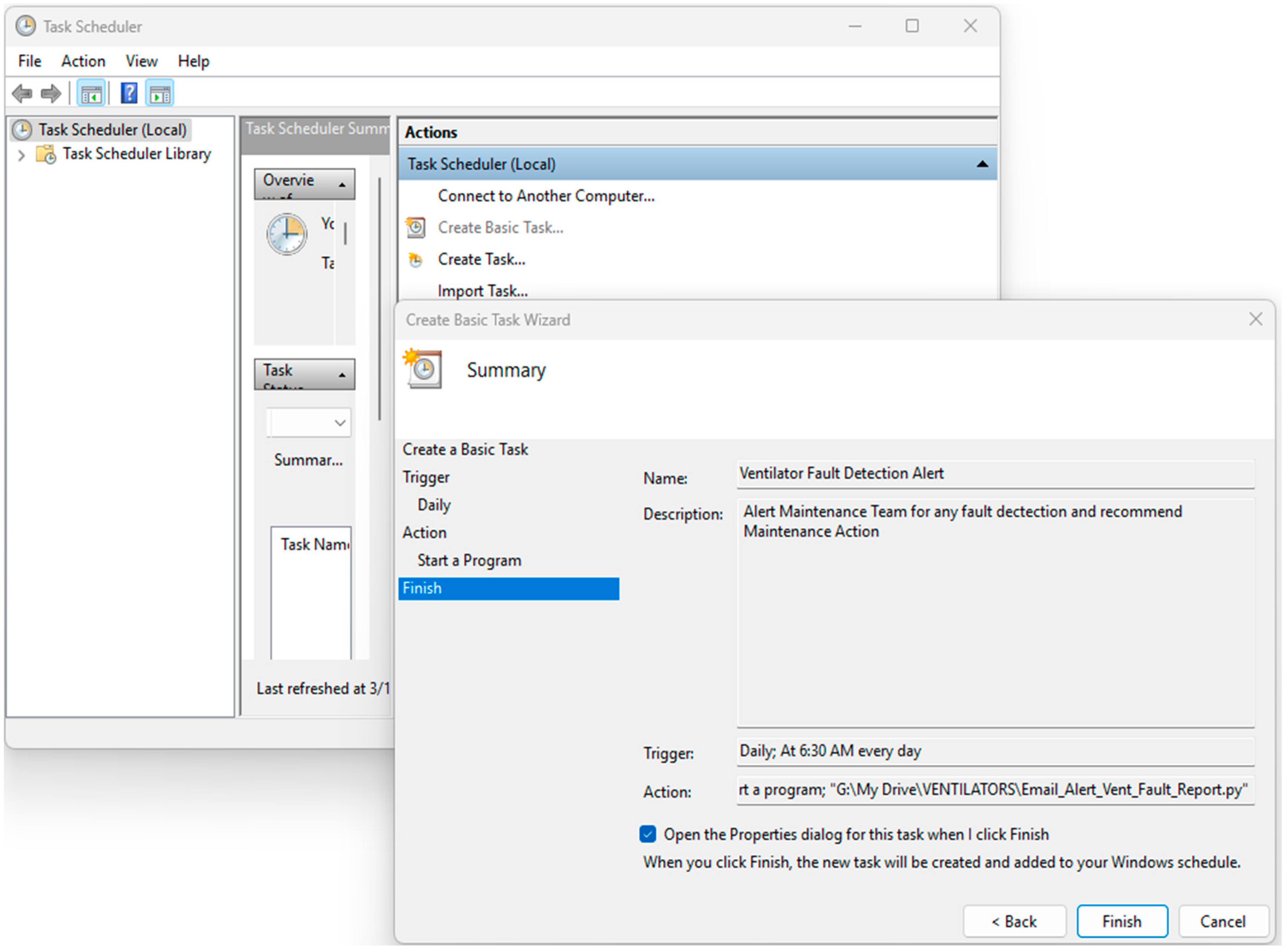
The third and final step is concluded by setting up a daily automatic notification system in case the DL classifier detects any fault and followed by recommended maintenance action, namely “Maintenance Actions”. This is established by initially setting up a simple Windows Task Manager routine combined with a Python version 3.12 script that triggers the DL classification model application. This day-to-day alert mechanism notifies every morning via email the maintenance department team in case of detecting any of the three fault categories on any of the five ventilator motors and recommends a severity-based maintenance action, respectively.
7.1. Real-Time Continuous Monitoring
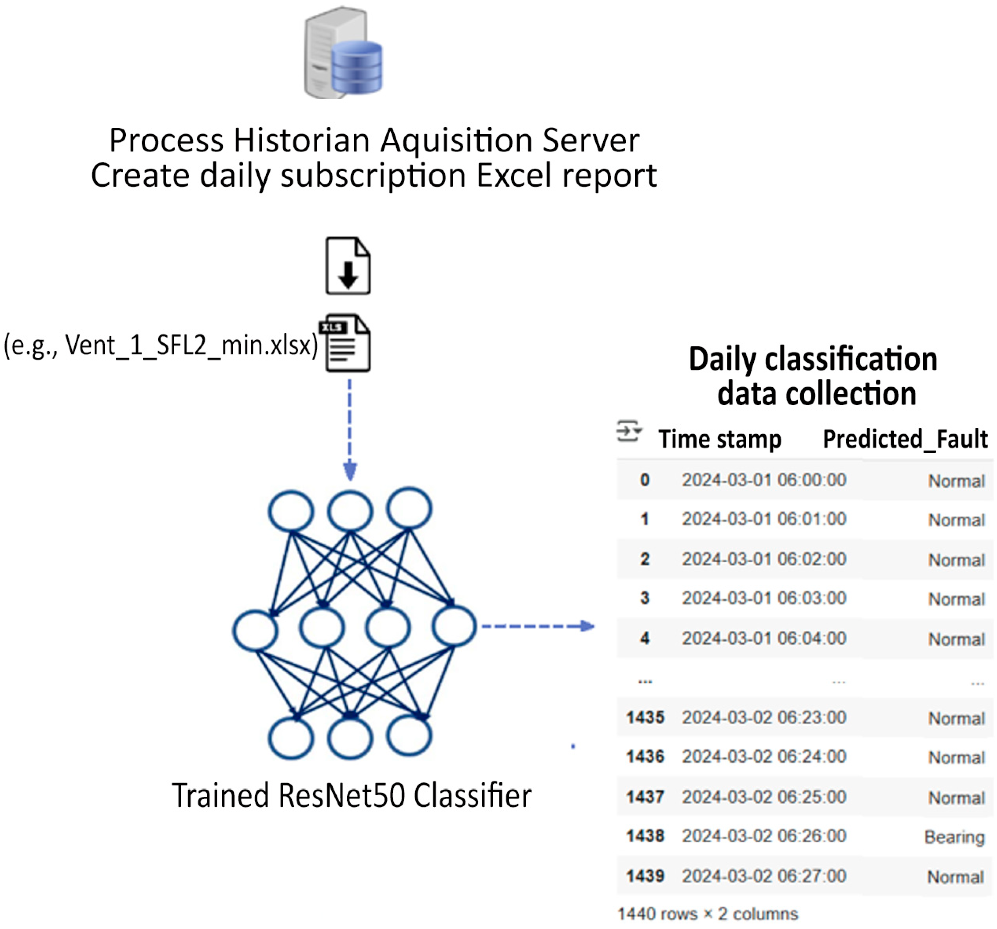
The vibration data are collected and stored on the Process Historian acquisition server, which also provides the capability to generate Excel reports, as presented in
Figure 19. This feature enables the real-time feeding of our ResNet50-1D classifier, making it possible to construct a real-time maintenance framework for early fault diagnosis.
The Process Historian feature through the Siemens interface is employed for creating a daily Excel export of all the vibration features of the four ventilator motors. This is possible by utilizing the subscription feature of the Siemens Process Historian acquisition server. At the end, a time trigger in the form of a “subscription” is created, which exports 1440 data values of all the features for the past day for each ventilator.
7.2. Fault Risk Assessment
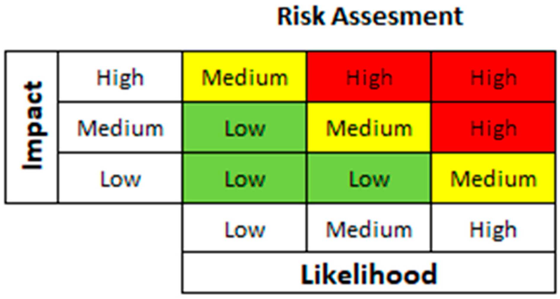
Assessing fault severity is crucial to preventing real-time unexpected failures and optimizing equipment reliability. For that purpose, we employ a traditional 3 × 3 risk assessment matrix-type approach in which each combination of fault likelihood and impact is mapped to a risk level (Low, Medium, or High), where Low risk may require routine monitoring, Medium risk calls for preventive actions, and High risk demands urgent intervention (
Figure 20) [
57]. This approach provides a simple yet effective and structured approach for prioritizing maintenance efforts by focusing on the most critical risks, ensuring more timely interventions, minimizing downtime and operational risks while maximizing asset lifespan.
After establishing this baseline, we attempt to conceptualize a modified severity-based assessment matrix by incorporating fault-specific impact and detection likelihood levels tailored to our arrangement. The resulting severity should be able to inform targeted classification-based maintenance actions, such as scheduled inspections, on-site monitoring, or immediate stoppage and replacement of critical components. For that purpose, it is necessary to properly define the fault impact and likelihood entities according to the DL classifier output.
The simple guiding principle behind the definition of fault Impact is based on:
- 1.
The specific faults’ respective mechanical consequences and failure progression within the ventilator motor system.
- 2.
The factory maintenance team accumulated knowledge and vast experience of these faults.
More specifically, for each fault, the assigned impact is provided in the following.
Support Cracking—High Impact. Support cracking directly affects the structural integrity of the ventilator motor. Cracks in the motor support can lead to severe misalignment and potential detachment of the motor from its mounting, posing an immediate safety risk. Unlike internal faults, structural failure is often abrupt, causing a complete system shutdown or even physical damage to surrounding components. The maintenance team also provided us with many historical cases of similar arrangements in which undetected cracks on the motor’s mounting caused complete and immediate failure. This justifies its classification as a high-impact fault requiring immediate stoppage and replacement.
Bearing Faults—Medium Impact. Bearing faults are progressive failures, meaning they develop over time due to wear, lubrication issues, or contamination. While degraded bearings increase friction, heat, and vibration, leading to efficiency losses and potential rotor misalignment, they do not immediately cause catastrophic failure. However, if left unaddressed, bearing degradation can escalate into severe damage to the motor shaft, overheating, or seizure, which can lead to unplanned downtime and motor burnout. Thus, bearing faults are classified as medium impact, requiring visual inspections and condition monitoring to track their progression before intervention becomes critical.
Impeller Unbalancing—Low Impact. Impeller unbalancing primarily affects rotational stability, causing excessive vibration and uneven load distribution on the motor shaft and bearings. While this does not immediately cause a failure, prolonged operation under imbalance can lead to accelerated bearing wear, increased energy consumption, and potential fatigue fractures in the motor components. The nature of impeller unbalancing allows for controlled monitoring and corrective balancing before severe damage occurs, which is why it is categorized as low impact rather than medium or high impact. In this case, the maintenance team mentioned that on multiple occasions in similar ventilation arrangements, the ventilation continued working with a slightly unbalanced impeller for several months, but at the cost of not only significant wear on the other mechanical components but also much lower cooling efficiency.
The fault impact classification reflects the risk associated with each fault type and its potential impact on ventilator motor operation. In summary, Support Cracking faults have a high impact due to their immediate and catastrophic consequences, while Bearing Faults and Impeller Unbalancing are medium and low impact, respectively, as they allow for predictive monitoring and scheduled intervention before leading to total failure. This structured classification ensures that maintenance actions are prioritized effectively to enhance system reliability and minimize downtime.
A fault detection likelihood (FL) percentage is determined by analyzing the classified proportion of predicted fault labels within the total dataset for each ventilator. After processing the daily vibration data file, the pre-trained DL model classifies each data entry into one of the predefined fault categories: Normal, Bearing Fault, Impeller Unbalancing, or Support Cracking. The script then counts the occurrences of each fault type and computes the percentage of each fault label relative to the total number of classified instances during the whole passing day using the following equation:
Next, detection likelihood thresholds are determined to support a severity-based maintenance framework, ensuring a structured and data-driven approach to fault classification. More specifically:
- 1.
FL between the [0, 25%) range represents a low likelihood, indicating that faulty occurrences are minimal compared to the total dataset. These cases suggest early-stage anomalies that do not require immediate action but should be monitored over time.
- 2.
FL between the [25, 75%) range corresponds to medium likelihood, where fault instances are more frequent and may indicate a developing issue that requires visual inspection and on-site monitoring to assess its progression.
- 3.
FL between the [75%, 100%] range corresponds to high likelihood, signaling a dominant fault presence that necessitates immediate intervention to prevent system failure.
This detection likelihood classification method ensures that maintenance actions are aligned with the severity and prevalence of faults, allowing for proactive decision-making while minimizing unnecessary interventions.
Defining the Impact and Likelihood of each fault enables us to determine each fault’s severity through the following equation:
We can now employ a modified Severity Assessment 3 × 3 Matrix to systematically evaluate the likelihood and impact of detected faults on the ventilator motors based on the DL classification data and the fault Impact guideline, as presented in
Figure 21. This matrix categorizes the ventilator faults into Low, Medium, and High Severity Levels, guiding maintenance decisions by correlating fault probability with its potential consequences on the ventilator motor. The resulting severity classification informs targeted maintenance actions, such as scheduled inspections, on-site monitoring, or immediate stoppage and replacement of critical components based on the capability of our DL classifier.
7.3. Maintenance Actions
The final part of the severity-based maintenance framework concludes by assigning specific recommended maintenance actions to each severity level. Below, we provide a summarized list of each fault:
🚨 High Fault Severity → STOP Now! Inspect and Replace!
“The structure is at risk of failure. Immediate shutdown and component replacement are necessary.”
⚠️ Medium Fault Severity → Visual Inspection and On-Site Monitoring Needed!
“Routine monitoring is required, but immediate action is not necessary unless worsening trends are observed.”
🔹 Low Fault Severity → Schedule Inspection on Heads Change-Over!
“No immediate action is required, but an inspection should be planned during the next scheduled maintenance window.”
To enhance the efficiency of our maintenance framework, an automated notification system has also been developed using a Python-based script combined with Windows Task Scheduler for scheduled execution. Here, it is important to mention that this Fiber production line works on a 4-shift base and the 1st shift starts at 6:00 AM. This means that the working day for the factory changes at 6:00 AM (not at 00:00 AM).
The Python script reads the daily vibration data report that the Process Historian provides every morning at 6:00 AM for the past working day, identifies faults by loading them on the trained ResNet50-1D classifier, and classifies their severity based on the severity assessment matrix. Following that, it extracts the ventilator number from the most current data filename, calculates fault likelihood percentages, and automatically determines the appropriate maintenance actions. Whenever the data file is not exported from the Process Historian due to any server error, the corresponding alerts of error are emailed as well to notify the team to check the system and manage the missing values.
Next, by integrating with Windows Task Scheduler, as presented in
Figure 22, the system operates autonomously, eliminating the need for manual execution and ensuring continuous fault monitoring.
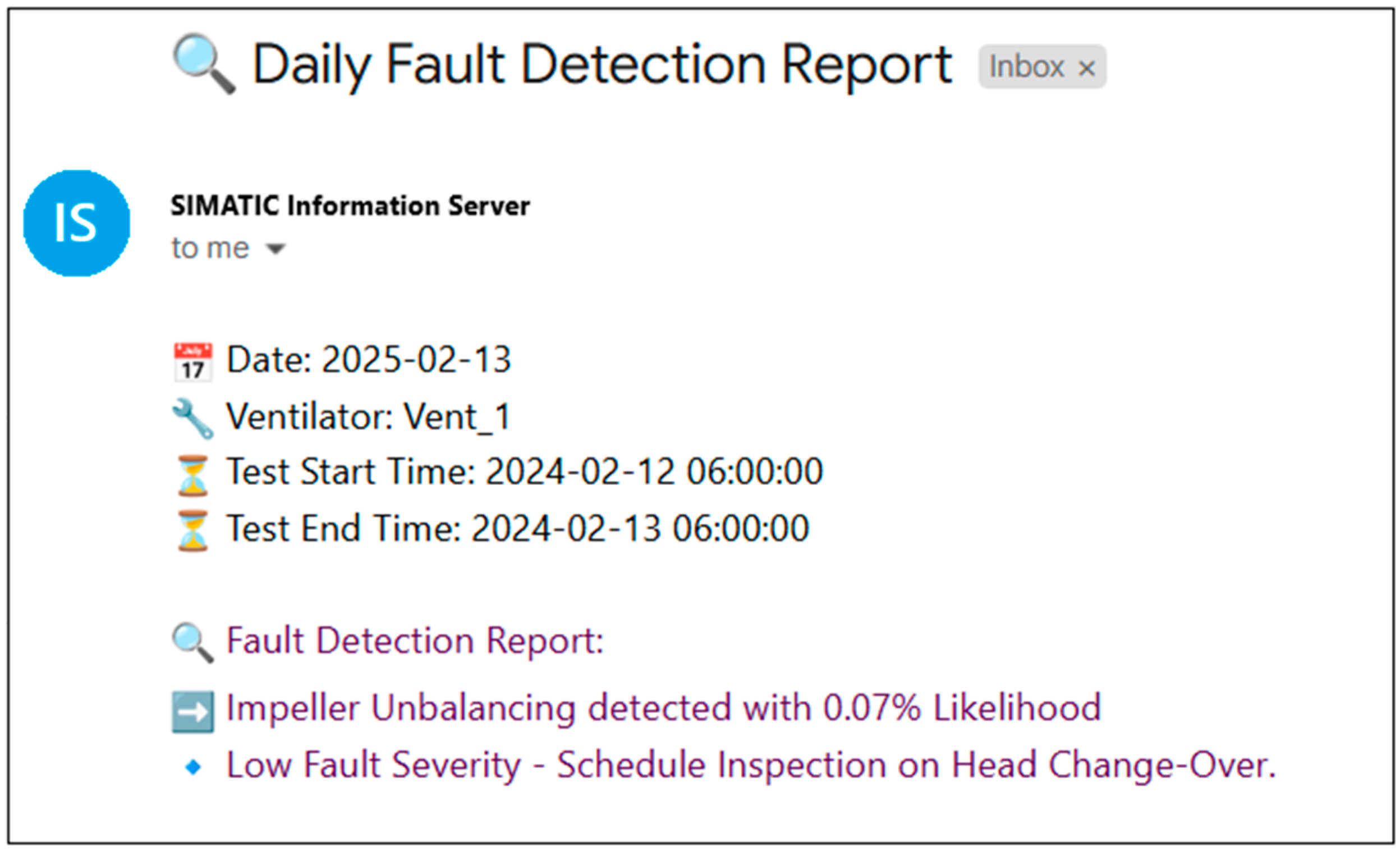
Finally, in case of any faults detected on any of the ventilator motors, the scheduled Python script generates and sends an automated email alert to the maintenance team at a fixed time each day (we set at 6:30 AM to be aligned with the maintenance team briefing), ensuring early detection and timely intervention. The email includes critical details such as the date, ventilator ID, test duration (start and end time), fault likelihood percentages, and recommended maintenance actions. As indicated in
Figure 23, on 13 February, the maintenance team was notified of a low severity of impeller unbalancing on ventilator 1, accompanied by an inspection scheduling of the Impeller on the planned preventive maintenance of the line (on the scheduled spinneret heads change-over).
At the end of February, during the planned 8-h change-over, the ventilator 1 Impeller was inspected, and no damage to the impeller was detected, only a small amount of accumulated material on the inlet duct was found. That very low severity notification was aligned with the actual inspection report of the technician. As a result, the low severity level recommended action did not waste machine availability and technical support during production, except only the planned cleaning and inspection time during the scheduled stoppage, demonstrating the robustness and cost-effectiveness of our framework.
7.4. Redundancy Considerations
In addition to continuous monitoring, risk assessment, and automated maintenance actions, industrial reliability is reinforced through redundancy mechanisms. In the studied fiber production line, hardware redundancy is already present, as multiple ventilators operate in parallel across the quenching stage. This configuration ensures that production can continue even if one ventilator requires inspection or replacement, minimizing the impact of single-unit failures.
Redundancy is also reflected at the sensing level. The diagnostic framework exploits multiple feature channels—vibration velocity and acceleration metrics (vRMS, aRMS, aPeak, Crest), together with motor temperature, current, and speed—which act as complementary indicators of machine health. This diversity of inputs enables a form of analytical redundancy, where abnormal patterns in one modality can be cross-checked against others, reducing the risk of false negatives or misleading classifications caused by a single noisy signal.
In addition to sensor- and hardware-level redundancy, the proposed framework also leverages information redundancy by aligning diagnostic labels with maintenance logged events. This systemic alignment ensures that ground truth is not inferred solely from sensor anomalies but corroborated with actual interventions, increasing the reliability of training and evaluation [
49,
58].
8. Future Work
The computational cost of deep networks, particularly for real-time applications, raises concerns about deployment feasibility in low-power industrial environments. Future work should explore model compression techniques, such as quantization or pruning, to optimize inference speed without compromising classification performance. Future work should also explore additional fault types and adapt the proposed approach to other rotating machinery with similar sensor configurations. At the level of generalization, this adaptation would involve tailoring the methodology to the operational and environmental conditions of the new setting, ensuring effective performance under different equipment designs and operating contexts.
Beyond classification, an important direction is the integration of fault severity assessment and predictive maintenance frameworks. This study proposed a severity-based decision-making approach, but further validation is needed in real-world production settings for a longer production time horizon. Incorporating explainable AI (XAI) techniques could improve interpretability, providing maintenance personnel with clear insights into why faults are detected. Moreover, expanding the dataset with diverse operational conditions and additional fault cases will enhance model robustness and adaptability.
Another important consideration for future work is model interpretability. While this study focused on achieving high classification performance, understanding why a model predicts a certain fault type is essential for trust and adoption by human maintenance teams. Techniques such as SHAP values, attention weight visualization, or other feature attribution methods could be applied to highlight the contribution of each input feature to a given prediction. This would provide maintenance personnel with transparent, explainable insights into model decisions, facilitating more informed interventions and increasing confidence in automated diagnostics. Future research would incorporate such interpretability mechanisms into the proposed framework to ensure it remains both actionable and trusted in real industrial settings.
From a practical integration perspective, the proposed system could be embedded into existing Computerized Maintenance Management Systems (CMMS) as an automated alert and decision-support tool. By continuously monitoring sensor data in real time, the model could trigger maintenance alerts when a potential fault is detected, enabling maintenance teams to schedule interventions during planned production stoppages, thus minimizing unplanned downtime. Such integration would allow the optimization of maintenance cycles, better allocation of resources, and a data-driven approach to spare parts management, ultimately improving operational reliability and reducing costs.
Finally, real-time deployment and continuous learning mechanisms should be considered, enabling the model to adapt dynamically to new operational patterns and evolving fault conditions. Implementing edge AI solutions for on-device fault classification could reduce latency and enhance industrial applicability. In addition, future work could investigate the effect of sensor fusion—combining vibration and temperature data—versus individual sensor streams, to determine whether multi-sensor integration can further improve fault detection accuracy and robustness in real-world industrial environments. A final future addition should also include the application of data augmentation through synthetic fault generation techniques to address class imbalance and the scarcity of certain fault types and investigate how this could improve the model’s generalization capability under industrial varying characteristics. By addressing these challenges and refining the framework, this work lays the foundation for a scalable, AI-driven real-time diagnostic maintenance system capable of minimizing unexpected failures and improving industrial reliability.
9. Conclusions
This industrial air-cooling study demonstrated the effectiveness of DL-based fault detection for industrial air-cooling systems, leveraging multi-sensor vibration and operational data to classify faults and support maintenance strategies. By systematically comparing multiple models—including traditional ML (RF), sequential models (LSTM, BiLSTM, BiLSTM + Attention), convolutional architectures (CNN-1D), and residual networks (ResNet50-1D)—we identified ResNet50-1D as the most reliable framework. It achieved the highest classification accuracy and lowest loss, while resolving the persistent misclassification of Impeller Unbalancing observed in other models. The model’s deeper residual architecture, in combination with longer time-windowing, enabled the extraction of richer hierarchical features, contributing to superior fault differentiation and robustness under real production variability. To strengthen this evaluation, three complementary analyses were conducted. Cross-validation demonstrated consistent generalization across different ventilators, reducing the risk of model overfitting to specific machines. Class-wise PR curves highlighted that ResNet50-1D maintained both high recall and precision, particularly in detecting Impeller Unbalancing and Bearing Faults, outperforming recurrent and CNN-based alternatives. Finally, computational efficiency analysis revealed the trade-off between accuracy and deployment cost, showing that while ResNet50-1D requires more resources than lighter models (CNN-1D, RF), its performance gains justify integration in production-critical environments. Beyond classification, the integration of diagnostic outputs with maintenance logs allowed the development of a severity-based prioritization scheme, demonstrating how DL predictions can be translated into actionable maintenance insights. Collectively, these results confirm that advanced deep learning architectures can bridge the gap between academic model development and industrial deployment, offering scalable solutions for predictive maintenance in production environments.
