Article

Fatigue Life Prediction of Main Bearings in Wind Turbines Under Random Wind Speeds

School of Mechanical Engineering, Xinjiang University, Urumqi 830046, China
*
Author to whom correspondence should be addressed.
Machines 2025, 13(10), 907; https://doi.org/10.3390/machines13100907
Submission received: 18 August 2025 / Revised: 12 September 2025 / Accepted: 29 September 2025 / Published: 2 October 2025
(This article belongs to the Section Machines Testing and Maintenance)

Abstract

To address the complex operating conditions and challenging dynamic characteristics of bearings in the main shaft transmission system of wind turbines, this study investigates a specific wind turbine model. By comprehensively considering factors such as main shaft structure, cumulative damage, and stochastic wind loads, we adopt a modular analysis framework integrating the wind field, aerodynamics, the structural response, and fatigue life prediction to establish a method for predicting the fatigue life of main shaft bearings under stochastic wind conditions. To verify this method, the fixed-end main shaft bearing of a 4.5 MW wind turbine was selected as a case study. The research results show the following: (1) Increases in both average wind speed and turbulence intensity significantly shorten the fatigue life of the bearing. (2) Higher turbulence intensity amplifies the dispersion of the speed and load of rolling elements, thereby increasing the probability of extreme operating conditions and exerting an adverse impact on fatigue life. (3) The average wind speed has a significant influence on the overall fatigue life: within a specific range, the fatigue failure probability of the main bearing increases as the average wind speed decreases. (4) The impact of wind speed fluctuations on the hub center load is much greater than that caused by rotational speed changes. (5) In addition, the modular design method adopted in this study calculates that the fatigue life of the fixed-end bearing is 28.8 years, with an overall error of only 0.8 years compared to the 29.6-year fatigue life obtained using Romax simulation software. This research provides important theoretical references and engineering value for improving the operational reliability of wind turbines and enhancing the accuracy of bearing fatigue life prediction.

1. Introduction

Wind energy constitutes one of the most rapidly growing electricity generation sources. However, turbines operating in extreme environments frequently experience premature component failures. Research demonstrates that main shaft bearings exhibit particular vulnerability to premature failure, with actual service lives consistently falling below theoretical design lifetimes [1]. This accelerated degradation occurs primarily because main bearings support substantial rotor and shaft masses while simultaneously being subjected to severe dynamic loading from stochastic environmental conditions—including variable wind fields, atmospheric pressure fluctuations, and random load variations. Consequently, accurate fatigue life analysis requires careful assessment of random wind speed effects.
Current research on the fatigue life of wind turbine main shaft bearings primarily focuses on three directions: multiphysics coupling modeling, dynamic load characteristic analysis, and data-driven life prediction methods. Additionally, advanced techniques such as stochastic resonance array technology and noise-enhanced weak signal detection in fractional-order nonlinear systems demonstrate significant potential for extracting subtle fault features in high-noise environments, offering new perspectives for condition monitoring and fault diagnosis [2,3,4]. (1) In the field of multi-field coupled modeling, Li et al. [5] combined the thermal-fluid-solid coupling model with Voronoi microscopic characterization to analyze the bearing microscopic stress and motion law, and established the fatigue life prediction method. Lu et al. [6] proposed the CDTA method (coupled diffusion process + time-attention mechanism), which can significantly improve the accuracy of residual life prediction through the enhancement of time-sequence features (PHM 2012 dataset). Zhao et al. [7] combined the multi-axis load statistics and transient contact model to predict the wheel bearing life through the improved LP theory and iterative algorithm, and the validity was verified by a bench test. (2) In the field of dynamic load characterization, Wang et al. [8] improved the LP theory to establish a damage model considering the load sequence, revealed the influence of variables through sensitivity analysis, and verified the validity of the model with 6209 bearings; Cavacece et al. [9] revealed the interfacial degradation mechanism of self-aligning roller bearings under high load oscillations through durability testing and topographic analysis, and compared it with deep groove ball bearings. Kong et al. [10] developed a dynamic model of a gear-bearing system, revealing that the load fluctuation caused by meshing significantly reduces the life, and corrected the prediction deviation of the static model. William Jacobs et al. [11] explored the dynamic change in the oil film and the early polished wear (0.5% of the life period) under high variable loads through multi-axis acceleration tests, revealing the early failure mechanism. Guo et al. [12] combined vehicle–rail dynamics and LP theory to propose a life prediction method for motor bearings considering wheel–rail impacts, revealing the accelerated damage effect of flat scars >30 mm. (3) In the data-driven field, Gao et al. [13] constructed a degradation model based on Bayesian theory, fused the vibration features and dynamically updated the parameters by the M-H algorithm to achieve accurate life prediction in the XJTU-SY dataset. Ying et al. [14] established a 4-stage model with roughness/cracking, dynamically updated the parameters by RMS, and realized the crack growth as an indicator of free crack growth. Guo et al. [15] fused the gray model/CEEMD/RVM and realized long-term stable prediction by error reconstruction and online update.
However, studies specifically addressing the fatigue life of main bearings under the direct influence of random wind speeds remain scarce. This gap stems from two main challenges: the strong spatiotemporal randomness of wind fields leading to complex, fluctuating bearing loads, and the high cost and difficulty in obtaining the massive real-world data required for traditional data-driven methods.
To address these challenges, this study proposes a novel modular framework for predicting main bearing fatigue life under random wind conditions. The main contents of this study are as follows: (1) A turbulent wind speed model is established by superimposing sinusoidal waves of specific frequencies and modes, and a time-varying wind field with different mean wind speeds and turbulence levels is obtained according to the design standard of the International Electrotechnical Commission (IEC). (2) Based on the BEM theory, the aerodynamic loads of wind turbine blades are calculated, and the transformation from random wind speed to hub center load is realized. (3) Taking the main shaft structure of a 4.5 MW wind turbine as the object of analysis, the internal and external loads of the wind turbine are converted into axial and radial loads applied to the fixed-end main shaft bearing through mechanical analysis. (4) The framework of bearing dynamics and L-P-Miner fatigue analysis is constructed, and the technical feasibility of the proposed life prediction method is verified using a 4.5 MW wind turbine as an object.

2. Fatigue Life Prediction of Wind Turbine Main Bearings Under Random Wind Speeds

As a critical component of the transmission system, the main shaft bearing of a wind turbine withstands substantial impeller gravity and aerodynamic thrust loads. Natural wind is characterized by high turbulence intensity, with random spatiotemporal variations in both speed and direction. These fluctuations induce corresponding changes in the aerodynamic loads acting on the blades, which are then transmitted through the hub to the main shaft and bearings. As a result, the main shaft bearing experiences high-frequency random fluctuations in axial thrust, radial force, and pitching moment [16,17]. This complex loading environment subjects the bearing to a highly dynamic, multi-directional stress state, rather than a condition of constant force. In light of this, the present study establishes a modular fatigue life prediction method for main shaft bearings under stochastic wind fields, encompassing five key steps: random wind speed generation, aeroelastic simulation, evaluation of external loads on the main shaft bearing, analysis of internal bearing loads, and fatigue life prediction.

2.1. Turbulent Wind Speed Model

A turbulent wind speed model is obtained by superimposing sinusoidal waves of specific frequencies and modes to simulate the spatial structure and temporal variation in turbulence as the principle:
v w , t u r n ( μ , ψ ) = v w 1 + A s i n ( 2 π i μ ) s i n ( j ψ ) A = σ u v w i = f R v w j = k B μ = r R ψ = ω t + 2 π ( j 1 ) B
In the equation, v w is the average wind speed at the hub height, in m/s; A is the turbulence intensity scaling factor; σu is the turbulence intensity; i is the radial pulsation frequency; j is the circumferential pulsation frequency; B is the number of blades; μ is the dimensionless radius; r is the local radius, representing the distance from a point on the blade cross-section to the hub center; R is the tip radius; ψ is the blade azimuth angle, in rad.
This turbulent wind speed model balances computational efficiency with the need to capture turbulent spatial coherence and critical frequencies of wind turbines through simplified physics-driven engineering, providing a parameterized foundation for IEC load simulation. Using the turbulent wind speed model, random, full-field turbulent wind fields are generated. According to the design standards of the International Electrotechnical Commission (IEC), time-varying wind fields with different average wind speeds and turbulence levels are defined. As shown in Table 1:

2.2. Aeroelastic Simulation of Wind Turbines

The aerodynamic load calculation of a 4.5 MW wind turbine blade is carried out according to the BEM theory [18]. First, assume initial values a = 0 and a′ = 0; calculate the parameter values for the initial inflow angle ϕ, F, σ′, Cn, and Ct; substitute these values into the solutions for the axial and tangential disturbance factors; and if convergence is achieved, output a and a′; if not, re-assume the values of a and a′.
If a ≤ a_c, then:
a = 1 4 F sin 2 ϕ σ C n + 1
If a > a c , then:
a = 1 2 2 + K 1 2 a c ( K ( 1 2 a c ) + 2 ) 2 + 4 ( K a c 2 1 )
a = 1 4 F sin ϕ cos ϕ σ C t 1
K = 4 sin 2 ϕ σ C n
According to the conservation of momentum:
tan ϕ = 1 a v w 1 + a ω r
F = f r o o t f t i p
σ = c B 2 π r
C n = C l cos ϕ + C d sin ϕ C t = C l sin ϕ C d cos ϕ
In the equation, a c is the critical value, taken as 0.2; ϕ is the angle of attack, in radians; F is the Prandtl correction factor; σ′ is the solidity; Cn and Ct are the normal/tangential coefficients; a is the tangential interference factor; and a is the axial interference factor.
Dynamic angle of attack correction:
α = ϕ θ t w i s t θ p i t c h + Δ α t i l t + Δ β
Δ α t i l t = γ t i l t + γ t o w e r cos ψ
γ t o w e r = arctan δ t o w e r H
θ t w i s t is the blade twist angle, in degrees; θ p i t c h is the unified pitch angle, in degrees; γ t i l t   is the rotor tilt angle, in degrees; γ t o w e r   is the tower displacement angle, in degrees; Δβ is the independent pitch angle, in degrees.
Split the blade into a number of leaf elements along the spreading direction; each leaf element is regarded as an independent airfoil, and the rotating blade is regarded as an actuating disk. Analyze the conservation of mass and momentum in the flow tube, and solve for the combined force per unit spreading length, determining the aerodynamic density of the leaf elements in the direction of the three degrees of freedom as follows:
F n = 1 2 ρ w r e l 2 c C n cos χ F r = 1 2 ρ w r e l 2 c C l + C d sin χ F t = 1 2 ρ w r e l 2 c C l sin ϕ C d cos ϕ
Relative wind speed:
w r e l = v w 1 a sin ϕ
Angle between blade and vertical plane:
χ = δ γ t i l t + γ t o w e r sin ψ
C l and C d are the lift/drag coefficients of the airfoil, whose values are related to the dynamic angle of attack α; c is the chord length of the blade.
Integration of the leaf vein aerodynamic density yields the blade root load:
F r o o t = 0 R   F r F t F n d r , M r o o t = 0 R   0 0 r F t d r
Rotation matrix (azimuth ψ j ):
T j = cos ψ j sin ψ j 0 sin ψ j cos ψ j 0 0 0 1
Transformation of blade root loads in conjunction with a rotation matrix:
F j h u b = T j F r o o t , j , M j h u b = T j M r o o t , j
Hub center force synthesis:
F h u b = j = 1 N   F j h u b = j = 1 N   T j F r o o t , j
Decomposition of translational degrees of freedom:
F x = F h u b [ 1,0 , 0 ] T F y = F h u b [ 0,1 , 0 ] T F z = F h u b [ 0,0 , 1 ] T
Wheel hub center moment of force synthesis:
M h u b = j = 1 N   M j h u b + r j × F j h u b
The radial vector r j   is the offset vector from the root of the blade to the center of the hub.
r j = [ 0,0 , z h u b ] T z h u b > 0
Rotational freedom decomposition:
M y = M h u b [ 0,1 , 0 ] T M z = M h u b [ 0,0 , 1 ] T
Spindle speed:
R o t S p e e d = P 0 / M h u b
P 0 = 1 2 ρ π R 2 V 3 C P
In the equation, P 0 is the output power of the impeller (the input power of the transmission system); ρ is the air density, kg/m3; R is the impeller radius, in meters; V is the wind speed, m/s; C P is the wind energy utilization coefficient.

2.3. Assessment of External Loads on Main Bearings

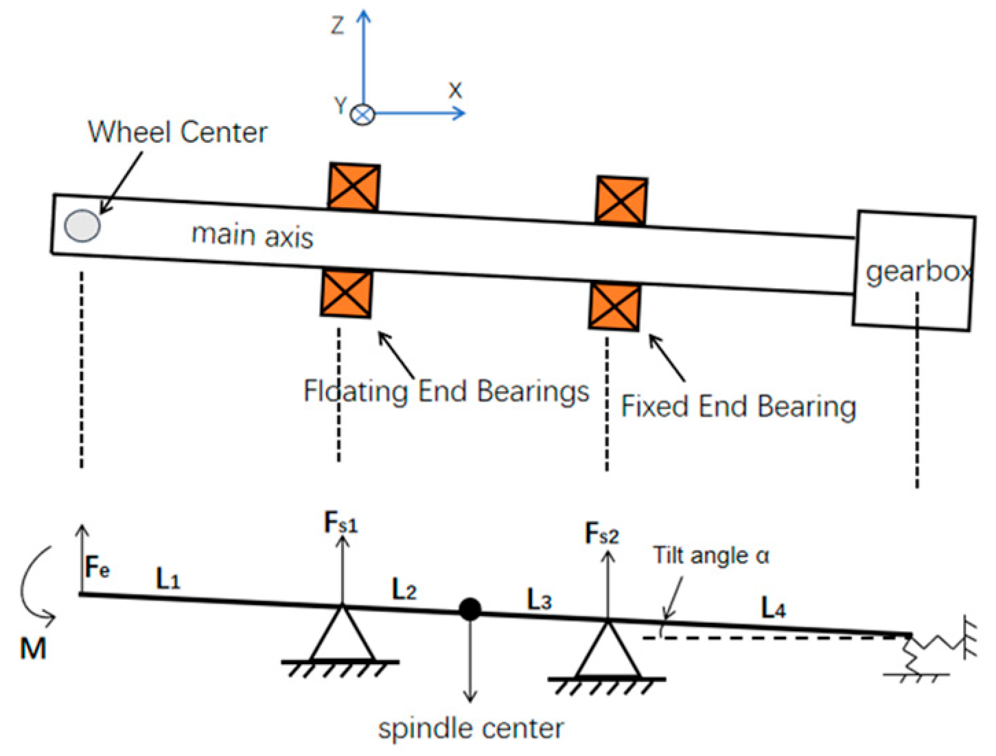
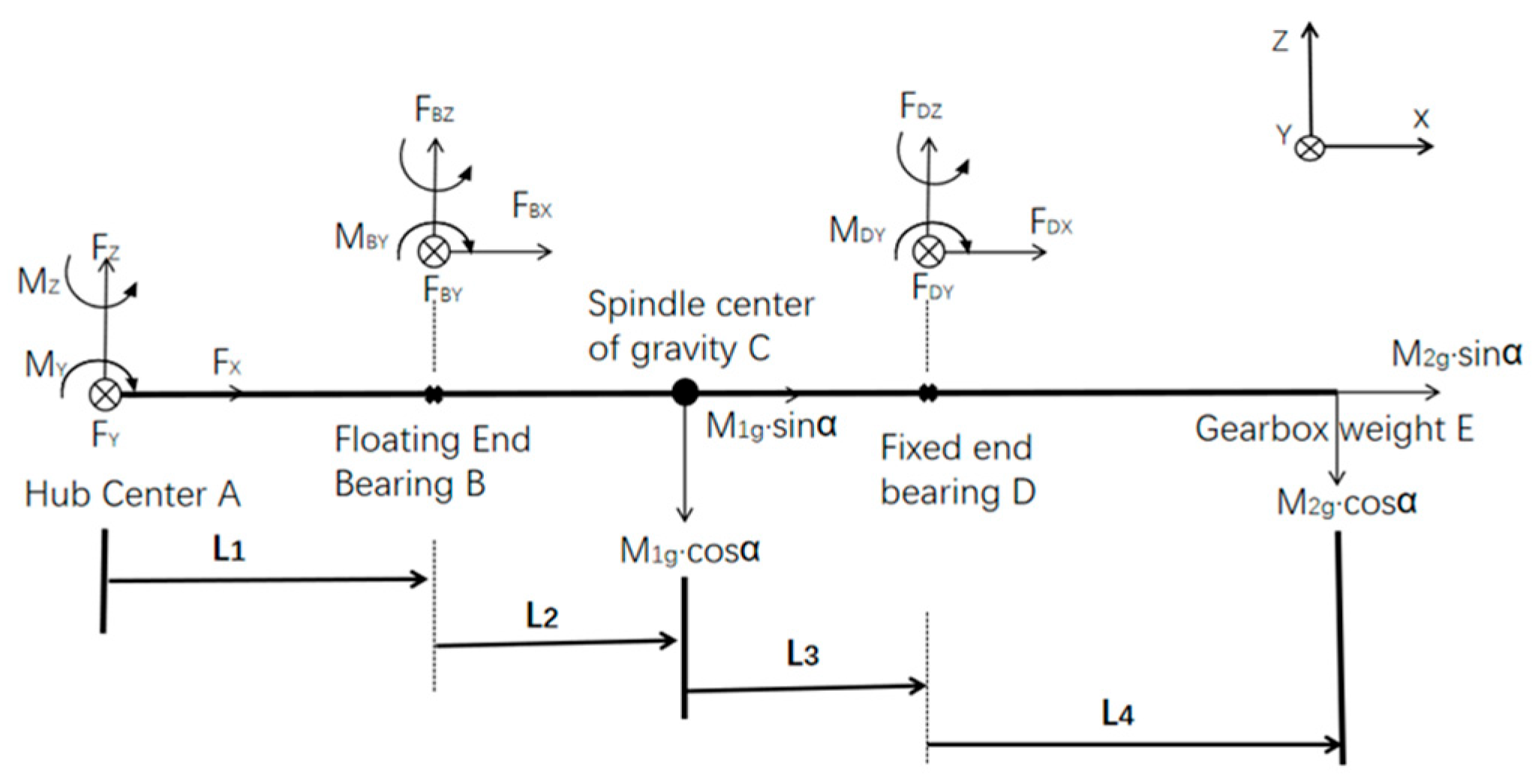
Wind turbine drivetrains typically employ two hub-bearing configurations. The first utilizes a single main bearing, while the second incorporates dual bearing rows arranged in a straddle-mounted or downwind configuration. Both configurations demonstrate analytical equivalence, though this study focuses on the more prevalent straddle-mounted arrangement. As main shafts typically incorporate a tilt angle, we decompose the 5-degree-of-freedom hub load sequence into orthogonal Cartesian components relative to the shaft coordinate system for enhanced analytical clarity. The hub center coordinates, spindle system layout, and stress analysis are shown in Figure 1, Figure 2 and Figure 3.
Balance equation along the X axis:
F X + F B X + F D X + M 1 g sin α + M 2 g sin α = 0
Balance equation along the Y axis:
F X + F B X + F D X + M 1 g sin α + M 2 g sin α = 0
Balance equation along the Z axis:
F Z + F B Z + F D Z M l g c o s α M 2 g cos α = 0
Take the rectangle at point A, and the equilibrium equation around the Y-axis:
M Y + F B Z L 1 + M l g cos α L 1 + L 2 F D Z L 1 + L 2 + L 3 + M 2 g cos α L 1 + L 2 + L 3 + L 4 = 0
Take the moment of A point, and the equilibrium equation around the Z axis:
M Z + F B Y L 1 + F D Y L 1 + L 2 + L 3 = 0
Radial force F a on the fixed-end bearing of the spindle:
F r = F D Y 2 + F D Z 2
Axial force   F a on the fixed-end bearing of the spindle:
F a = F D X
Radial force F f r on the floating-end bearing of the spindle:
F f r = F B Y 2 + F B Z 2
Since the floating-end bearing of the spindle does not bear axial force, its axial force F f a   = 0. The hub load, torque, spindle drive system size, and other data can be put into the Formulas (26)–(33) to calculate the fixed-end bearing random wind speed axial load and radial load. Similarly, the axial load and radial load under random wind speed can be calculated for the floating-end bearing.

2.4. Theoretical Calculation of Internal Load Distribution of Main Bearings

Spherical roller bearings in the form of double rows of rollers can withstand strong radial loads and some axial loads. Due to the lack of constraint relationship between the inner and outer rings, spherical roller bearings cannot withstand moment effects [19]. In order to analyze the roller-raceway contact force and the corresponding displacement of the bearing under external load, the global and local coordinate system of the bearing established by taking the center of the outer ring and the center of each roller as the origin, respectively, F = [Fx,Fy,Fz] is the external load applied to the inner ring of the bearing, and δ = [δx,δy,δz] is the corresponding displacement of the inner ring under the action of each load. The parametric model of the ROMAX main bearing is shown in Figure 4.
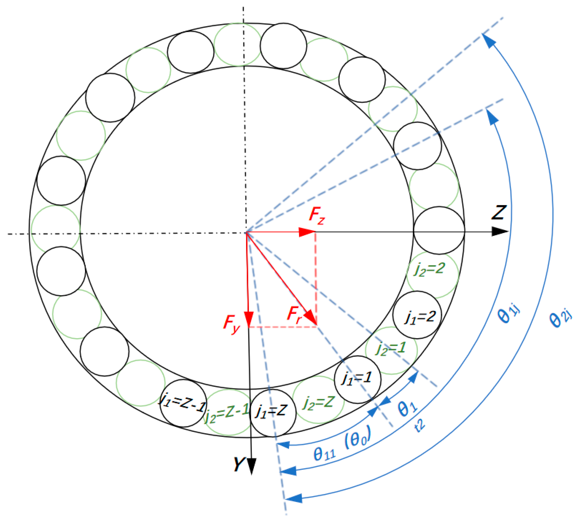
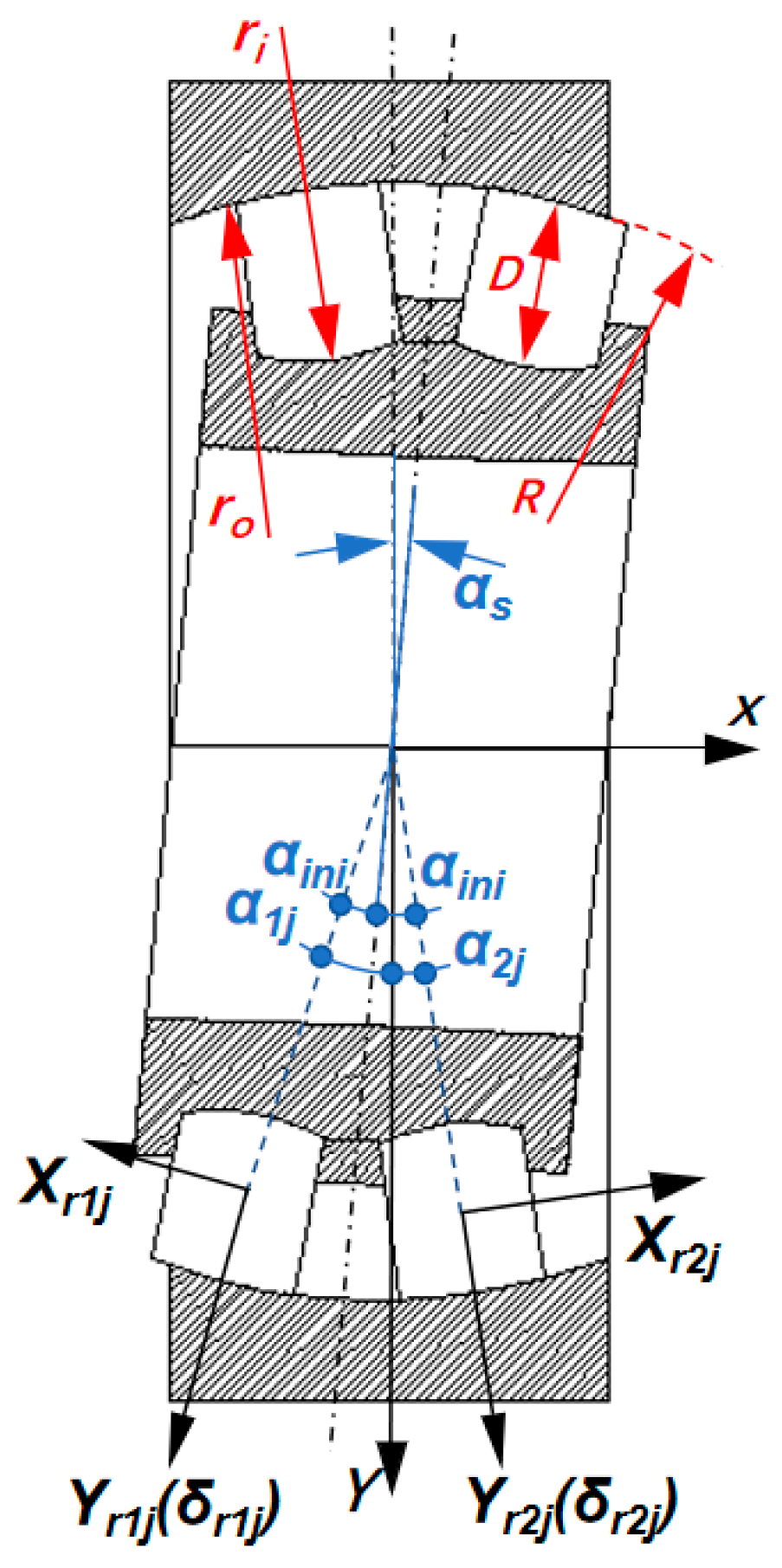
The rollers of self-aligning roller bearings come into contact with the inner and outer rings via spherical raceways. When there is an angular misalignment between the inner and outer rings, a certain inclination angle is generated between their radial cross-sections, thereby achieving automatic self-alignment [20]. For convenience in calculation, it is specified that, when the inner ring is offset in the clockwise direction as shown in the figure, the self-aligning angle   α s is positive; otherwise, it is negative. The arrangement of rollers in self-aligning roller bearings can be either parallel or staggered, meaning that there may be an offset angle θ 1 t 2 between the first and second rows of rollers. Bearing roller numbering, position angle, and local coordinate system, as shown in Figure 5 and Figure 6.
Specify the roller number 1/2j and then the position angle of the jth roller in the 1st and 2nd columns:
θ 1 j / 2 j = 2 π Z j 1 + θ 0 + θ 1 t 2
In the formula, the interlacing angle θ 1 t 2 is only effective for the position angle of the second column of rollers.
Based on geometric relationships, the displacement of the jth axial section of the inner ring raceway along the Yr1j/r2j axis can be obtained.
δ i 1 j = δ y c o s α 1 j c o s θ 1 j + δ z c o s α 1 j s i n θ 1 j δ x s i n α 1 j δ i 2 j = δ y c o s α 2 j c o s θ 2 j + δ z c o s α 2 j s i n θ 2 j + δ x s i n α 2 j
In the formula, α 1 j and α 2 j   are the contact angles of the jth roller in the 1st and 2nd columns, respectively.
When the bearing generates an alignment angle   α s , the contact angles α 1 j / 2 j of each roller will change with different position angles   θ 1 j / 2 j , specifically as follows:
α 1 j / 2 j = α i n i + 2 θ 1 j ± π π α s , 0 θ 1 j / 2 j π α i n i + ± 2 θ 1 j 3 π π α s , π < θ 1 j / 2 j < 2 π
In the formula, the upper and lower symbols are used for the first and second columns of rollers, respectively.
When the inner ring of the bearing undergoes displacement in the global coordinate system, the rollers also undergo corresponding motion. Therefore, the relative displacements between the jth roller in the first and second rows and the inner and outer ring raceways are, respectively,
δ i r 1 j / i r 2 j = δ i 1 j / i 2 j δ r 1 j / r 2 j δ o r 1 j / o r 2 j = δ r 1 j / r 2 j
In the equation, δr1j and δr2j represent the displacement of the jth roller in the 1st and 2nd columns along the Yr1j and Yr2j axes, respectively. The subscripts i and o represent the inner and outer rings, respectively.
Further, the normal contact deformation between the jth roller in columns 1 and 2 and the inner and outer ring raceways can be obtained as follows.
δ i 1 j p / o 1 j p / i 2 j p / o 2 j p = δ i r 1 j / o r 1 j / i r 2 j / o r 2 j P d 4 c o s α 1 j / 2 j
In the formula, P d is the radial clearance of the self-aligning roller bearing, which is taken as 0.398 in this paper.
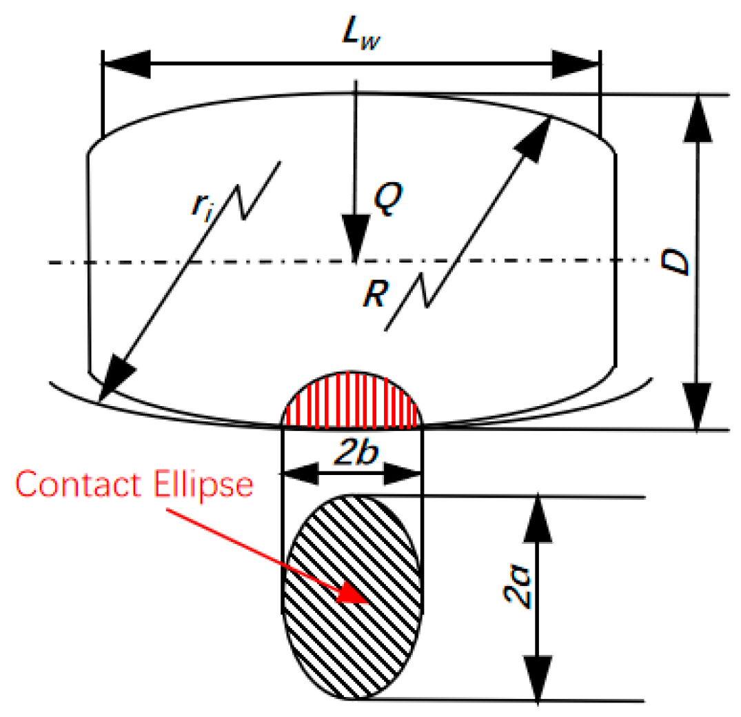
The raceway of the roller contacts the ellipse as shown in Figure 7. According to Hertz point contact theory [21], the normal contact loads between the jth roller in the first and second rows of the bearing and the inner and outer ring raceways are respectively
Q i 1 j / i 2 j = K i δ i 1 j p / i 2 j p 3 2 Q o 1 j / o 2 j = K o δ o 1 j p / o 2 j p 3 2
In the equation, K i and K o are the contact stiffness coefficients of the inner and outer ring raceways and rollers, respectively. If the calculated values of δi1jp/i2jp and δo1jp/o2jp are negative, it indicates that the rollers are not loaded, and the corresponding Qi1j/i2j and Qo1j/o2j should be set to zero.
Where Ki and Ko can be expressed as
K i / o = 2.0678 π 3 ( 1 ν i / o 2 E i / o + 1 ν r 2 E r ) 2.0006 + 1.1936 ( R i r x / o r x R i r y / o r y ) ( R i r y / o r y R i r x / o r x ) 1.272 1.5277 + 0.6023 l n ( R i r y / o r y R i r x / o r x ) 3 ρ i r / o r
In the equation, ν i / o , E i / o , and E r are the Poisson’s ratios and elastic moduli of the inner and outer rings and rollers, respectively. R i r x / o r x and R i r y / o r y are the equivalent radii of the contact ellipse between the inner and outer rings and rollers in the long and short semi-axis directions, respectively. ρ i r / o r are the principal curvatures at the contact points between the inner and outer rings and rollers, and the equivalent radii at the contact points between the inner and outer ring raceways and rollers, respectively.
1 R i r x / o r x = ± 2 γ D ( 1 γ ) + 2 D 1 R i r y / o r y = 1 r i / o + 1 R
r i / o = R + Δ i / o
ρ i r / o r = ± 2 γ D ( 1 γ ) 1 r i / o + 2 D + 1 R
In the equation, the symbols i and o are used to denote the inner and outer rings, respectively. Δ i / o represents the curvature difference between the inner and outer raceways and the rollers, typically ranging from 2% to 5% of the roller radius. The specific value should be adjusted based on load, material, and bearing type; in this paper, a value of 3% is adopted.
In the equation, the upper and lower symbols represent the inner and outer rings, respectively. D is the roller diameter, and R, ri, and ro are the contour radii of the roller, inner ring, and outer ring raceways in the axial cross-section, respectively. γ is defined as
γ = Dcos α i n i d m
In the equation, α i n i   is the initial contact angle of the bearing, and d_m is the pitch diameter.
The self-aligning roller bearings used in this paper are for the main shaft of wind turbines. The inner ring speed is low, and the centrifugal force generated by the circumferential motion can be neglected, i.e., the normal contact loads between the inner and outer ring raceways and the rollers are approximately equal. The equilibrium equations for the jth roller in the first and second rows can be listed as follows:
Q i 1 j Q o 1 j = 0 Q i 2 j Q o 2 j = 0
At the same time, the normal contact load of the roller on the inner ring should be balanced with the external loads Fx, Fy, and Fz. The overall balance equation of the bearing can be listed as follows:
F x + j = 1 Z   Q i 1 j s i n α 1 j j = 1 Z   Q i 2 j s i n α 2 j = 0 F y j = 1 Z   Q i 1 j c o s α 1 j c o s θ 1 j j = 1 Z   Q i 2 j s i n α 2 j c o s θ 2 j = 0 F z j = 1 Z   Q i 1 j c o s α 1 j s i n θ 1 j j = 1 Z   Q i 2 j s i n α 2 j s i n θ 2 j = 0
Obviously, the system of simultaneous equations in Equations (45) and (46) contains 2Z+3 unknowns, which is a relatively large number. The Newton–Raphson iteration method can be used to solve the above system of equations.

2.5. Theory of Fatigue Life Calculation for Self-Aligning Roller Bearings

Fatigue life analysis of rolling bearings is a critical component of bearing design. In the 1940s, Lundberg and Palmgren proposed the L-P theory for the fatigue life of rolling bearings, which serves as one of the foundational theories for predicting the fatigue characteristics of rolling bearings and is commonly used to analyze their fatigue properties [22]. Although subsequent material and process innovations led to the simplification of standards, resulting in the international standard ISO 281 [23], its simplified model ignores differences in load distribution between rolling elements, leading to limitations in life estimation. Therefore, this paper still adopts the L-P theory to calculate bearing life, in order to more accurately characterize the influence of contact stress gradients on fatigue damage. Its expression is as follows:
L 10 = C P p
In the formula, L 10 is the 90% reliability life, C is the rated dynamic load, and P is the equivalent load; p = 3 for ball bearings and p = 10/3 for roller bearings. This theory unifies the material fatigue mechanism, stress field distribution, and statistical failure probability for the first time.
Based on the statistical failure model of L-P theory and the characteristics of the Weibull distribution, the fatigue life expression for double-row self-aligning roller bearings with point contact characteristics is as follows:
L = ( L 1 10 9 + L 2 10 9 ) 9 10
In the formula, L1 and L2 are the fatigue lives of the rollers and raceways in the first and second rows, respectively, and are generally measured in millions of revolutions.
The roller-raceway life of each row of self-aligning roller bearings can be calculated using the fatigue life formula for single-row point-contact bearings, i.e.,
L 1 / 2 = ( L 1 i / 2 i 10 9 + L 1 e / 2 e 10 9 ) 9 10
In the formula, L1i, L2i, L1e, and L2e are the fatigue life of the inner and outer raceways of columns 1 and 2, respectively.
Considering the contact area characteristics of the material, the fatigue limit stress, and the average stress, the fatigue life of each contact point on the inner raceway can be calculated using the following formula [24]
N 1 i j / 2 i j = C α σ 1 i j m a x / 2 i j m a x 1 R 1 i / 2 i 2 σ 1 i a c , e / 2 i a c , e β
α = 2 σ s σ s + σ 0
Among them, C and β are material constants. σ i j m a x represents the maximum contact stress at each contact point between the roller and the inner raceway. σ a c , e is the equivalent stress amplitude. R is the stress ratio, σ s   is the yield strength, and σ 0 is the yield strength of similar materials when the average stress sensitivity coefficient is 0.5.
Since the contact stress at any point on the inner raceway varies periodically with the rotation of the inner ring, it can be calculated using Miner’s linear damage accumulation criterion. The Miner criterion states that, when a series of cycles are subjected to different stress amplitudes σ1, σ2, σ3, …, the fatigue life corresponding to each stress amplitude is N f 1 , N f 2 , N f 3 , …, and the actual number of cycles is N1, N2, N3, …, the fatigue life consumed under each stress amplitude is the actual number of cycles   N k divided by the life cycle N f k , i.e., N k / N f k [25]. The total damage value for the entire operational process of the component can be obtained by accumulating the damage values from all stress cycles, i.e.,
N 1 N f 1 + N 2 N f 2 + N 3 N f 3 + = k = 1   N k N f k = 1
For the sake of convenience in research, the engineering field has integrated the macro framework of fatigue damage accumulation with the micro mechanism of local stress analysis in bearings, combining Miner’s linear damage accumulation theory with the L-P bearing fatigue theory [24]. Since the number of rolling elements is not unique, u i   can be used to represent the number of rolling elements passing through a certain point on the inner ring when the inner ring rotates one revolution. The fatigue damage caused by the inner ring can then be expressed as:
D 1 i / 2 i = j = 1 u 1 i / 2 i   1 N 1 i j / 2 i j u 1 i / 2 i
Then, calculate the fatigue life of the inner ring using the following formula:
L 1 i / 2 i = 1 D 1 i / 2 i = 1 j = 1 u 1 i / 2 i   1 N 1 i j / 2 i j u 1 i / 2 i
The maximum contact stress on the outer raceway occurs at the 0-degree position angle. Therefore, it can be assumed that the fatigue life at this point is equal to the fatigue life of the outer ring, i.e.,
L 1 e / 2 e = N 1 e / 2 e u 1 e / 2 e
N 1 e / 2 e = C α σ 1 e m a x / 2 e m a x 1 R 1 e / 2 e 2 σ 1 e a c , e / 2 e a c , e β
Among them, σ e m a x   is the maximum contact stress on the outer raceway. u e   represents the number of rolling elements passing through a certain point on the outer ring when the inner ring rotates one revolution.
Similarly, based on the stress–strain interference theory, the cumulative damage analysis method is used to analyze the fatigue life of rolling bearings. When the cumulative fatigue damage is less than the critical damage, the bearing can operate normally; otherwise, it is considered to be fatigue failure [26]. The fatigue limit state function is created as:
G = D c D = D c t R v
In the equation, R(v) represents the bearing’s lifespan under the influence of the random variable v w , t u r b ,, and D c   is the lifespan threshold. According to the GL wind turbine industry design standards, the operational lifespan of the main shaft bearings in wind turbines should reach 20 years [27]. Based on an average main shaft speed of 12 r/min, the converted result is   D c   = 105.12 × 10⁶ revolutions. When G < 0, the bearing fatigue life is below the specified threshold.
P f 0 , T = P G v w , t u r b , D t , t < 0 , t 0 , T
The overall calculation method for predicting the fatigue life of a self-aligning roller bearing with a fixed shaft end under random wind speeds is shown in the Figure 8.

3. Case Study and Discussion

This study takes the 4.5 MW wind turbine as the research object, the main shaft support type is a two-point support, near the hub end is a floating-end bearing, near the gearbox end is a fixed-end bearing, and both main shaft bearings are double row spherical roller bearings. The spindle system parameters are shown in Table 2. The spherical roller bearings installed in the main shaft are FD-240/800X3/HC W33 (Luoyang, China) double-row spherical roller bearings (fixed-end bearing of the main shaft) and FD-249/1060CA/HC W33 (Luoyang, China) double-row spherical roller bearings (floating-end bearing of the main shaft). There are no models of the two main bearings in the Romax bearing library, so it is necessary to input the parameters of the two bearings to establish the parameterization of the fixed-end and floating-end bearings. The parameters of the fixed-end and floating-end bearings are shown in Table 3 and Table 4, and the simulation model of the two bearings in Romax is shown in Figure 9. In Romax, the materials of the fixed-end and floating-end bearings of the spindle are defined: the rollers and inner and outer rings of the two bearings are of the same material, both of which are G20Cr2Ni4A, with a density of 7.82 g/cm3 [28].
The technical parameters of the bearings and typical operating conditions of a 4.5 MW wind turbine generator are as follows:

3.1. Analysis of Main Shaft Speed Under Random Wind Speeds

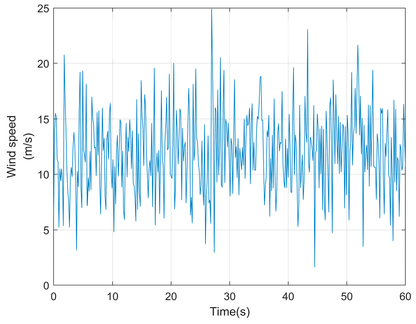
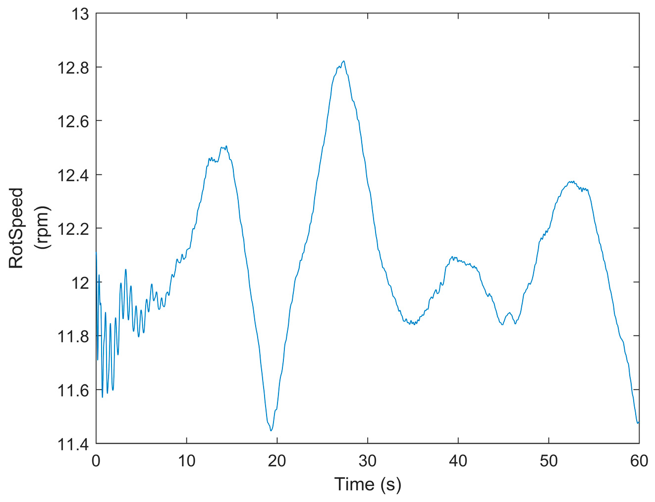
Combining the turbulent wind speed model from Section 2.1, a turbulent wind speed curve with an average wind speed of 12 m/s and turbulence intensity of Class B was generated, as shown in Figure 10. To further analyze the turbulence wind speed model, a traditional two-parameter Weibull distribution wind speed model was introduced for comparative analysis. Based on Reference [29], a random wind speed curve with an average wind speed of 12 m/s and a wind speed variance of 14 m2/s2 was generated, as depicted in Figure 11. Based on the content of Section 2.2 and Section 2.3, aerodynamic elasticity theory, and the structural information of the wind turbine, a main shaft rotational speed curve was generated under these random wind speed conditions, as shown in Figure 12.
Analysis of Figure 10, Figure 11 and Figure 12 shows that:
(1)
It can be observed that the curve of the traditional two-parameter Weibull wind speed model exhibits significant local fluctuations, yet its overall variation remains relatively small. It does not display the gradual, smooth trend characteristic of long-term wind speed monitoring. In contrast, the turbulence wind speed model curve shows smaller local fluctuations but exhibits smoother overall variation with a distinct trend.
(2)
Wind speed increased from 11 m/s to 13 m/s between 10 and 25 s, with the rotational speed increasing synchronously from 12.0 rpm to 12.4 rpm; 40–50 s: Wind speed decreases, and rotational speed drops. This indicates that the main shaft rotational speed is significantly correlated with turbulent wind speed in the mid-to-low frequency range. Large-scale turbulent changes directly drive rotational speed changes, reflecting the dominant role of aerodynamic torque in energy capture. Turbulent wind speed and wind turbine main shaft rotational speed exhibit frequency-domain selective coupling—large-scale turbulence dominates the energy capture trend.
(3)
The wind speed curve exhibits sawtooth-like fluctuations within 0–10 s, but the rotational speed curve is smoother (with significantly compressed fluctuation amplitude). This is because the inertia of the transmission chain and MPPT control work together to suppress high-frequency disturbances, compressing the rotational speed fluctuation amplitude to 24% of the wind speed. This mechanism is consistent with the intrinsic laws of stable operation of wind turbines in random wind fields [30]. The correctness of the aerodynamic load calculation model proposed in this paper has been demonstrated, and it also provides a theoretical foundation for dynamic load prediction and control optimization of the transmission system.

3.2. Hub Center Load Analysis

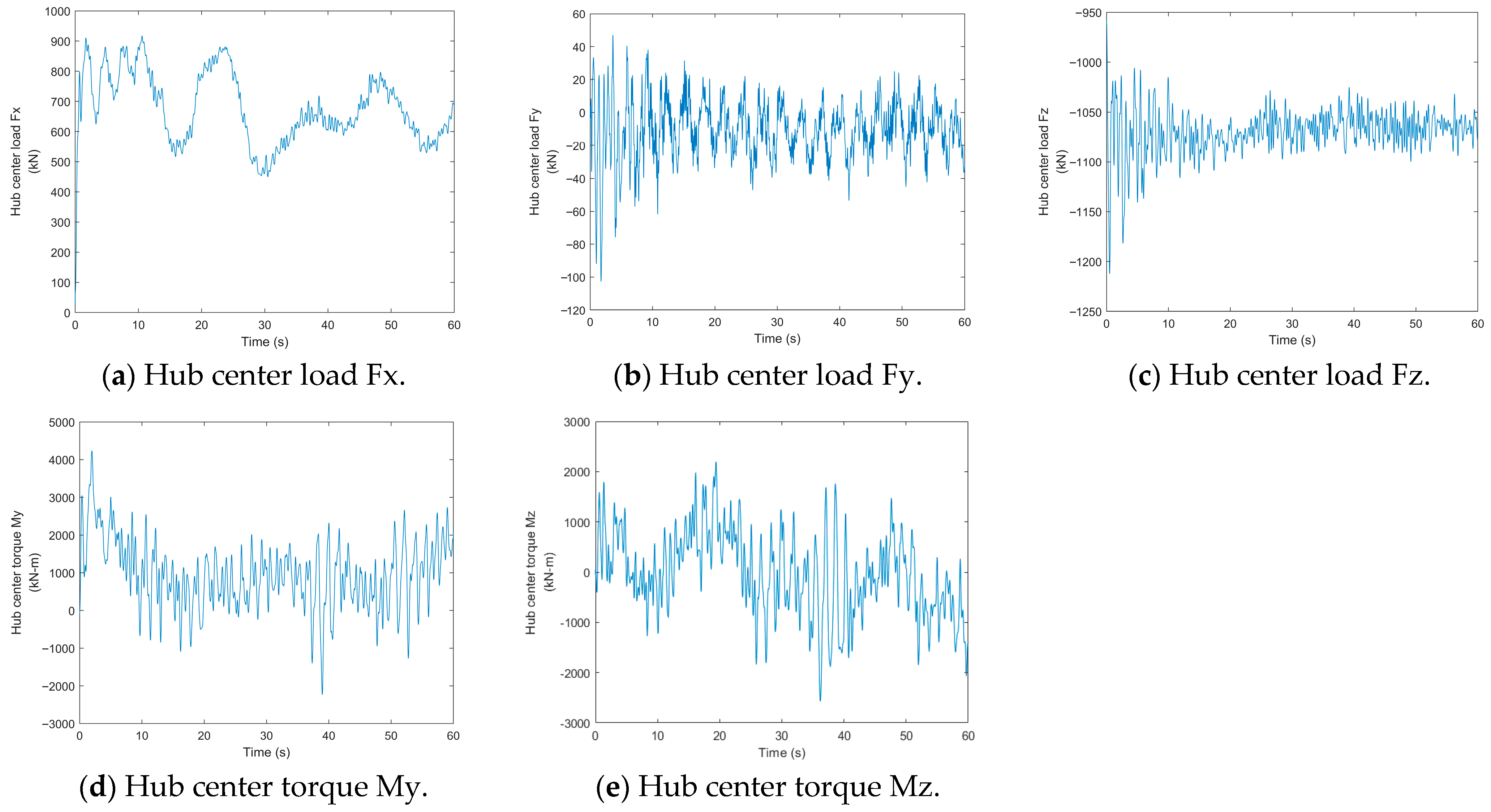
Using MATLAB R2020a software, the time-series wind speed generated by the turbulent wind speed model is input into the theoretical model in Section 2.2 for aeroelastic simulation. The aim is to extract the hub center loads with five degrees of freedom from the random wind speed for the wind turbine, namely Fx, Fy, Fz, My, and Mz. The time-series load curves are shown in the Figure 13.
From the curves of the hub center load for the five degrees of freedom in Figure 13, it can be observed that the hub center load Fy curve has the smallest fluctuation range, approximately 60 kN, but a higher fluctuation frequency. The hub center load Fx curve has the lowest fluctuation frequency but a higher fluctuation amplitude. The fluctuation trajectory of the hub center torque Mz curve between 10 and 50 s exhibits a high degree of similarity to the random wind speed curve in Figure 10, while the fluctuation of the hub center torque My curve between 20 and 50 s is relatively small. Overall, the fluctuation range of the hub center load across the five degrees of freedom in Figure 13 is relatively small. However, the local numerical fluctuations are greater than those in Figure 10 and Figure 12, indicating that wind speed variations exert a more pronounced influence on the hub center load.

3.3. Verification of the Evaluation of Main Bearing External Loads

First, the hub center loads in Section 2.2 are randomly sampled, and finally summarized into the fatigue load spectra of 16 working conditions, as shown in the following Table 5:
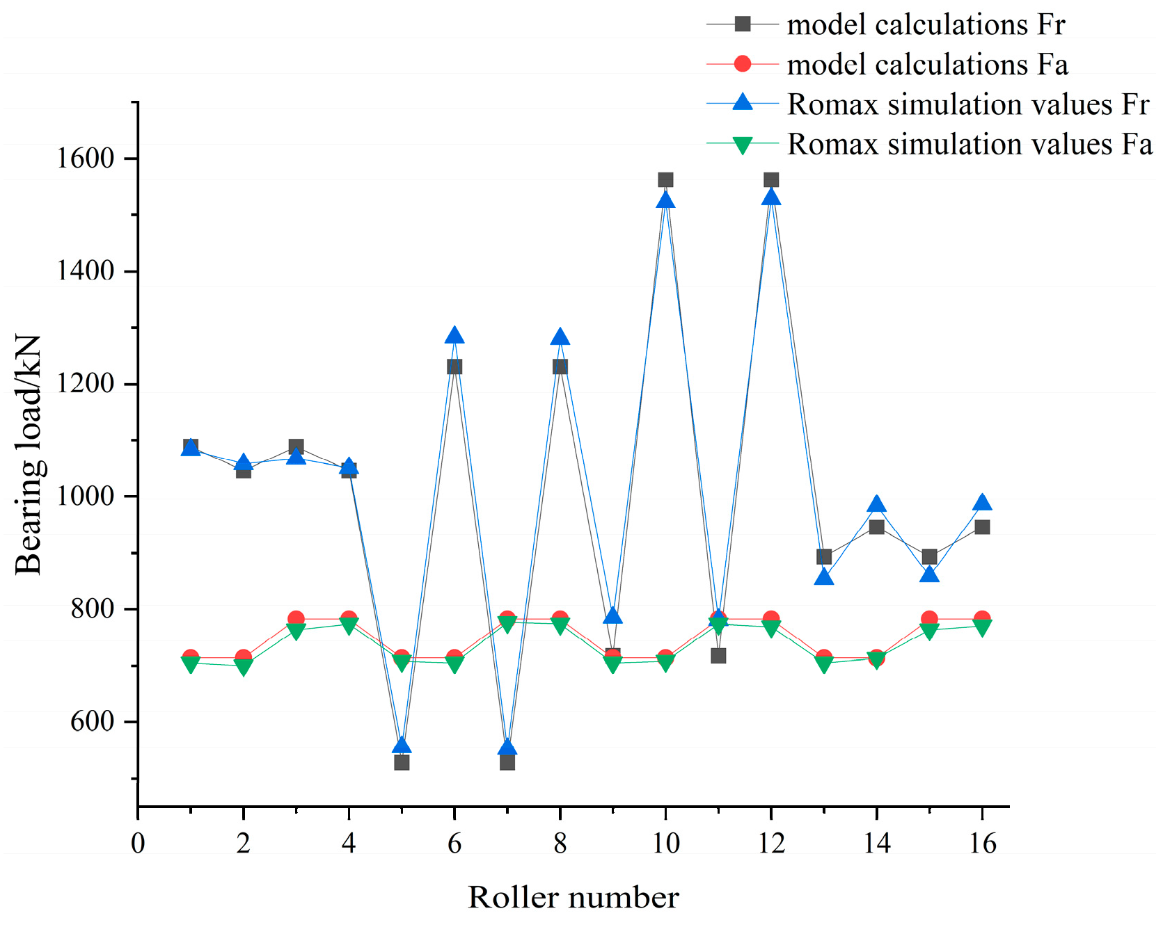
Subsequently, combined with the main shaft structural parameters and formulas (26)–(32), theoretical calculations and Romax simulation calculations were carried out respectively. Finally, the theoretical calculation results under the 16 working conditions were compared with the Romax results (as shown in the Figure 14), and it can be found that the two sets of calculation results are almost identical.

3.4. Verification and Analysis of the Roller-Raceway Normal Contact Load Model

The results of the analysis of the normal contact load between the roller and raceway of the fixed-end bearing using the theoretical model introduced in Section 2.4 of this paper are compared with those obtained using the industry-standard analysis software Romax. This comparison aims to demonstrate that the contact load model for the roller-raceway interface of self-aligning roller bearings exhibits high accuracy. When using dynamic spindle speed as the input, the computational load is significant. To simplify calculations and result analysis, this section sets the spindle speed to 12 rpm, with the axial load Fx of the fixed-end bearing at 200 kN, and radial loads Fy and Fz at 500 kN and 300 kN, respectively. The calculation results for both are shown in the Figure 15.
Analysis of the differences in roller loads between the two rows, as well as the comparison between the theoretical model and the calculation results from Romax software, reveals that the normal contact loads of the rollers in the second row are generally higher than those in the first row. The maximum contact loads for the first and second rows are 73.82 kN and 233.71 kN, respectively. The average error does not exceed 0.5%, indicating good fitting performance, which demonstrates that the contact load model for the rollers and raceways of self-aligning roller bearings has high accuracy.

3.5. The Effect of Average Wind Speed and Turbulence Intensity on Fatigue Life

Three wind farms (i.e., 12-A, 12-B, and 14-A) with average wind speeds (12 rpm and 14 rpm) and turbulence intensities (Class A and Class B) were used to simulate the aeroelasticity of wind turbines. Then, based on the theoretical method proposed in Section 2.5, a failure probability analysis and fatigue life prediction were performed on the main bearing, with the results shown in the figure.
Figure 16a, Figure 16b, and Figure 16c are, respectively, the histograms of the failure probability of the main bearing under random wind speeds with an average wind speed corresponding to 12 rpm or 14 rpm and a turbulence intensity of Class A or Class B. The ordinate represents the probability, and the abscissa represents the number of rotations that the bearing should achieve within 20 years at the rotational speed generated by the corresponding wind speed. The red color indicates fatigue failure of the bearing (i.e., its fatigue life is less than 20 years), while the blue color indicates no fatigue failure.
Comparing Figure 16a and Figure 16c, respectively, the probability distribution of fatigue life shows significant differences for different average wind speeds. In Figure 16a, the probability of fatigue failure is generally below 4%, while in Figure 16c, the probability of fatigue failure is mostly above 8%. This indicates that, within a certain range, wind farms with higher average wind speeds have lower bearing failure probabilities, and average wind speed significantly affects fatigue life and failure probability. Therefore, the probability of fatigue life is closely related to average wind speed and decreases as average wind speed increases.
Comparing Figure 16a and Figure 16b, respectively, the probability distribution of fatigue life remains generally similar across wind farms with different turbulence intensities. However, the probability of bearing fatigue failure in Figure 16b is lower than in Figure 16a. This implies that turbulence intensity has a relatively minor impact on the average level of fatigue life, but higher turbulence intensity does increase the probability of bearing fatigue failure.
Utilizing an integrated framework of turbulent wind speed modeling, blade element momentum theory, bearing dynamics, and L-P-Miner fatigue analysis, the calculated fatigue life of the double-row spherical roller bearing at the fixed end of the wind turbine main shaft is 28.8 years under stochastic wind conditions (average wind speed: 12 m/s, turbulence intensity class B). This result falls within the predicted lifespan range of 25.45 to 30.59 years reported in reference [28]. Consequently, the proposed methodology demonstrates validity for predicting main bearing fatigue life in wind turbines operating under stochastic wind fields.

4. Conclusions

In order to solve the problem of complex operating conditions and difficulty in accurately describing the dynamic characteristics of wind turbine main shaft drive system bearings, this study takes the 4.5 MW wind turbine main shaft fixed-end double-row spherical roller bearings as the main research object; establishes a random wind speed model, a pneumatic load model, and a bearing fatigue life prediction model, combining it with the roller-raceway contact load calculation model; and proposes a method for predicting the fatigue life of wind turbine main bearings in a random wind field. The load fluctuation caused by random wind speed in the main shaft drive system of WTGs, and the influence of average wind speed and turbulence intensity on the fatigue life of the main bearings of high-power WTGs are investigated, which is of great theoretical and engineering significance for improving the operational reliability of WTGs. However, this study has not yet explored the specific wind speed range in which the probability of fatigue failure increases when the average wind speed decreases, nor has it examined the effects of other environmental factors (such as temperature and humidity) besides wind speed. This is one of the directions for the author’s future research.
Based on the comprehensive analysis in this paper, the following conclusions can be drawn:
(1)
Average wind speed significantly affects the overall level of fatigue life. Within a certain range, the probability of fatigue failure of the main bearing increases with a decrease in the average wind speed.
(2)
The effect of wind speed fluctuations on the hub center load is more pronounced than that of the spindle speed.
(3)
An engineering formula for evaluating the fatigue life prediction of main bearings at random wind speeds of wind turbines was obtained, which can be used to evaluate the compatibility of the main bearings and wind turbine structure with the wind field characteristics of the installation site.

Author Contributions

Conceptualization, L.F. and Z.W.; Methodology, L.F.; Validation, L.F.; Writing—Original Draft, L.F.; Project Administration, L.F., Z.W., Y.Y., X.L. and W.S.; Funding Acquisition, Z.W. All authors have read and agreed to the published version of the manuscript.

Funding

This work was supported by three projects: 1. Xinjiang Uygur Autonomous Region Tianchi Talent—Young Doctoral Program: “Research on Key Technologies for Intelligent Maintenance of Wind Turbines Based on Digital Twins,” Project Number: 51052300553. 2. Central Government Guidance for Local Development Project—Research and Development of Key Technologies for Digital Design and Intelligent Manufacturing of Wind Power Equipment, Project Number: ZYYD2025JD07.3. Science and Technology Innovation Leading Talent Program—Intelligent Operation and Maintenance Technologies and Applications for High-End Equipment, Project Number: 2024TSYCLJ0010.

Data Availability Statement

The original contributions presented in this study are included in the article. Further inquiries can be directed to the corresponding author.

Conflicts of Interest

The authors declare no conflicts of interest.

References

  1. Zhang, S.J.; Wu, R. II-GLD Position Scale Model for Reliability Assessment of Rolling Bearing Performance Degradation. Comput. Integr. Manuf. Syst. 2025, 31, 637–646. [Google Scholar] [CrossRef]
  2. Qiao, Z.J.; Zhang, C.L.; Zhang, C.L.; Ma, X.; Zhu, R.H.; Lai, Z.H.; Zhou, S.T. Stochastic Resonance Array for Designing Noise-Boosted Filter Banks to Enhance Weak Multi-Harmonic Fault Characteristics of Machinery. Appl. Acoust. 2025, 236, 110710. [Google Scholar] [CrossRef]
  3. He, Y.B.; Qiao, Z.J.; Xie, B.B.; Ning, S.Y.; Li, Z.C.; Kumar, A.; Lai, Z.H. Two-Stage Benefits of Internal and External Noise to Enhance Early Fault Detection of Machinery by Exciting Fractional SR. Chaos Solitons Fractals 2024, 182, 114749. [Google Scholar] [CrossRef]
  4. Qiao, Z.J.; He, Y.B.; Liao, C.R.; Zhu, R.H. Noise-Boosted Weak Signal Detection in Fractional Nonlinear Systems Enhanced by Increasing Potential-Well Width and Its Application to Mechanical Fault Diagnosis. Chaos Solitons Fractals 2023, 175, 113960. [Google Scholar] [CrossRef]
  5. Li, C.; Chen, Z.; Liu, Z.; Han, X.; Chen, X. A Method for Predicting Subsurface Fatigue Life of Rolling Bearings Based on Macro–Micro Coupling Model. Proc. Inst. Mech. Eng. Part J J. Eng. Tribol. 2021, 236, 1056–1073. [Google Scholar] [CrossRef]
  6. Lu, Y.; Tang, D.; Zhu, D.; Gao, Q.; Zhao, D.; Lyu, J. Remaining Useful Life Prediction for Bearing Based on Coupled Diffusion Process and Temporal Attention. IEEE Trans. Instrum. Meas. 2024, 73, 3510310. [Google Scholar] [CrossRef]
  7. Zhao, L.H.; Li, Q.C.; Feng, J.Z.; Zheng, S.L. Service Life Prediction Method for Wheel-Hub-Bearing Under Random Multi-Axial Wheel Loading. Eng. Fail. Anal. 2021, 122, 105211. [Google Scholar] [CrossRef]
  8. Wang, X.; Meng, Q.; Zhang, T. Sensitivity Analysis of Rolling Bearing Fatigue Life Under Cyclic Loading. J. Mech. Sci. Technol. 2022, 36, 5689–5698. [Google Scholar] [CrossRef]
  9. Cavacece, F.; Frache, L.; Tonazzi, D.; Bouscharain, N.; Philippon, D.; Le Jeune, G.; Maheo, Y.; Massi, F. Roller Bearing Under High Loaded Oscillations: Life Evolution and Accommodation Mechanisms. Tribol. Int. 2020, 147, 106278. [Google Scholar] [CrossRef]
  10. Kong, X.; Ding, H.; Tang, J.; Hu, Z.; Chen, S. Bearing Internal Load Analysis and Fatigue Life Estimation Based on Nonlinear Dynamic Model of a Gear System. J. Vib. Control 2021, 28, 1635–1642. [Google Scholar] [CrossRef]
  11. Jacobs, W.; Van Hooreweder, B.; Boonen, R.; Sas, P.; Moens, D. The Influence of External Dynamic Loads on the Lifetime of Rolling Element Bearings: Experimental Analysis of the Lubricant Film and Surface Wear. Mech. Syst. Signal Process. 2016, 74, 144–164. [Google Scholar] [CrossRef]
  12. Guo, B.; Luo, Z.; Zhang, B.; Liu, Y.; Chen, Z. Dynamic Influence of Wheel Flat on Fatigue Life of the Traction Motor Bearing in Vibration Environment of a Locomotive. Energies 2021, 14, 5810. [Google Scholar] [CrossRef]
  13. Gao, T.; Li, Y.; Huang, X.; Wang, C. Data-Driven Method for Predicting Remaining Useful Life of Bearing Based on Bayesian Theory. Sensors 2021, 21, 182. [Google Scholar] [CrossRef] [PubMed]
  14. Ying, J.; Yang, Z.; Chen, C.; Liu, Z.; Li, S.; Chen, H. Remaining Useful Life Prediction of Rolling Element Bearing Based on Hybrid Drive of Data-Driven and Dynamic Model. Proc. Inst. Mech. Eng. Part C J. Mech. Eng. Sci. 2022. [Google Scholar] [CrossRef]
  15. Guo, R.; Wang, Y. Remaining Useful Life Prognostics for the Rolling Bearing Based on a Hybrid Data-Driven Method. Proc. Inst. Mech. Eng. Part I J. Syst. Control Eng. 2020, 235, 517–531. [Google Scholar] [CrossRef]
  16. Li, P.H.; Yuan, Y. Site-Specific Assessment: Key Guarantee for Wind Turbine Reliability. Qual. Certif. 2025, S1, 99–104. [Google Scholar]
  17. Wang, M.M.; Cui, Q.W.; Cao, L.; Zhou, J.X.; Wen, J.M. Dynamic Characteristics of High-Speed Stage Bearings in Wind Turbine Gear Transmission Systems. Bear 2024, 12, 46–53. [Google Scholar] [CrossRef]
  18. Wang, H. Progressive Damage Analysis and Fatigue Life Reliability Assessment of Composite Wind Turbine Blades. Ph.D. Dissertation, University of Electronic Science and Technology of China, Chengdu, China, 2025. [Google Scholar]
  19. Liu, X.J.; Liu, L.; Xu, H.; Zhang, S.; Xing, Y. Influence of Roller Distribution on Service Performance of Spherical Roller Bearings. J. Xi’an Jiaotong Univ. 2018, 52, 9–17. [Google Scholar]
  20. Huang, X.Z.; Chen, S.J.; Jiang, Z.Y. Contact Load and Life Reliability Analysis of Wind Power Spherical Roller Bearings. J. Jilin Univ. (Eng. Technol. Ed.) 2025. [Google Scholar] [CrossRef]
  21. Luo, J.W.; Luo, T.Y. Analysis, Calculation and Application of Rolling Bearings; Mechanical Industry Press: Beijing, China, 2009. [Google Scholar]
  22. Zhao, Y. Research on Rolling Contact Fatigue Life Prediction Model of Bearing Steel and Its Application. Ph.D. Dissertation, Beijing Jiaotong University, Beijing, China, 2024. [Google Scholar] [CrossRef]
  23. ISO 281:2007; Rolling Bearings—Dynamic Load Ratings and Rating Life. International Organization for Standardization: Geneva, Switzerland, 2007.
  24. Yu, A.; Ruan, R.; Zhang, X.; He, Y.; Li, K. Reliability Analysis of Rolling Bearings Considering Failure Mode Correlations. Qual. Reliab. Eng. Int. 2024, 40, 3079–3095. [Google Scholar] [CrossRef]
  25. Du, K.L.; Wang, Y.S.; Fan, X.G. Fatigue Calculation Analysis of Mooring Structure for FPSO. Val. Eng. 2025, 44, 25–28. [Google Scholar]
  26. Wang, C. Structural Design of Eddy-Current Tuned Roller Damper and Vibration Reduction Performance for Wind Turbines. Ph.D. Dissertation, Huazhong University of Science and Technology, Wuhan, China, 2024. [Google Scholar] [CrossRef]
  27. Li, L.; Niu, B.Z.; Jin, X.Y.; Lian, S.W. Reliability Assessment Method for Wind Turbine Main Bearing Life. J. Mech. Des. Manuf. 2025, 1–6. [Google Scholar] [CrossRef]
  28. Niu, B.Z. Fatigue Life and Reliability Analysis of Wind Power Spherical Roller Main Bearings. Master’s Thesis, Henan University of Science and Technology, Luoyang, China, 2022. [Google Scholar] [CrossRef]
  29. Liu, X.; Wu, Z.; Yuan, Y.; Sun, W.; Gao, J. Reliability Modeling of Wind Turbine Gearbox System Considering Failure Correlation Under Shock–Degradation. Sensors 2025, 25, 4425. [Google Scholar] [CrossRef] [PubMed]
  30. Chai, Y.F. Influence of Turbulent Coherent Structures in Hexi Atmospheric Boundary Layer on Wind Turbine Aerodynamic Performance. Ph.D. Dissertation, Lanzhou University of Technology, Lanzhou, China, 2023. [Google Scholar]
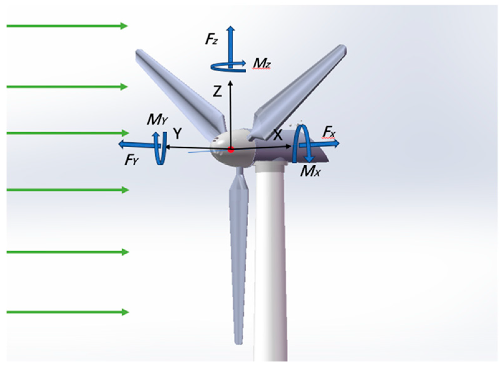
Figure 1. Diagram showing the center coordinates of the wheel hub.
Machines 13 00907 g001
Figure 2. Layout diagram of the main shaft system.
Machines 13 00907 g002
Figure 3. Simplified diagram of the force analysis of the main shaft.
Machines 13 00907 g003
Figure 4. ROMAX main bearing parametric model.
Machines 13 00907 g004
Figure 5. Bearing roller numbers and position angles.
Machines 13 00907 g005
Figure 6. Local coordinate system.
Machines 13 00907 g006
Figure 7. The raceway of the roller contacts the ellipse.
Machines 13 00907 g007
Figure 8. Overall calculation flowchart.
Machines 13 00907 g008
Figure 9. Romax Wind Turbine Spindle Model.
Machines 13 00907 g009
Figure 10. Turbulent Wind Speed 12-B.
Machines 13 00907 g010
Figure 11. Two-parameter Weibull wind speed model.
Machines 13 00907 g011
Figure 12. Spindle speed diagram.
Machines 13 00907 g012
Figure 13. Five-degree-of-freedom load curve at the hub center.
Machines 13 00907 g013
Figure 14. Bearing load diagram.
Machines 13 00907 g014
Figure 15. Roller-Race Radial Contact Load Comparison with Romax Results.
Machines 13 00907 g015
Figure 16. Effect of random wind speed on bearing fatigue failure probability.
Machines 13 00907 g016
Table 1. Turbulence Levels in IEC Design Standards.
Turbulence LevelTurbulence Intensity
A0.16
B0.14
C0.12
Table 2. Parameters of the spindle system.
ParametersUnitNumerical Value
Distance L1 from hub center to floating-end bearingmm2667.5
Distance L2 from the floating-end bearing to the center of gravity of the spindlemm1443
Distance L3 from the center of gravity of the spindle to the fixed-end bearingmm957
Distance L4 from fixed-end bearing to gearboxmm1922
Combined   mass   of   spindle   and   rotor   lock   disc   M 1 kg27,200
Gearbox   quality   M 2 kg39,739
Spindle angle a°6
Table 3. Fixed-end bearing materials and dimensional parameters.
Main Shaft Fixed-End Bearing ParametersUnitNumerical Value
Bearing outer diameter Dmm1210
Bearing inner diameter amm800
Bearing width Bmm404
Number of rolling element rows jlist2
Number of rolling elements Z in single row bearingsindividual24
Interlaced   angle   θ 1 t 2 °0
Initial   contact   angle   ɑ i n i °11.17
Bearing   pitch   diameter   d m mm1026
Roller diameter Dmm108
Roller contour radius Rmm558.5
Modulus of elasticity EGPa206
Poisson ratio v 0.3
Table 4. Floating-End Bearing Materials and Dimensional Parameters.
Spindle Floating-End Bearing ParametersUnitNumerical Value
Bearing outer diameter Dmm1400
Bearing inner diameter dmm1060
Bearing width Bmm335
Number of rolling element rows jlist2
Number of rolling elements Z in single row bearingsindividual38
Interlaced   angle   θ 1 t 2 °0
Initial contact angle ɑini°7.75
Bearing pitch diameter dmmm1251.5
Roller diameter Dmm85.5
Roller contour radius Rmm651.5
Modulus of elasticity EGPa206
Poisson ratio v 0.3
Table 5. Hub center loads under different working conditions.
Operating ConditionsFx/kNFy/kNFz/kNMy/kN·mMz/kN·m
1800−30−1070−1100−300
280010−1070−1100−300
3 600−30−1070−1100−300
460010−1070−1100−300
5800−30−1070−1100800
680010−1070−1100800
7600−30−1070−1100800
860010−1070−1100800
9800−30−10701600−300
1080010−10701600−300
11600−30−10701600−300
1260010−10701600−300
13800−30−10701600800
1480010−10701600800
15600−30−10701600800
1660010−10701600800
Disclaimer/Publisher’s Note: The statements, opinions and data contained in all publications are solely those of the individual author(s) and contributor(s) and not of MDPI and/or the editor(s). MDPI and/or the editor(s) disclaim responsibility for any injury to people or property resulting from any ideas, methods, instructions or products referred to in the content.