
Stage-Based Remaining Useful Life Prediction for Bearings Using GNN and Correlation-Driven Feature Extraction

 and
and
Abstract
1. Introduction
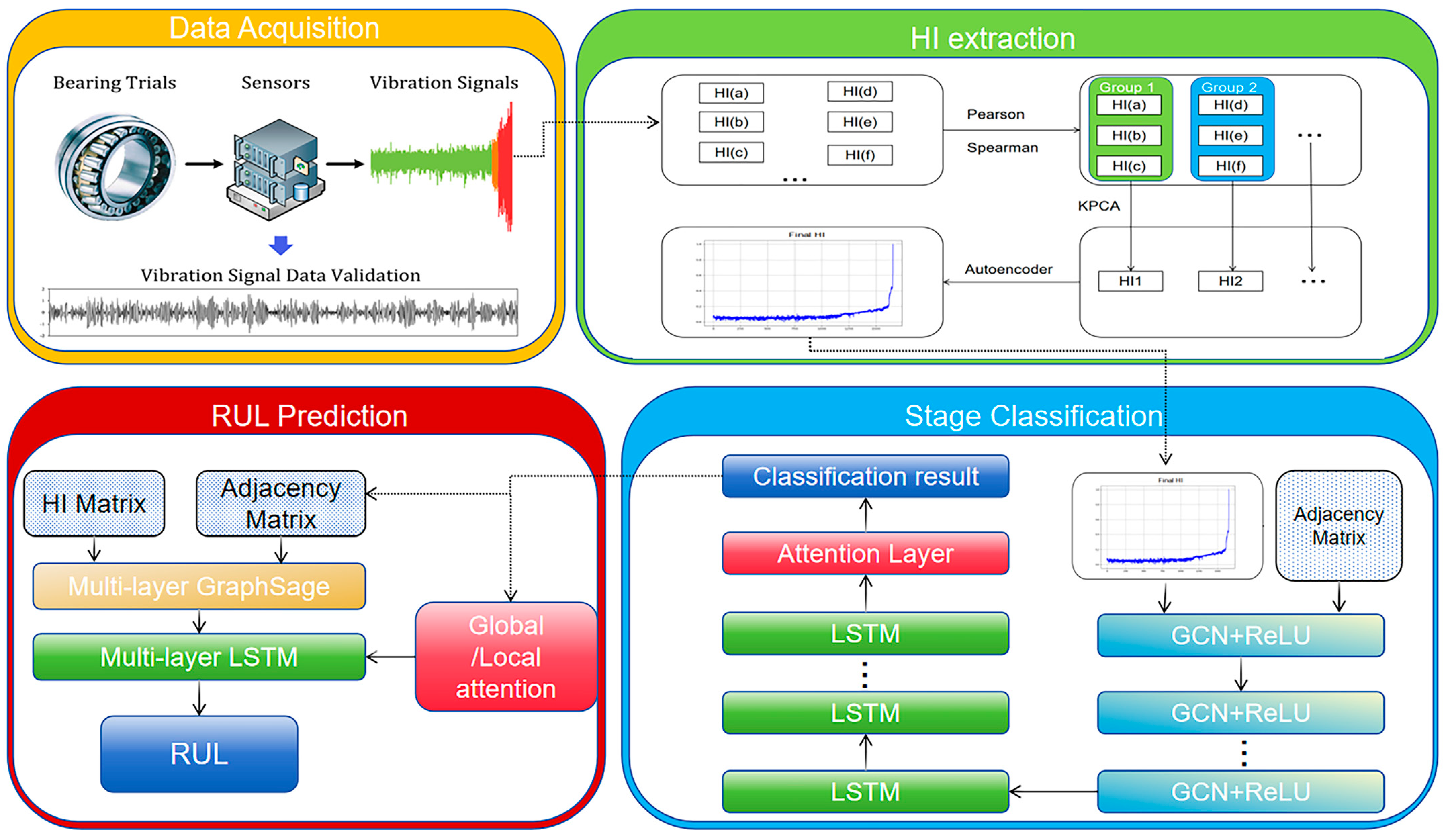
2. Methodology
2.1. Methodological Approach to HI Extraction
2.1.1. HIs
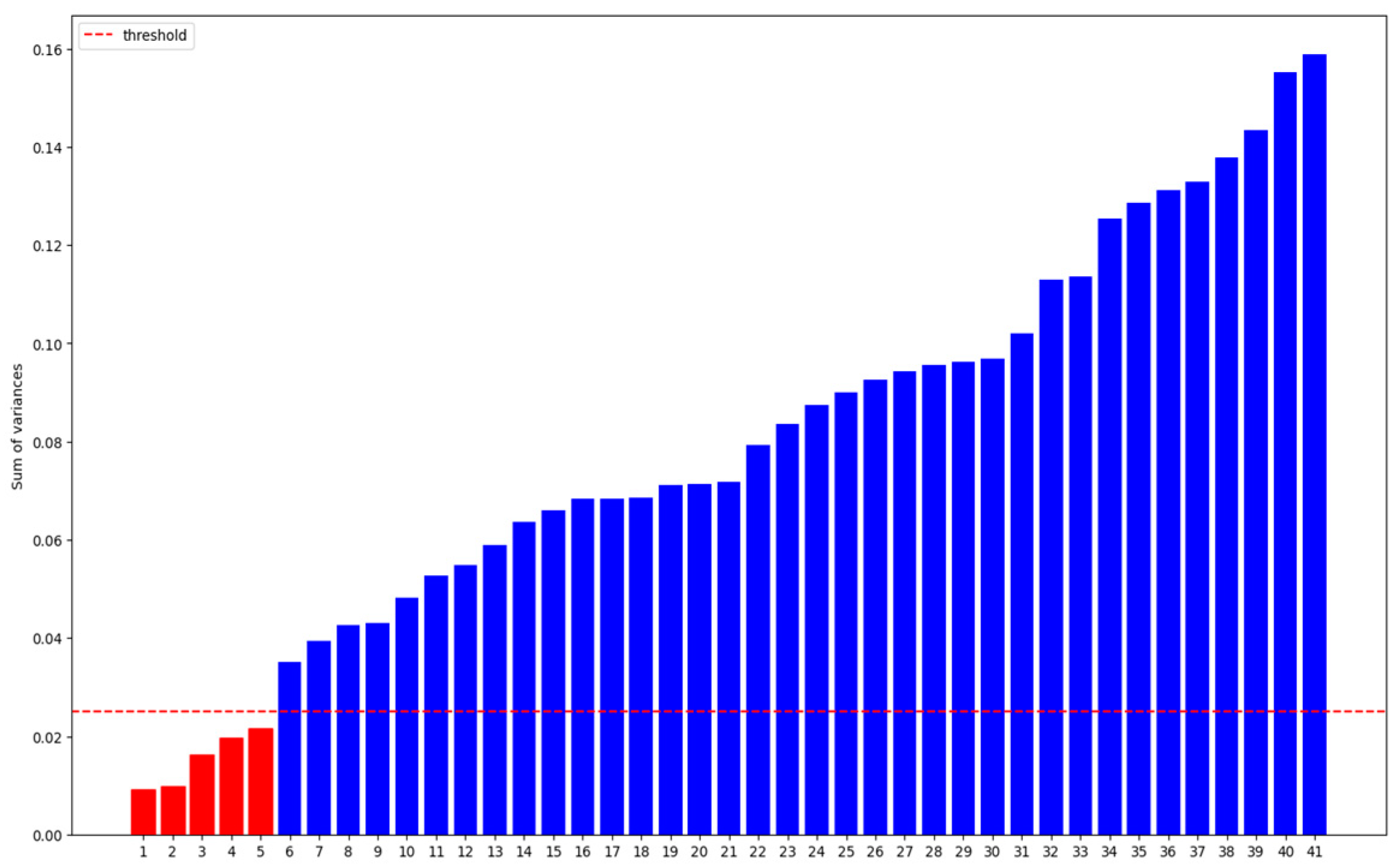
2.1.2. Feature Selection Based on Variance
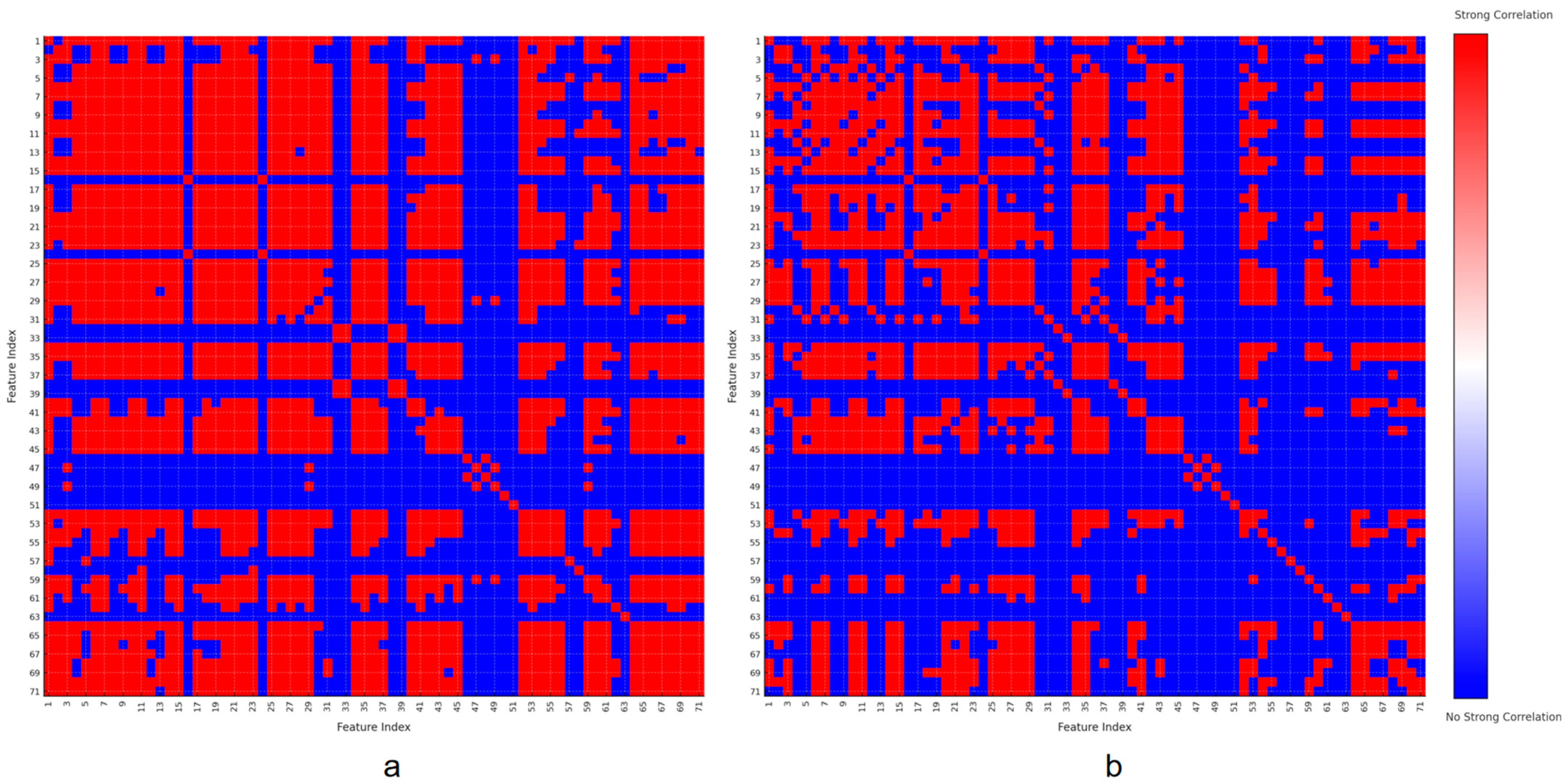
2.1.3. Pearson–Spearman Correlation Analysis
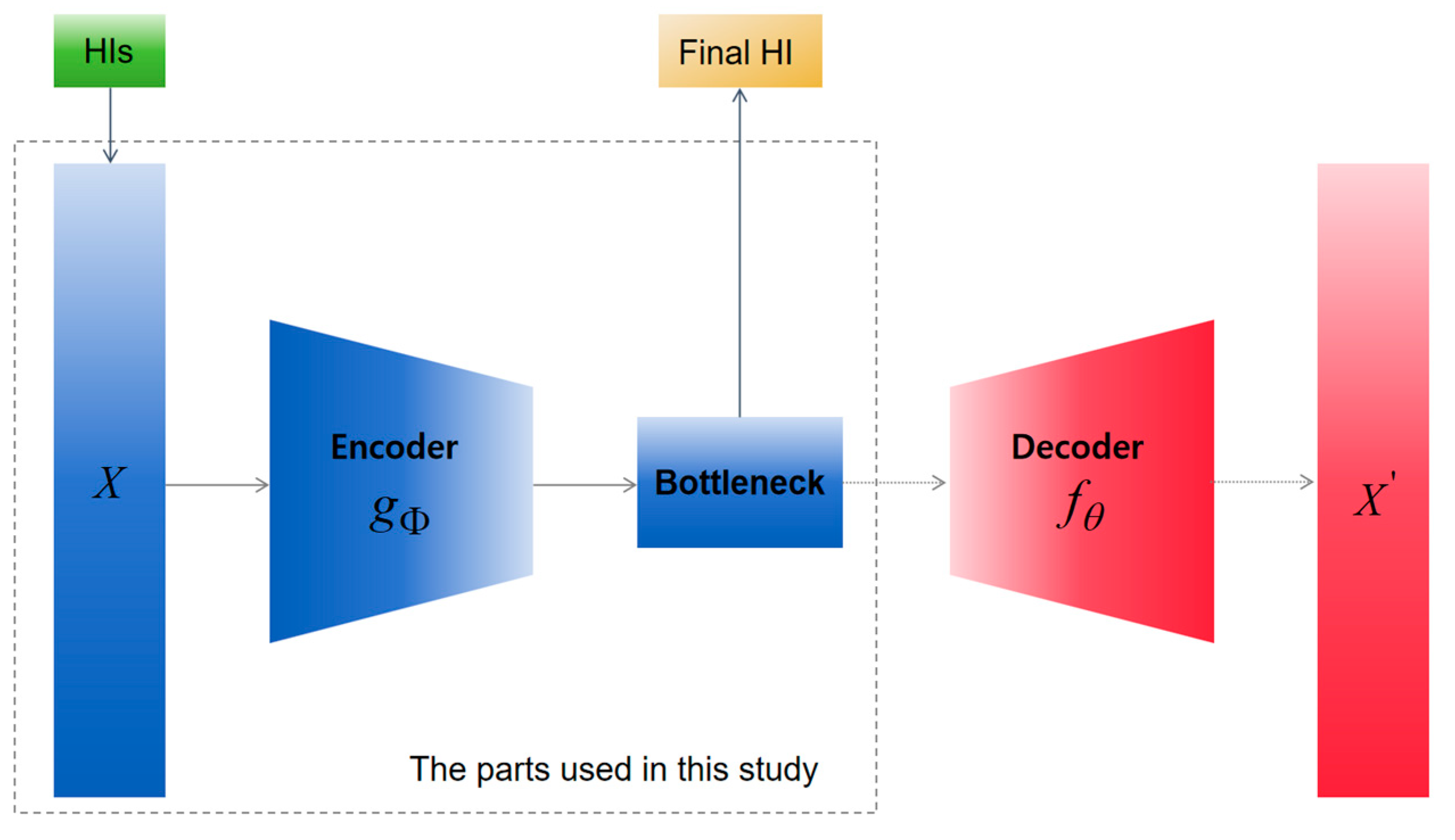
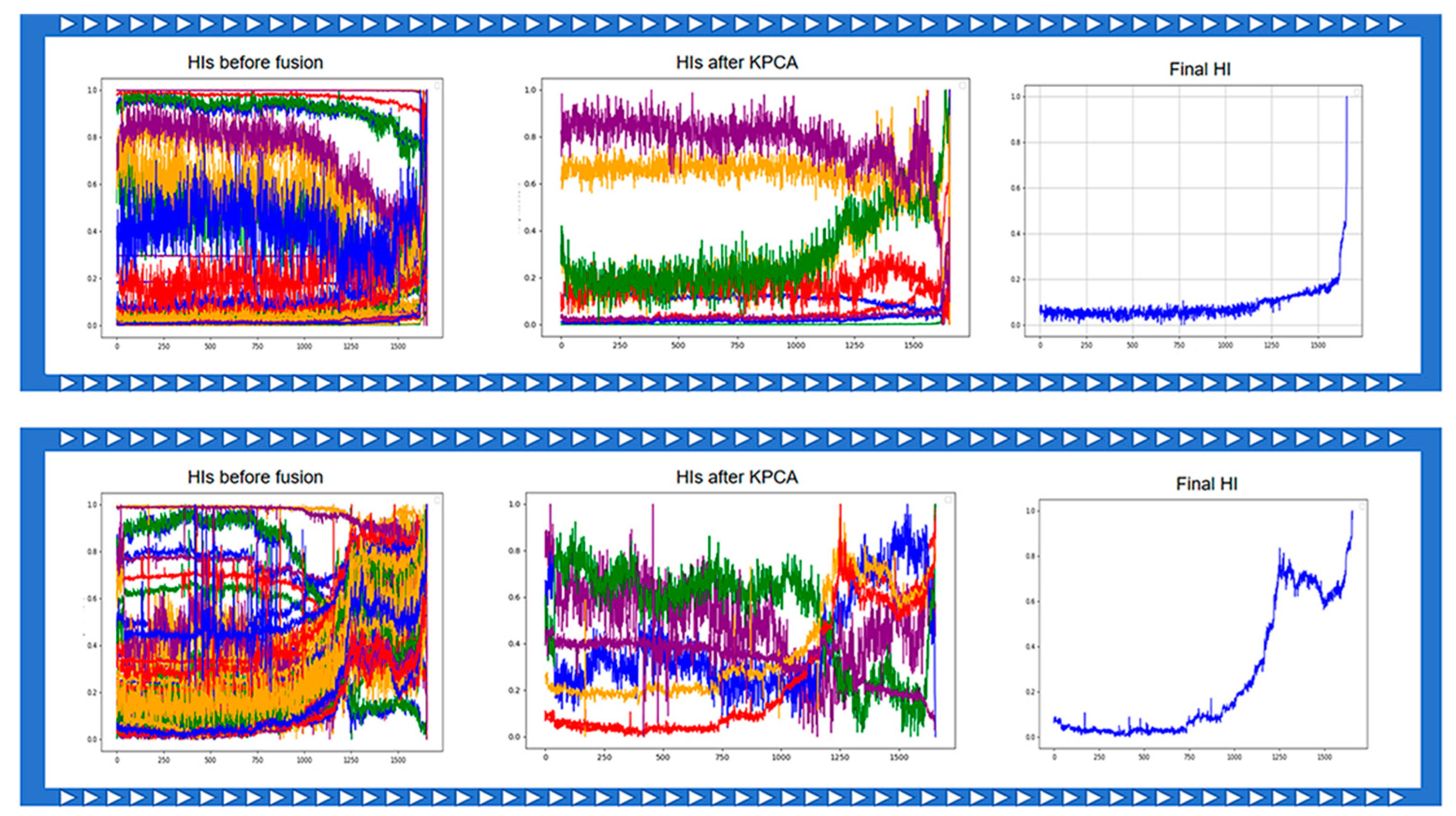
2.1.4. HIs Fusion with KPCA and Autoencoders
- Correlation analysis and grouping: First, perform correlation analysis on the features and set a threshold to group highly correlated features together.
- KPCA processing: Apply KPCA to each group of features, retaining principal components that explain 90% of the cumulative variance.
- Autoencoder optimization: Input the retained principal components and ungrouped features into an autoencoder, adjusting the learning weights according to the original number of features. The output from the bottleneck layer of the autoencoder is used as the final HI, representing the bearing’s degradation state.
2.2. Bearing Degradation Stage Classification
2.2.1. Gaussian Mixture Model (GMM)
- Mean vector :
- Covariance matrix :
- Mixing coefficient :
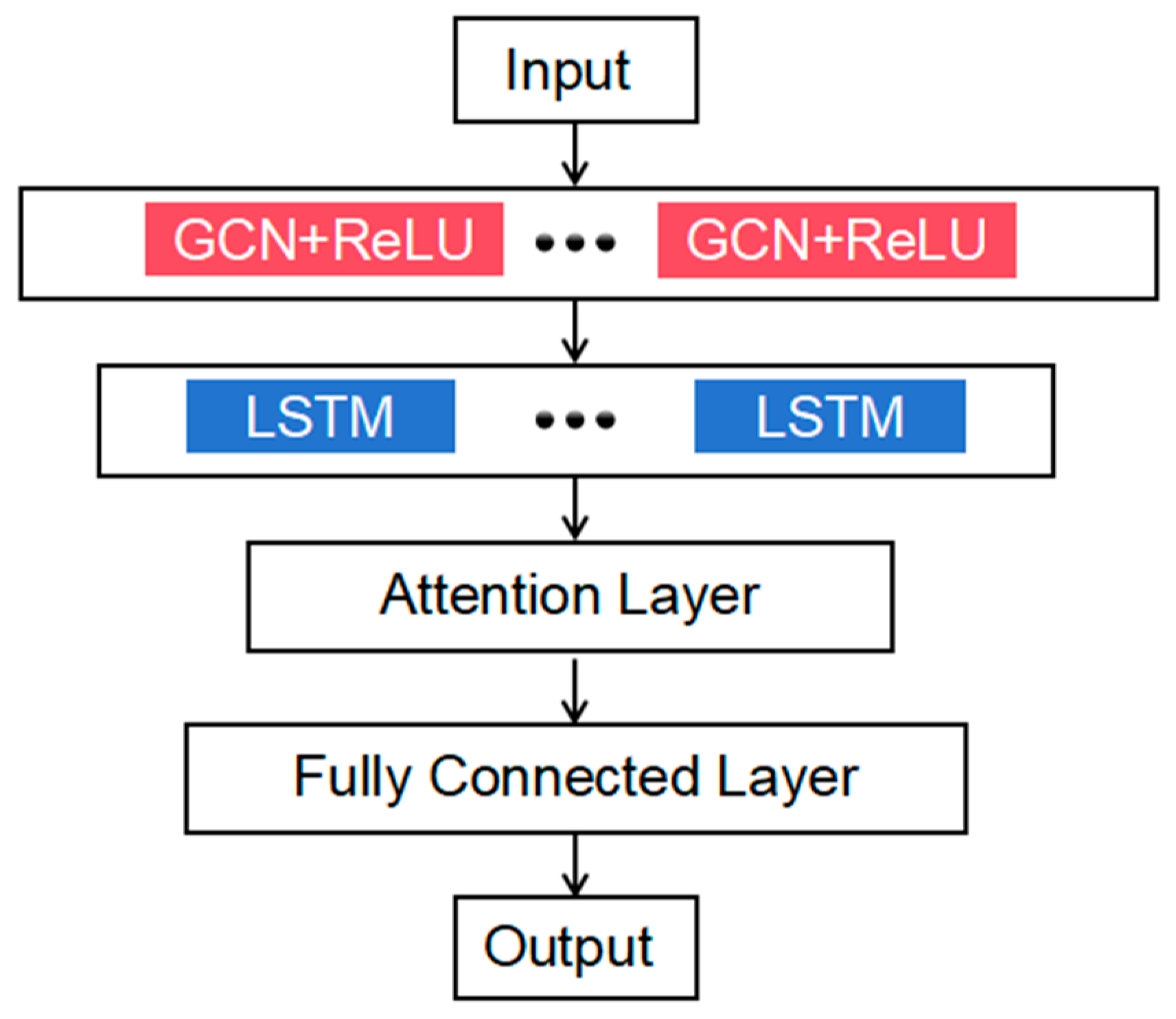
2.2.2. Graph Convolutional Network
2.2.3. GCN–LSTM
- 1.
- Euclidean distance calculation:
- 2.
- Initial connections:
- 3.
- Additional neighbors selection:
- 4.
- Weight distribution:
| Algorithm 1. The pseudocode for constructing the adjacency matrix in the RUL prediction model. |
| Input: Feature matrix X, Node count N, Number of neighbors k, Self-loop weight Ws Output: Adjacency matrix A for i in range(1, N) do: for j in range(1, N) do: if i != j: distance(i, j) = compute_distance(X[i], X[j]); end if end for A[i][i] = Ws; for offset in range(−3, 4): neighbor_idx = (i + offset) % N; if neighbor_idx != i: A[i][neighbor_idx] = 1; end if end for sort distances[i] in ascending order; nearest_neighbors = distances[i][:k]; for neighbor in nearest_neighbors do: A[i][neighbor] = 1/(distance(i, neighbor) + epsilon); end for row_sum = sum(A[i]) − A[i][i]; for j in range(1, N) do: if A[i][j] != 0: A[i][j] = (1 − Ws)*A[i][j]/row_sum; end if end for return A; |
2.3. Bearing Remaining Useful Life Prediction
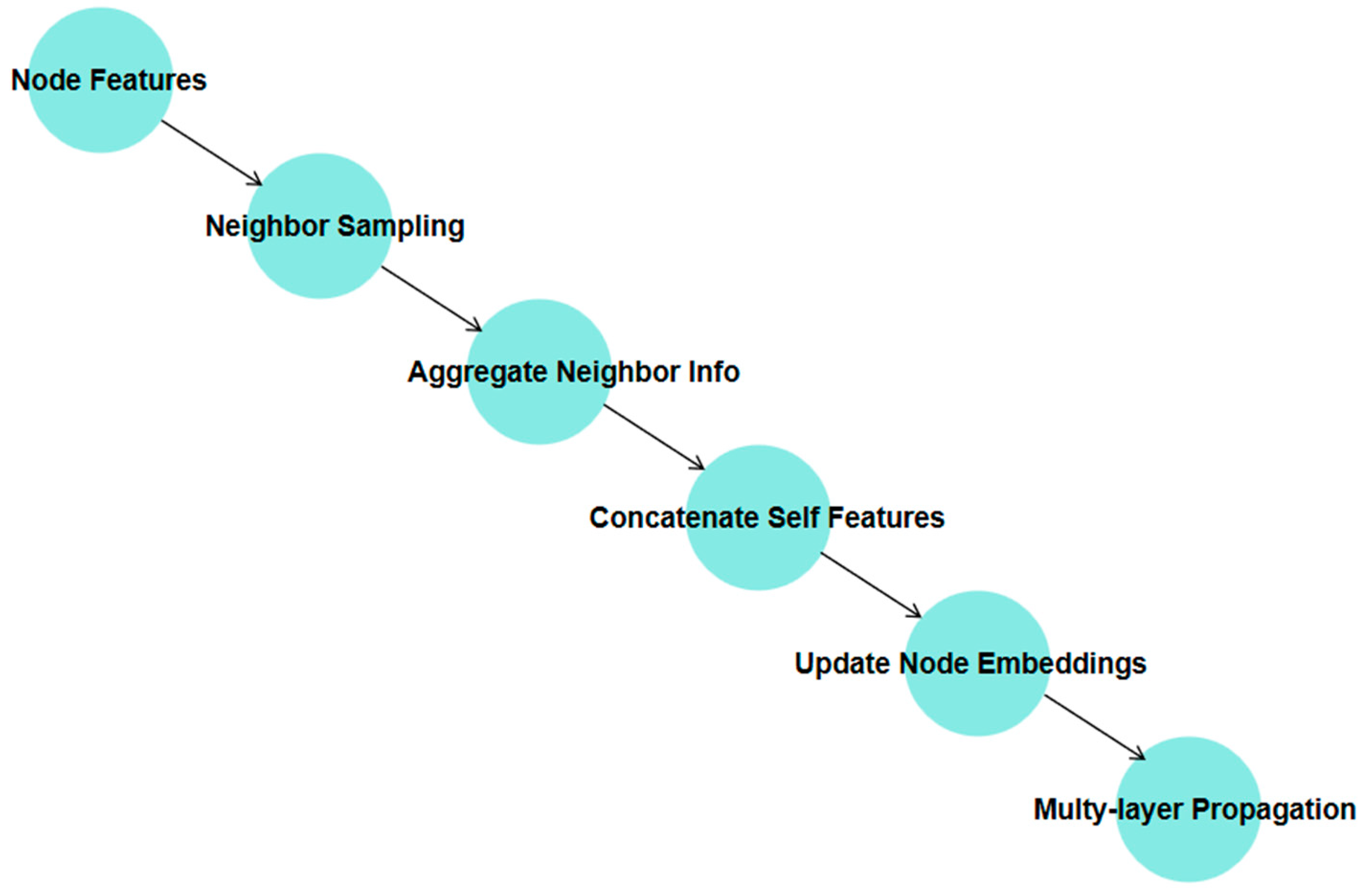
2.3.1. GraphSAGE
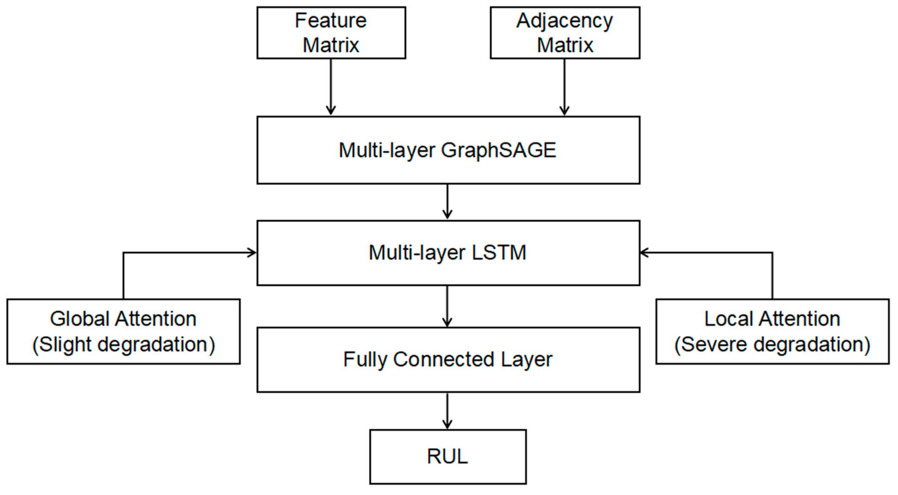
2.3.2. Adaptive Attention GraphSAGE–LSTM
- GraphSAGE feature extractor: First, GraphSAGE is used to extract both local and global spatial features from bearing data. These features reflect the bearing’s state during both healthy and degraded phases, providing input for subsequent time-series modeling. The multi-layer structure of GraphSAGE allows it to iteratively aggregate information from neighboring nodes, capturing high-order dependencies. This is especially well-suited for bearing degradation data with complex topologies.
- LSTM temporal dynamics modeling: The extracted spatial features are fed into an LSTM network to capture the temporal dynamics of the bearing degradation process. LSTM effectively models long-term dependencies over time, helping to identify trends and changes across different degradation phases. Given that degradation process features often exhibit significant temporal dependencies, LSTM’s memory mechanism is well-equipped to model these, providing more accurate predictions of degradation states.
- Adaptive attention mechanism: The model incorporates different attention mechanisms at various stages of degradation to better capture critical features. In the early stages of degradation, where it is important to detect overall trends, the model uses a global attention mechanism to identify key features across the entire sequence, aiding in the early detection of degradation trends. In the severe degradation stage, where short-term features become more significant, the model applies a local attention mechanism to focus on rapid changes over short periods, providing a more detailed description of severe degradation.
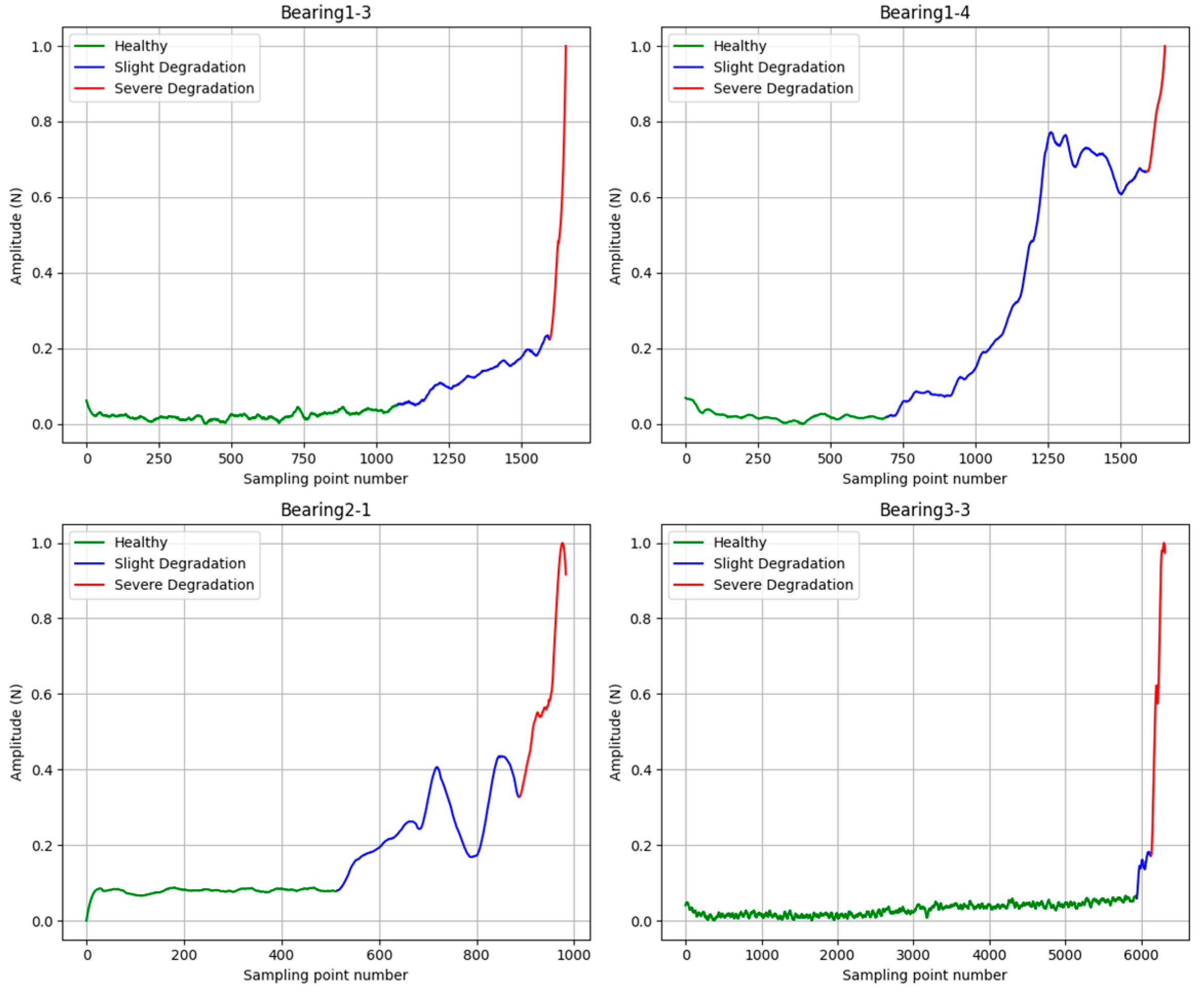
- Healthy stage: Since feature changes are minimal, the adjacency matrix construction remains simple. Each node is connected to itself, as well as to its preceding and following neighbors, with the weights evenly distributed (each edge weight set to 0.33). This ensures basic connectivity while avoiding overfitting by irrelevant information.
- Slight degradation stage: As feature changes begin to manifest, each node is connected to the two preceding and two following neighbors, as well as to the two other nodes with the smallest Euclidean distances. This results in a total of seven connected nodes, including itself. The self-loop weight is set to 0.1, while the weights for the other connections are assigned based on the inverse of the Euclidean distances, as described in Equations (12) and (13), ensuring that more similar nodes receive higher weights.
- Severe degradation stage: As feature changes become more pronounced, each node is connected to the two preceding and two following neighbors, along with the four other nodes with the smallest Euclidean distances. This forms connections to a total of nine nodes, including itself. The self-loop weight remains at 0.1, and the weights for the other nodes are distributed according to the inverse of the Euclidean distances, as described in Equations (12) and (13).
| Algorithm 2. The pseudocode for constructing the adjacency matrix in the RUL prediction model. |
| Input: Feature matrix X, Node count N, Stage type (Healthy, Slight Degradation, Severe Degradation), Self-loop weight Ws Output: Adjacency matrix A for i in range(1, N) do: for j in range(1, N) do: if i != j: distance(i, j) = compute_distance(X[i], X[j]); end if end for if stage_type == “Healthy”: A[i][i] = Ws; for offset in range(−1, 2): neighbor_idx = (i + offset) % N; if neighbor_idx != i: A[i][neighbor_idx] = 0.33; end if end for else if stage_type == “Slight Degradation”: A[i][i] = Ws; for offset in range(−2, 3): neighbor_idx = (i + offset) % N; if neighbor_idx != i: A[i][neighbor_idx] = 1; end if end for sort distances[i] in ascending order; nearest_neighbors = distances[i][:2]; for neighbor in nearest_neighbors do: A[i][neighbor] = 1/(distance(i, neighbor) + epsilon); end for else if stage_type == “Severe Degradation”: A[i][i] = Ws; for offset in range(−2, 3): neighbor_idx = (i + offset) % N; if neighbor_idx != i: A[i][neighbor_idx] = 1; end if end for sort distances[i] in ascending order; nearest_neighbors = distances[i][:4]; for neighbor in nearest_neighbors do: A[i][neighbor] = 1/(distance(i, neighbor) + epsilon); end for end if if stage_type != “Healthy”: row_sum = sum(A[i]) − A[i][i]; for j in range(1, N) do: if A[i][j] != 0: A[i][j] = (1 − Ws)*A[i][j]/row_sum; end if end for end if end for return A; |
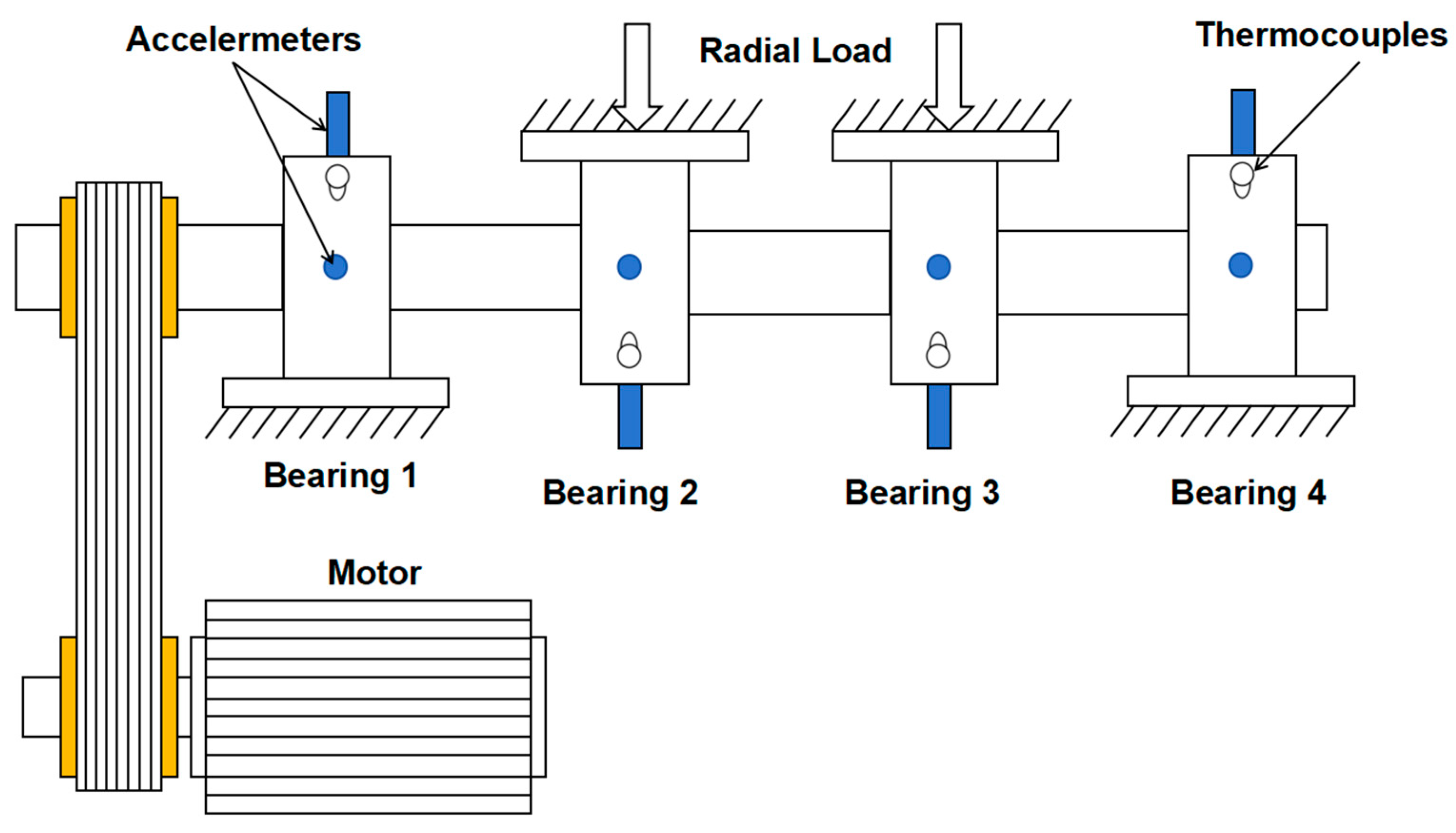
3. Experimental Results
3.1. HI Extraction
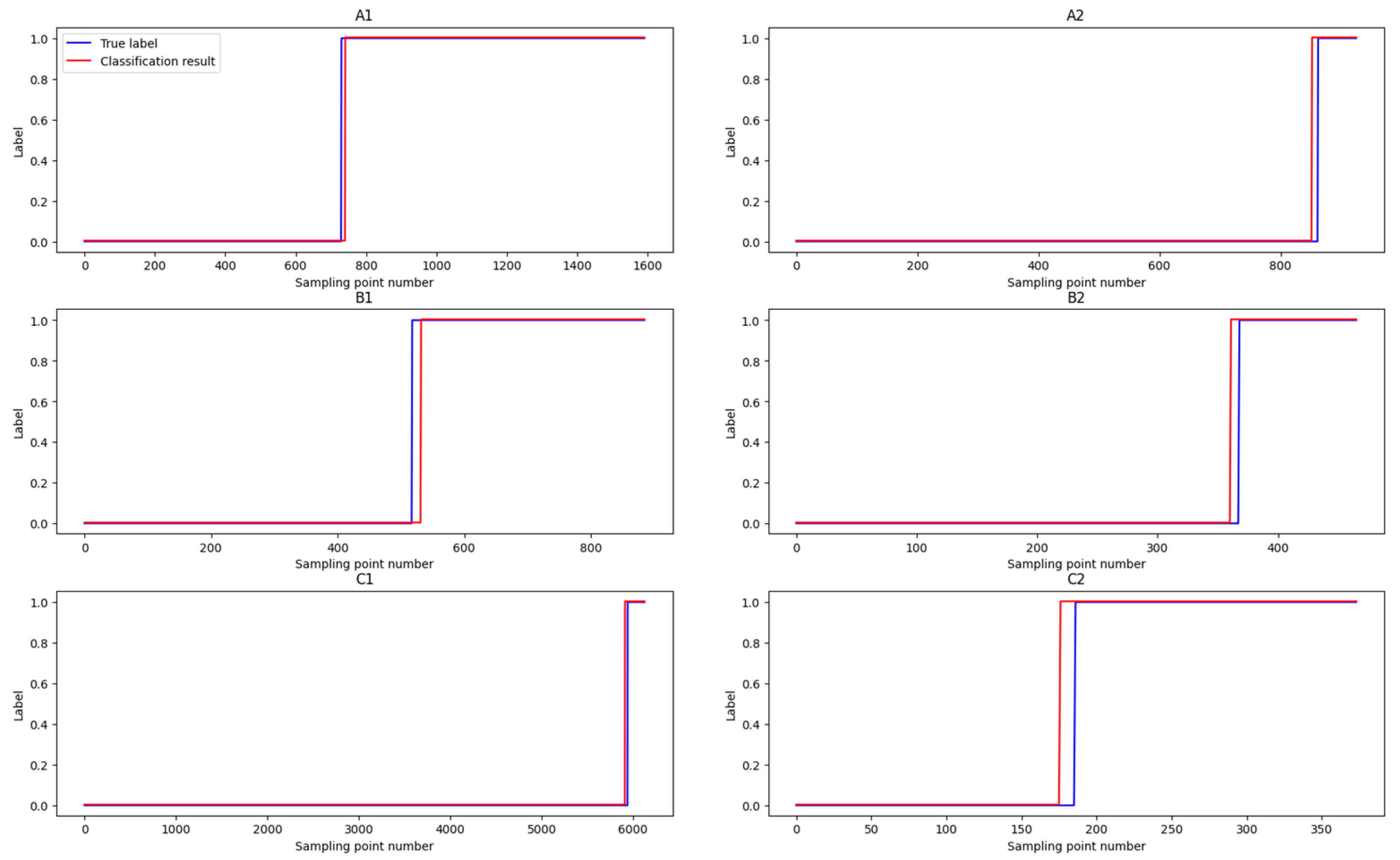
3.2. Stage Classification
- Healthy stage vs. slight degradation stage classification network: This network is used to distinguish between the healthy stage and the slight degradation stage of bearings.
- Slight degradation stage vs. severe degradation stage classification network: This network is used to differentiate between the slight degradation and severe degradation stages.
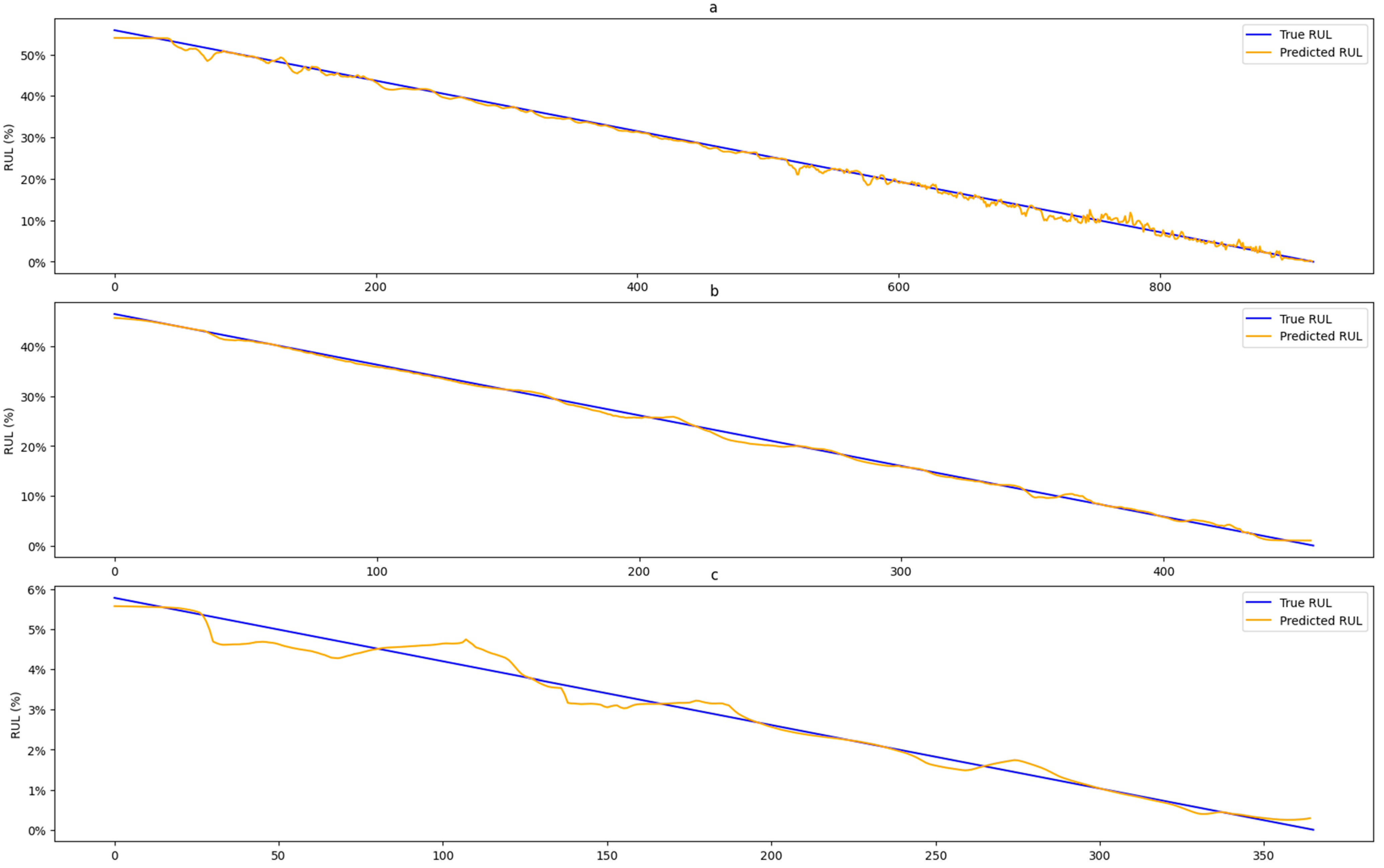
3.3. RUL Prediction
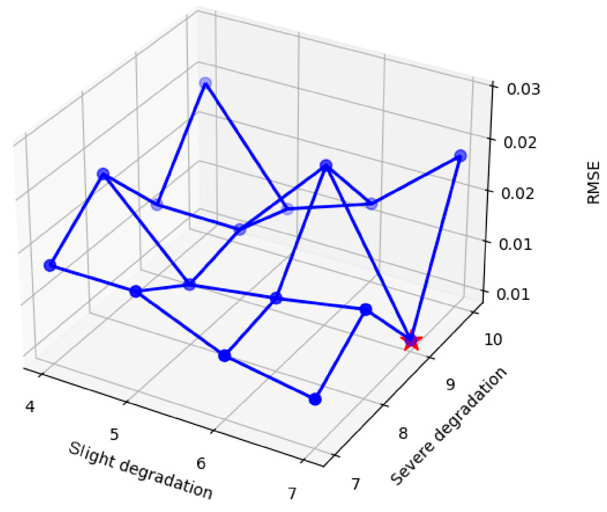
3.4. Parameter Analysis
4. Discussion
Author Contributions
Funding
Data Availability Statement
Conflicts of Interest
References
- Du, X.; Jia, W.; Yu, P.; Shi, Y.; Gong, B. RUL prediction based on GAM–CNN for rotating machinery. J. Braz. Soc. Mech. Sci. Eng. 2023, 45, 142. [Google Scholar] [CrossRef]
- Lei, Y.; Li, N.; Guo, L.; Li, N.; Yan, T.; Lin, J. Machinery health prognostics: A systematic review from data acquisition to RUL prediction. Mech. Syst. Signal Process. 2018, 104, 799–834. [Google Scholar] [CrossRef]
- Pan, C.; Shang, Z.; Liu, F.; Li, W.; Gao, M. Optimization of rolling bearing dynamic model based on improved golden jackal optimization algorithm and sensitive feature fusion. Mech. Syst. Signal Process. 2023, 204, 110845. [Google Scholar] [CrossRef]
- Zhang, Z.X.; Si, X.S.; Hu, C.H. An age-and state-dependent nonlinear prognostic model for degrading systems. IEEE Trans. Reliab. 2015, 64, 1214–1228. [Google Scholar] [CrossRef]
- Gašperin, M.; Juričić, Đ.; Boškoski, P.; Vižintin, J. Model-based prognostics of gear health using stochastic dynamical models. Mech. Syst. Signal Process. 2011, 25, 537–548. [Google Scholar] [CrossRef]
- Soualhi, A.; Medjaher, K.; Zerhouni, N. Bearing health monitoring based on Hilbert–Huang transform, support vector machine, and regression. IEEE Trans. Instrum. Meas. 2014, 64, 52–62. [Google Scholar] [CrossRef]
- Tayade, A.; Patil, S.; Phalle, V.; Kazi, F.; Powar, S. Remaining useful life (RUL) prediction of bearing by using regression model and principal component analysis (PCA) technique. Vibroeng. Procedia 2019, 23, 30–36. [Google Scholar] [CrossRef]
- Li, Z.; Jiang, W.; Zhang, S.; Xue, D.; Zhang, S. Research on prediction method of hydraulic pump remaining useful life based on KPCA and JITL. Appl. Sci. 2021, 11, 9389. [Google Scholar] [CrossRef]
- Zhao, M.; Tang, B.; Tan, Q. Bearing remaining useful life estimation based on time–frequency representation and supervised dimensionality reduction. Measurement 2016, 86, 41–55. [Google Scholar] [CrossRef]
- Dong, S.; Wu, W.; He, K.; Mou, X. Rolling bearing performance degradation assessment based on improved convolutional neural network with anti-interference. Measurement 2020, 151, 107219. [Google Scholar] [CrossRef]
- Yang, D.; Lv, Y.; Yuan, R.; Yang, K.; Zhong, H. A novel vibro-acoustic fault diagnosis method of rolling bearings via entropy-weighted nuisance attribute projection and orthogonal locality preserving projections under various operating conditions. Appl. Acoust. 2022, 196, 108889. [Google Scholar] [CrossRef]
- Akpudo, U.E.; Hur, J.W. A feature fusion-based prognostics approach for rolling element bearings. J. Mech. Sci. Technol. 2020, 34, 4025–4035. [Google Scholar] [CrossRef]
- Wang, Y.; Zhao, J.; Yang, C.; Xu, D.; Ge, J. Remaining useful life prediction of rolling bearings based on Pearson correlation-KPCA multi-feature fusion. Measurement 2022, 201, 111572. [Google Scholar] [CrossRef]
- Wang, Y.; Peng, Y.; Zi, Y.; Jin, X.; Tsui, K.-L. A two-stage data-driven-based prognostic approach for bearing degradation problem. IEEE Trans. Ind. Inform. 2016, 12, 924–932. [Google Scholar] [CrossRef]
- Ni, Q.; Ji, J.C.; Feng, K. Data-driven prognostic scheme for bearings based on a novel health indicator and gated recurrent unit network. IEEE Trans. Ind. Inform. 2022, 19, 1301–1311. [Google Scholar] [CrossRef]
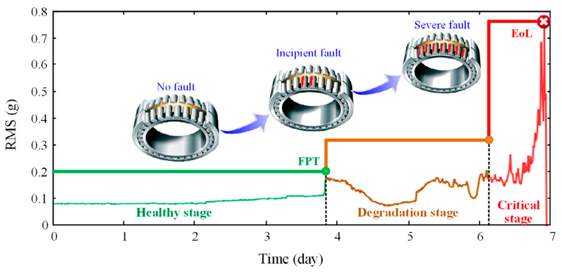
- El-Thalji, I.; Jantunen, E. A descriptive model of wear evolution in rolling bearings. Eng. Fail. Anal. 2014, 45, 204–224. [Google Scholar] [CrossRef]
- Zhao, H.; Liu, H.; Jin, Y.; Dang, X.; Deng, W. Feature extraction for data-driven remaining useful life prediction of rolling bearings. IEEE Trans. Instrum. Meas. 2021, 70, 1–10. [Google Scholar] [CrossRef]
- Ben Ali, J.; Chebel-Morello, B.; Saidi, L.; Malinowski, S.; Fnaiech, F. Accurate bearing remaining useful life prediction based on Weibull distribution and artificial neural network. Mech. Syst. Signal Process. 2015, 56, 150–172. [Google Scholar] [CrossRef]
- Wang, Z.; Zhao, W.; Li, Y.; Dong, L.; Wang, J.; Du, W.; Jiang, X. Adaptive staged RUL prediction of rolling bearing. Measurement 2023, 222, 113478. [Google Scholar] [CrossRef]
- Liu, C.; Chen, Y.; Xu, X. Fatigue life prognosis of composite structures using a transferable deep reinforcement learning-based approach. Compos. Struct. 2025, 353, 118727. [Google Scholar] [CrossRef]
- Yang, X.; Zheng, Y.; Zhang, Y.; Wong, D.S.-H.; Yang, W. Bearing remaining useful life prediction based on regression shapalet and graph neural network. IEEE Trans. Instrum. Meas. 2022, 71, 1–12. [Google Scholar] [CrossRef]
- Wen, G.; Lei, Z.; Chen, X.; Huang, X. Remaining Life Assessment of Rolling Bearing Based on Graph Neural Network. In New Generation Artificial Intelligence-Driven Diagnosis and Maintenance Techniques: Advanced Machine Learning Models, Methods and Applications; Springer Nature: Singapore, 2024; pp. 281–298. [Google Scholar]
- Cui, L.; Xiao, Y.; Liu, D.; Han, H. Digital twin-driven graph domain adaptation neural network for remaining useful life prediction of rolling bearing. Reliab. Eng. Syst. Saf. 2024, 245, 109991. [Google Scholar] [CrossRef]
- Yang, X.; Li, X.; Zheng, Y.; Zhang, Y.; Wong, D.S.-H. Bearing remaining useful life prediction using spatial-temporal multiscale graph convolutional neural network. Meas. Sci. Technol. 2023, 34, 085009. [Google Scholar] [CrossRef]
- Ran, B.; Peng, Y.; Wang, Y. Bearing degradation prediction based on deep latent variable state space model with differential transformation. Mech. Syst. Signal Process. 2024, 220, 111636. [Google Scholar] [CrossRef]
- Cho, I.; Park, S.; Kim, J. A fire risk assessment method for high-capacity battery packs using interquartile range filter. J. Energy Storage 2022, 50, 104663. [Google Scholar] [CrossRef]
- Sehgal, R.; Jagadesh, P. Data-driven robust portfolio optimization with semi mean absolute deviation via support vector clustering. Expert Syst. Appl. 2023, 224, 120000. [Google Scholar] [CrossRef]
- Vatanshenas, A.; Länsivaara, T.T. Estimating maximum shear modulus (G0) using adaptive neuro-fuzzy inference system (ANFIS). Soil Dyn. Earthq. Eng. 2022, 153, 107105. [Google Scholar] [CrossRef]
- Hou, D.; Chen, J.; Cheng, R.; Hu, X.; Shi, P. A bearing remaining life prediction method under variable operating conditions based on cross-transformer fusioning segmented data cleaning. Reliab. Eng. Syst. Saf. 2024, 245, 110021. [Google Scholar] [CrossRef]
- Zhang, X.; Wan, S.; He, Y.; Wang, X.; Dou, L. Teager energy spectral kurtosis of wavelet packet transform and its application in locating the sound source of fault bearing of belt conveyor. Measurement 2021, 173, 108367. [Google Scholar] [CrossRef]
- Jiang, X.; Shen, C.; Shi, J.; Zhu, Z. Initial center frequency-guided VMD for fault diagnosis of rotating machines. J. Sound Vib. 2018, 435, 36–55. [Google Scholar] [CrossRef]
- Chen, P.; He, A.; Zhang, T.; Dong, X. Weak vibration signal detection based on frequency domain cumulative averaging with DVS system. Opt. Fiber Technol. 2024, 88, 103834. [Google Scholar] [CrossRef]
- Mahapatra, A.G.; Horio, K. Classification of ictal and interictal EEG using RMS frequency, dominant frequency, root mean instantaneous frequency square and their parameters ratio. Biomed. Signal Process. Control 2018, 44, 168–180. [Google Scholar] [CrossRef]
- Hashim, S.; Shakya, P. A spectral kurtosis based blind deconvolution approach for spur gear fault diagnosis. ISA Trans. 2023, 142, 492–500. [Google Scholar] [CrossRef]
- Han, S.; Li, D.; Li, K.; Wu, H.; Gao, Y.; Zhang, Y.; Yuan, R. Analysis and study of transmission line icing based on grey correlation Pearson combinatorial optimization support vector machine. Measurement 2024, 236, 115086. [Google Scholar] [CrossRef]
- Jiang, J.; Zhang, X.; Yuan, Z. Feature selection for classification with Spearman’s rank correlation coefficient-based self-information in divergence-based fuzzy rough sets. Expert Syst. Appl. 2024, 249, 123633. [Google Scholar] [CrossRef]
- Zhang, Z.; Tang, X.; Liu, C.; Li, X.; Ren, S. Multiple ultrasonic partial discharge DOA estimation performance of KPCA Pseudo-Whitening mnc-FastICA. Measurement 2024, 231, 114596. [Google Scholar] [CrossRef]
- Zhang, M.; Zhong, J.; Zhou, C.; Jia, X.; Zhu, X.; Huang, B. Deep learning-driven pavement crack analysis: Autoencoder-enhanced crack feature extraction and structure classification. Eng. Appl. Artif. Intell. 2024, 132, 107949. [Google Scholar] [CrossRef]
- Chaleshtori, A.E.; Aghaie, A. A novel bearing fault diagnosis approach using the Gaussian mixture model and the weighted principal component analysis. Reliab. Eng. Syst. Saf. 2024, 242, 109720. [Google Scholar] [CrossRef]
- Song, L.; Jin, Y.; Lin, T.; Zhao, S.; Wei, Z.; Wang, H. Remaining Useful Life Prediction Method Based on the Spatiotemporal Graph and GCN Nested Parallel Route Model. IEEE Trans. Instrum. Meas. 2024, 73, 1–12. [Google Scholar] [CrossRef]
- Kamat, P.; Kumar, S.; Sugandhi, R. Vibration-based anomaly pattern mining for remaining useful life (RUL) prediction in bearings. J. Braz. Soc. Mech. Sci. Eng. 2024, 46, 290. [Google Scholar] [CrossRef]
- Tao, L.; Wu, H.; Zheng, X. Remaining Useful Life Prediction of Lithium-ion Batteries Based on Multi-graph-network model. In Proceedings of the 2024 43rd Chinese Control Conference (CCC), Kunming, China, 28–31 July 2024; pp. 8477–8482. [Google Scholar]
- Ding, H.; Yang, L.; Cheng, Z.; Yang, Z. A remaining useful life prediction method for bearing based on deep neural networks. Measurement 2021, 172, 108878. [Google Scholar] [CrossRef]
- Yang, C.; Ma, J.; Wang, X.; Li, X.; Li, Z.; Luo, T. A novel based-performance degradation indicator RUL prediction model and its application in rolling bearing. ISA Trans. 2022, 121, 349–364. [Google Scholar] [CrossRef] [PubMed]
- Ding, G.; Wang, W.; Zhao, J. Prediction of remaining useful life of rolling bearing based on fractal dimension and convolutional neural network. Meas. Control 2022, 55, 79–93. [Google Scholar] [CrossRef]


| Feature | Formula | Feature | Formula |
|---|---|---|---|
| Interquartile range | Peak to peak | ||
| Kurtosis | Root mean square | ||
| Kurtosis indicator | Signal entropy | ||
| Waveform indicator | RMSEE | ||
| Margin indicator | Modulus maximum | ||
| Skewness | Teager energy mean | ||
| Peak indicator | Variance | ||
| Pulse indicator | Mean absolute deviation |
| Feature | Formula |
|---|---|
| Center frequency | |
| Frequency domain amplitude average | |
| Root mean square frequency | |
| Standard deviation frequency | |
| Peak frequency | |
| Spectral energy | |
| Spectral entropy | |
| Spectral flatness | |
| Spectral kurtosis | |
| Spectral skewness | |
| Spectral spread |
| Features Before Initial Selection | Features After Initial Selection | ||
|---|---|---|---|
| IQR | FDAA | IQR | Spectral entropy |
| Kurtosis | Peak frequency | Kurtosis | Spectral flatness |
| Kurtosis indicator | RMSF | Kurtosis indicator | Spectral kurtosis |
| MAD | Spectral energy | MAD | Spectral skewness |
| Margin indicator | Spectral entropy | Margin indicator | Spectral spread |
| LSS | Spectral flatness | Modulus max | SDF |
| Mean | Spectral kurtosis | Peak indicator | EMD1 |
| Mean square value | Spectral skewness | Peak to peak | EMD2 |
| Median | Spectral spread | Pulse indicator | EMD3 |
| Modulus max | SDF | RMSEE | EMD4 |
| Peak indicator | EMD1 | Root mean square | EMD5 |
| Peak to peak | EMD2 | Signal entropy | WPE2 |
| Pulse indicator | EMD3 | Skewness | WPE3 |
| RMSEE | EMD4 | Teager energy mean | WPE4 |
| Root mean square | EMD5 | Variance | WPE5 |
| Signal entropy | WPE1 | Waveform indicator | |
| Skewness | WPE2 | Center frequency | |
| Teager energy mean | WPE3 | FDAA | |
| Variance | WPE4 | Peak frequency | |
| Waveform indicator | WPE5 | RMSF | |
| Center frequency | Spectral energy | ||
| Group1 | Group2 | Group3 | Group4 |
|---|---|---|---|
| 1, 2, 3, 4, 5, 6, 7, 8, 9, 10, 11, 12, 13, 14, 15, 16, 18, 19, 20, 21, 22, 23, 24, 26, 27, 28, 29, 30, 31, 32, 35, 36, 37, 38, 41, 42, 43, 44, 45, 46, 48, 50, 53, 54, 55, 56, 57, 58, 59, 60, 61, 62, 63, 65, 66, 67, 68, 69, 70, 71, 72 | 33, 34, 39, 40 | 17, 25 | 47, 49 |
| Group1 | Group2 |
|---|---|
| 1, 2, 3, 4, 5, 6, 7, 8, 9, 10, 11, 12, 13, 14, 15, 16, 17, 18, 19, 20, 21, 22, 23, 24, 25, 26, 27, 28, 29, 30, 31, 32, 35, 36, 37, 40, 41, 42, 43, 44, 45, 46, 51, 52, 53, 54, 55, 56, 57, 58, 59, 60, 61, 62, 63, 64, 65, 66, 67, 68, 69, 70, 71, 72 | 33, 34, 38, 39 |
| Parameters | Parameter Value | Parameters | Parameter Value |
|---|---|---|---|
| GCN layers | 3 | Activation function | ReLU |
| GCN channels | 32 | Optimizer | NAdam |
| LSTM layers | 6 | Learning rate | 0.0001 |
| LSTM hidden layers | 64 | Loss function | CrossEntropyLoss |
| Parameters | Parameter Value | Parameters | Parameter Value |
|---|---|---|---|
| GCN layers | 3 | Activation function | ReLU |
| GCN channels | 64 | Optimizer | NAdam |
| LSTM layers | 8 | Learning rate | 0.00015 |
| LSTM hidden layers | 64 | Loss function | CrossEntropyLoss |
| Models | Bearing 1-4 | Bearing 2-1 | Bearing 3-3 |
|---|---|---|---|
| GCN–LSTM | 99.31%/98.92% | 98.42%/98.50% | 99.53%/97.33% |
| CNN | 82.27%/76.13% | 79.81%/80.29% | 72.45%/69.88% |
| GCN | 88.40%/83.44% | 84.62%/82.46% | 86.91%/87.69% |
| CCN–LSTM | 94.57%96.83% | 89.45%/90.68% | 93.40%/94.74% |
| Bearings | RMSE | MAE | MAPE | R2 | Adjusted R2 |
|---|---|---|---|---|---|
| Bearing 1-4 | 0.00706 | 0.00599 | 0.04994 | 0.997555 | 0.997552 |
| Bearing 2-1 | 0.00494 | 0.00403 | 0.07415 | 0.998545 | 0.998542 |
| Bearing 3-3 | 0.00265 | 0.00180 | 0.17506 | 0.978568 | 0.978509 |
| Models | 1-4 | 2-1 | 3-3 |
|---|---|---|---|
| AAGL | 0.00706 | 0.00494 | 0.00265 |
| [43] | 0.00772 | 0.00525 | 0.00732 |
| [44] | 0.1739 | - | - |
| [45] | 0.0691 | 0.1071 | 0.0822 |
| Models | 1-4 | 2-1 | 3-3 |
|---|---|---|---|
| LSTM | 0.02732 | 0.01492 | 0.02346 |
| CNN–LSTM | 0.01613 | 0.00963 | 0.01372 |
| GCN–LSTM | 0.00967 | 0.007670 | 0.00663 |
| AAGL | 0.00706 | 0.00494 | 0.00265 |
Disclaimer/Publisher’s Note: The statements, opinions and data contained in all publications are solely those of the individual author(s) and contributor(s) and not of MDPI and/or the editor(s). MDPI and/or the editor(s) disclaim responsibility for any injury to people or property resulting from any ideas, methods, instructions or products referred to in the content. |
© 2025 by the authors. Licensee MDPI, Basel, Switzerland. This article is an open access article distributed under the terms and conditions of the Creative Commons Attribution (CC BY) license (https://creativecommons.org/licenses/by/4.0/).
Share and Cite
Huang, G.; Lei, W.; Dong, X.; Zou, D.; Chen, S.; Dong, X. Stage-Based Remaining Useful Life Prediction for Bearings Using GNN and Correlation-Driven Feature Extraction. Machines 2025, 13, 43. https://doi.org/10.3390/machines13010043
Huang G, Lei W, Dong X, Zou D, Chen S, Dong X. Stage-Based Remaining Useful Life Prediction for Bearings Using GNN and Correlation-Driven Feature Extraction. Machines. 2025; 13(1):43. https://doi.org/10.3390/machines13010043
Chicago/Turabian StyleHuang, Guangzhong, Wenping Lei, Xinmin Dong, Dongliang Zou, Shijin Chen, and Xing Dong. 2025. "Stage-Based Remaining Useful Life Prediction for Bearings Using GNN and Correlation-Driven Feature Extraction" Machines 13, no. 1: 43. https://doi.org/10.3390/machines13010043
APA StyleHuang, G., Lei, W., Dong, X., Zou, D., Chen, S., & Dong, X. (2025). Stage-Based Remaining Useful Life Prediction for Bearings Using GNN and Correlation-Driven Feature Extraction. Machines, 13(1), 43. https://doi.org/10.3390/machines13010043