Analyzing Higher-Order Curvature of Four-Bar Linkages with Derivatives of Screws

Abstract

Curvature theory, a fundamental subject in kinematics, is typically addressed through the concepts of instantaneous invariants and canonical coordinates, which are pivotal for the generation of mechanical paths. This paper delves into this subject with a higher-order analysis of screws, employing both canonical and natural coordinates. Through this exploration, a new Euler–Savary equation is derived, one that does not rely on canonical coordinates. Additionally, the paper provides a comprehensive classification of the degenerate conditions of the cubic of stationary curves of four-bar linkages at rotational positions. A thorough examination of four-bar linkages in translational positions—the couple links translate instantaneously—is also presented, with analyses extending up to the sixth order. The findings reveal that the Burmester’s points at translational positions can be extended to Burmester’s points with excess one, provided that all pivot points are symmetrically distributed about the pole norm with the two cranks in corotating senses. However, the extension to Burmester’s points with excess two is not possible. Similarly, the Ball’s point with excess one does not progress to Ball’s point with excess two. The paper also highlights that the traditional method, which is based on canonical coordinates, is ineffective when the four-bar linkage forms a parallelogram. Fortunately, this scenario can be effectively analyzed using the screw-based approach. Ultimately, the results presented can also serve as analytical solutions for 3-RR platforms with higher-order shakiness.

1. Introduction

Curvature theory of path-curves is a classic topic in theoretical kinematics [1,2,3,4,5,6] and plays a key role in the mechanical generation of curves [7,8,9,10,11], such as straight-line, circular-arc, and other more general curves for planar mechanisms [12,13] and spherical mechanisms [14,15]. Traditionally, curvature theory was mainly studied based on the concept of instantaneous invariants and canonical coordinate systems [1,2]. The concept of instantaneous invariants, which are the geometric properties of a rigid-body motion, was introduced by Bottema and Veldkamp [7]. A canonical coordinate system is a special frame in which the kinematics can be formed with a minimum number of coordinates. Veldkamp has made an extensive study on the curvature of plane algebraic curves, and applied it to four-bar linkages [2,3]. However, for the four-bar in a translational position instantaneously, he did not give a clear condition for the Burmester’s point with excess one, as well as the Ball’s points with excess, and whether they are the highest order, which is important for the design of Watt mechanisms [16]. The degenerate conditions for the cubic of stationary curvature have been discussed in detail in the publications by Veldkamp [2] and Dijksman [6], but a clear and concise algebraic classification that relates to the geometry of four-bars has been not reported.

In mechanism theory, curvature theory is in fact involved in the singularity problems [17,18]. For example, if we attach a third link to the four-bar linkage and its link axis also intersects at the velocity pole of the original four-bar linkage, we can obtain a 3-RR linkage (also called a planar platform) with instantaneous mobility (also called shakiness [19,20,21]), which is a structure called an infinitesimal mechanism. The order of mobility of 3-RR linkages is clearly related to the property of the trajectory of the path generated by the original four-bar linkages. If the fixed pivot point of the third link is located at the curvature (first or second derivative of the curvature) center of the moving pivot, the corresponding 3-RR linkages possess second-order (third or fourth order) mobility. In addition, if the fixed pivot point of the third link is located at center of the first or second curvature, the corresponding linkages possess even higher-order mobility; the former corresponds to cubic stationary curvature, the latter to the Burmester’s points, and the resulting 3-RR linkages become highly flexible, although still remaining a structure.

The problem of singularity and higher-order mobility are usually treated with higher-order kinematic analysis of screws, which is a pure algebraic method [22]. Screw theory has been widely used in kinematics and mechanism theory [23,24]. Higher-order analysis of screws has been formulated to an arbitrary order for platform mechanisms by Wohlhart [20,21]. He also pointed out the relationship between the order of shakiness and the order curvature of the trajectory of four-bar linkages. However, he did not give analytical solutions for these shaky structures, even for lower-order shakiness. Possible reasons are that he used a more general reference coordinate system rather than the canonical systems, which make the symbolic computation much more complicated.

Although the classic method based on instantaneous invariants and canonical coordinates is recognized as an elegant way to treat curvature theory, conditions in which the classic methods fail indeed exist, such as the parallelogram, in which the canonical coordinates will approximate to infinity. In addition, it will be shown that a new version of the Euler–Savary equation can be formed neatly without referring to the canonical coordinates. To this end, we revisit the curvature theory of four-bar linkages with screw theory using both canonical coordinates and natural coordinates (selected for convenience). An imaginary link is attached to the four-bar linkages, thus forming a 3-RR platform; thus, Wohlhart’s method can be used for higher-order analysis.

In the following sections, analysis will be performed up to the third order for the four-bar linkages at rotational positions to obtain analytical solutions for curvature and stationary curvature. Analysis will be performed up to the sixth order for the four-bar linkages at translational positions (the couple link translates instantaneously) to analyze the highest-order curvature.

2. Methods

2.1. Higher-Order Kinematics of Platform Mechanisms in Screws

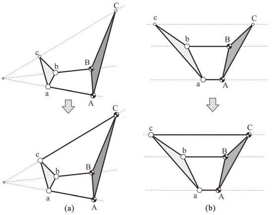
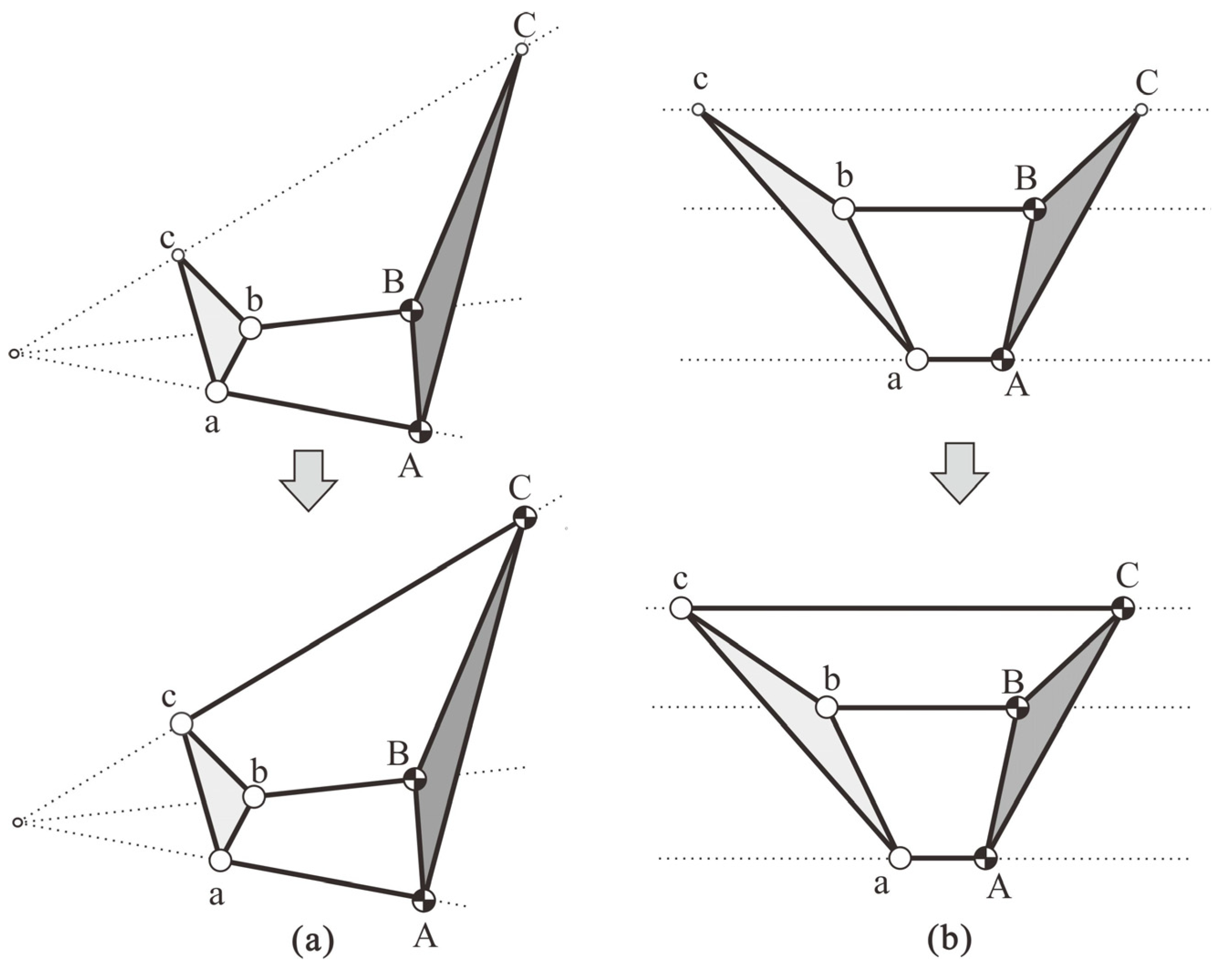
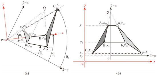
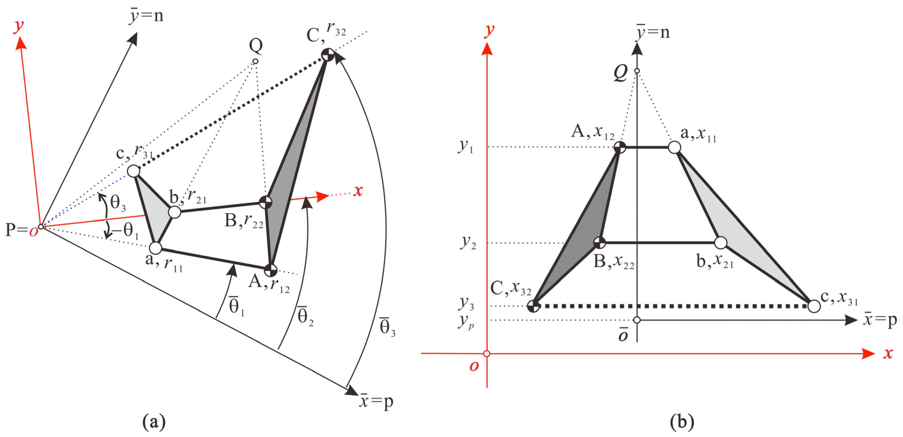
In this paper, a third link is attached to a four-bar linkage, thus forming a 3-RR linkage or a planar Stewart platform, as shown in Figure 1. All the link axes are required to intersect at one point (possibly at infinity). A platform mechanism consists of two rigid bodies, the fixed body and moving body. The two bodies are actuated by linear actuators which are connected by spherical joints for spatial platforms and revolute joints for planar platforms. Generally, there are two situations: the first situation consists of four-bar linkages with a finite pole, and is said to be at rotational position; the second one corresponds to a pole at infinity, and is said to be at translational position, as shown in Figure 1.

Figure 1. Four-bar linkages and the derived planar 3-RR platform, at (a) rotational and (b) translational positions.

The constraints provided by each limb are simply line vectors if the linear actuators are locked. Higher-order constraints of parallel mechanisms can be formulated explicitly to arbitrary order [20,21]. Since analyses up to the sixth order are needed in the following sections, the expressions up to the sixth order are summarized in the following. Denote $\mathit{V}$ as the velocity screw of the moving platform:

$$\mathit{V}=\left(\begin{array}{c}\mathit{\omega }\\ {\mathit{\upsilon }}_0\end{array}\right),$$

(1)

in which $\mathit{\omega }$ is the angular velocity and ${\mathit{\upsilon }}_0$ is the velocity of the point instantaneously coincident with the origin. The higher-order time derivatives of the velocity of the screw up to the fifth order are

$$\dot{\mathit{V}}=\left(\begin{array}{c}\dot{\mathit{\omega }}\\ {\dot{\mathit{\upsilon }}}_0+{\mathit{\upsilon }}_0\times \mathit{\omega }\end{array}\right),$$

(2)

$$\ddot{\mathit{V}}=\left(\begin{array}{c}\ddot{\mathit{\omega }}\\ {\ddot{\mathit{\upsilon }}}_0+{\dot{\mathit{\upsilon }}}_0\times \mathit{\omega }+2{\mathit{\upsilon }}_0\times \dot{\mathit{\omega }}\end{array}\right),$$

(3)

$$\stackrel{⃛}{\mathit{V}}=\left(\begin{array}{c}\stackrel{⃛}{\mathit{\omega }}\\ {\stackrel{⃛}{\mathit{\upsilon }}}_0+{\ddot{\mathit{\upsilon }}}_0\times \mathit{\omega }+3{\dot{\mathit{\upsilon }}}_0\times \dot{\mathit{\omega }}+3{\mathit{\upsilon }}_0\times \ddot{\mathit{\omega }}\end{array}\right),$$

(4)

$${\mathit{V}}^{\left(4\right)}=\left(\begin{array}{c}{\mathit{\omega }}^{\left(4\right)}\\ {\mathit{\upsilon }}_0^{\left(4\right)}+{\stackrel{⃛}{\mathit{\upsilon }}}_0\times \mathit{\omega }+4{\ddot{\mathit{\upsilon }}}_0\times \dot{\mathit{\omega }}+6{\dot{\mathit{\upsilon }}}_0\times \ddot{\mathit{\omega }}+3{\mathit{\upsilon }}_0\times \stackrel{⃛}{\mathit{\omega }}\end{array}\right),$$

(5)

$${\mathit{V}}^{\left(5\right)}=\left(\begin{array}{c}{\mathit{\omega }}^{\left(5\right)}\\ {\mathit{\upsilon }}_0^{\left(5\right)}+{\mathit{\upsilon }}_0^{\left(4\right)}\times \mathit{\omega }+5{\stackrel{⃛}{\mathit{\upsilon }}}_0\times \dot{\mathit{\omega }}+10{\ddot{\mathit{\upsilon }}}_0\times \ddot{\mathit{\omega }}+9{\dot{\mathit{\upsilon }}}_0\times \stackrel{⃛}{\mathit{\omega }}+3{\mathit{\upsilon }}_0\times {\mathit{\omega }}^{\left(4\right)}\end{array}\right),$$

(6)

respectively, in which $\dot{\mathit{\omega }}$, $\ddot{\mathit{\omega }}$, $\dots$, ${\mathit{\omega }}^{\left(5\right)}$ are the first-, second-, …, fifth-order angular accelerations, and ${\dot{\mathit{\upsilon }}}_0$, ${\ddot{\mathit{\upsilon }}}_0$, $\dots$, ${\mathit{\upsilon }}_0^{\left(5\right)}$ are the first-, second-, …, fifth-order linear velocity of the point of the moving body instantaneously coincident with the origin.

Denote ${\mathit{x}}_i\left(i=1,2,3\right)$ as the anchor point of the moving platform and ${\mathit{y}}_i\left(i=1,2,3\right)$ as the anchor point of the fixed platform. The velocity ${\mathit{\upsilon }}_i$, acceleration ${\dot{\mathit{\upsilon }}}_i,$ and higher-order acceleration of the anchor points of the mobile platform can be derived as

$${\mathit{\upsilon }}_i={\mathit{\upsilon }}_0+\mathit{\omega }\times {\mathit{x}}_i,$$

(7)

$${\dot{\mathit{\upsilon }}}_i={\dot{\mathit{\upsilon }}}_0+\dot{\mathit{\omega }}\times {\mathit{x}}_i+\mathit{\omega }\times \left({\mathit{\upsilon }}_i-{\mathit{\upsilon }}_0\right),$$

(8)

$${\ddot{\mathit{\upsilon }}}_i={\ddot{\mathit{\upsilon }}}_0+\ddot{\mathit{\omega }}\times {\mathit{x}}_i+2\dot{\mathit{\omega }}\times \left({\mathit{\upsilon }}_i-{\mathit{\upsilon }}_0\right)+\mathit{\omega }\times \left({\dot{\mathit{\upsilon }}}_i-{\dot{\mathit{\upsilon }}}_0\right),$$

(9)

$${\stackrel{⃛}{\mathit{\upsilon }}}_i={\stackrel{⃛}{\mathit{\upsilon }}}_0+\stackrel{⃛}{\mathit{\omega }}\times {\mathit{x}}_i+3\ddot{\mathit{\omega }}\times \left({\mathit{\upsilon }}_i-{\mathit{\upsilon }}_0\right)+3\dot{\mathit{\omega }}\times \left({\dot{\mathit{\upsilon }}}_i-{\dot{\mathit{\upsilon }}}_0\right)+\mathit{\omega }\times \left({\ddot{\mathit{\upsilon }}}_i-{\ddot{\mathit{\upsilon }}}_0\right),$$

(10)

$${\mathit{\upsilon }}_i^{\left(4\right)}={\mathit{\upsilon }}_0^{\left(4\right)}+{\mathit{\omega }}^{\left(4\right)}\times {\mathit{x}}_i+4\stackrel{⃛}{\mathit{\omega }}\times \left({\mathit{\upsilon }}_i-{\mathit{\upsilon }}_0\right)+6\ddot{\mathit{\omega }}\times \left({\dot{\mathit{\upsilon }}}_i-{\dot{\mathit{\upsilon }}}_0\right)+4\dot{\mathit{\omega }}\times \left({\ddot{\mathit{\upsilon }}}_i-{\ddot{\mathit{\upsilon }}}_0\right)+\mathit{\omega }\times \left({\stackrel{⃛}{\mathit{\upsilon }}}_i-{\stackrel{⃛}{\mathit{\upsilon }}}_0\right),$$

(11)

$$\begin{array}{c}{\mathit{\upsilon }}_i^{\left(5\right)}={\mathit{\upsilon }}_0^{\left(5\right)}+{\mathit{\omega }}^{\left(5\right)}\times {\mathit{x}}_i+5{\mathit{\omega }}^{\left(4\right)}\times \left({\mathit{\upsilon }}_i-{\mathit{\upsilon }}_0\right)+10\stackrel{⃛}{\mathit{\omega }}\times \left({\dot{\mathit{\upsilon }}}_i-{\dot{\mathit{\upsilon }}}_0\right)+10\ddot{\mathit{\omega }}\times \left({\ddot{\mathit{\upsilon }}}_i-{\ddot{\mathit{\upsilon }}}_0\right)\\ +5\dot{\mathit{\omega }}\times \left({\stackrel{⃛}{\mathit{\upsilon }}}_i-{\stackrel{⃛}{\mathit{\upsilon }}}_0\right)+\omega \times \left({\mathit{\upsilon }}_i^{\left(4\right)}-{\mathit{\upsilon }}_0^{\left(4\right)}\right).\end{array}$$

(12)

The geometric screw or the force screw of the ith chain, denoted as ${\mathit{S}}_i$, which directs from the fixed platform to the mobile one, is defined as

$${\mathit{S}}_i=\left(\begin{array}{c}{\mathit{x}}_i-{\mathit{y}}_{\mathit{i}}\\ {\mathit{y}}_{\mathit{i}}\times {\mathit{x}}_i\end{array}\right).$$

(13)

The time derivative of the geometric screws can be written as

$${\dot{\mathit{S}}}_i=\left(\begin{array}{c}{\dot{\mathit{x}}}_{\mathit{i}}\\ {\mathit{y}}_{\mathit{i}}\times {\dot{\mathit{x}}}_{\mathit{i}}\end{array}\right)=\left(\begin{array}{c}{\mathit{v}}_{\mathit{i}}\\ {\mathit{y}}_{\mathit{i}}\times {\mathit{v}}_{\mathit{i}}\end{array}\right).$$

(14)

And higher-order derivatives of ${\mathit{S}}_i$ only involve the time derivatives of velocity ${\mathit{v}}_{\mathit{i}}$ of the moving points

$${\displaystyle \frac{{\mathrm{d}}^k{\mathit{S}}_i}{\mathrm{d}{\mathrm{t}}^k}}=\left(\begin{array}{c}{\displaystyle \frac{{\mathrm{d}}^k{\mathit{v}}_{\mathit{i}}}{\mathrm{d}{\mathrm{t}}^k}}\\ {\mathit{y}}_{\mathit{i}}\times {\displaystyle \frac{{\mathrm{d}}^k{\mathit{v}}_{\mathit{i}}}{\mathrm{d}{\mathrm{t}}^k}}\end{array}\right).$$

(15)

Finally, higher-order constraints up to the sixth order imposed on the geometric screws are given as

$$G_i=\mathit{V}°{\mathit{S}}_i=0,$$

(16)

$${\dot{G}}_{\mathrm{i}}=\dot{\mathit{V}}°{\mathit{S}}_i+\mathit{V}°{\dot{\mathit{S}}}_{\mathrm{i}}=0,$$

(17)

$$\ddot{G_{\mathrm{i}}}=\ddot{\mathit{V}}°{\mathit{S}}_{\mathrm{i}}+2\dot{\mathit{V}}°{\dot{\mathit{S}}}_{\mathrm{i}}+\mathit{V}°\ddot{{\mathit{S}}_{\mathrm{i}}}=0,$$

(18)

$$\stackrel{⃛}{G_{\mathrm{i}}}=\stackrel{⃛}{\mathit{V}}°{\mathit{S}}_i+3\ddot{\mathit{V}}°\dot{{\mathit{S}}_{\mathrm{i}}}+3\dot{\mathit{V}}°{\ddot{\mathit{S}}}_i+\mathit{V}°\stackrel{⃛}{{\mathit{S}}_{\mathrm{i}}}=0,$$

(19)

$$G_i^{\left(4\right)}={\mathit{V}}^{\left(4\right)}°{\mathit{S}}_i+4\stackrel{⃛}{\mathit{V}}°\dot{{\mathit{S}}_{\mathrm{i}}}+6\ddot{\mathit{V}}°{\ddot{\mathit{S}}}_i+4\dot{\mathit{V}}°\stackrel{⃛}{{\mathit{S}}_{\mathrm{i}}}+\mathit{V}°{\mathit{S}}_i^{\left(4\right)}=0,$$

(20)

$$G_i^{\left(5\right)}={\mathit{V}}^{\left(5\right)}°{\mathit{S}}_i+5{\mathit{V}}^{\left(4\right)}°\dot{{\mathit{S}}_{\mathrm{i}}}+10\stackrel{⃛}{\mathit{V}}°{\ddot{\mathit{S}}}_i+10\ddot{\mathit{V}}°\stackrel{⃛}{{\mathit{S}}_{\mathrm{i}}}+5\dot{\mathit{V}}°{\mathit{S}}_i^{\left(4\right)}+\mathit{V}°{\mathit{S}}_i^{\left(5\right)}=0.$$

(21)

The notation $°$ in Equations (16)–(21) represents the reciprocal product of screws. Denote two screws $\mathit{V}=\left(\mathit{\omega };{\mathit{\upsilon }}_0\right)$ and $\mathit{W}=\left(\mathit{f};\mathit{m}\right)$, both in radial notion; their reciprocal product is defined as $\mathit{V}°\mathit{W}={\mathit{\upsilon }}_0·\mathit{f}+\mathit{\omega }·\mathit{m}$.

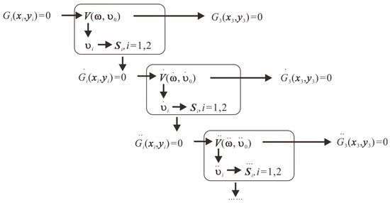
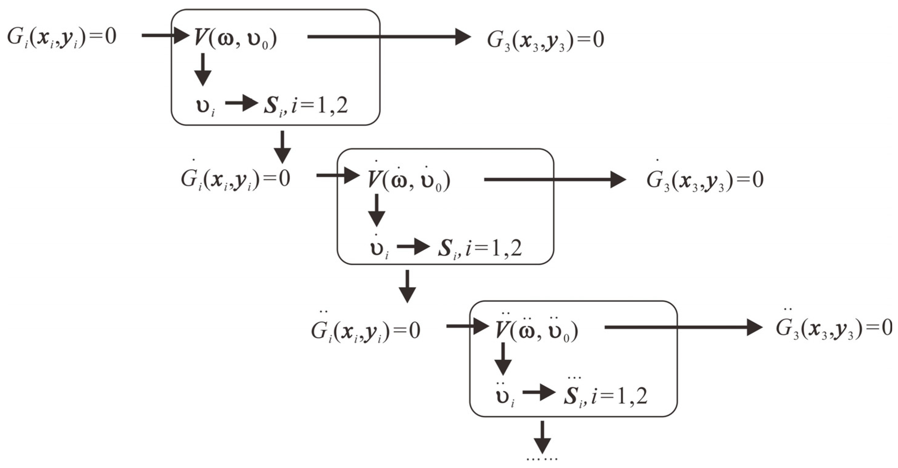
Equations (16)–(21) are a set of linear equations in terms of the velocity screws (and their higher-order terms). There is a gradual solution process for these equations. Suppose the configurations of the first two links are known, and the third link is unknown. The velocity screws of the platform can be determined by Equation (16) with an arbitrary constant. Application of this velocity screw to the derivative of geometric screws will lead to the second-order constraints. Higher-order constraints follow a similar way, as depicted by the flow chart in Figure 2.

Figure 2. Flow chart of the higher-order analysis.

2.2. Loci of Higher Order Curvature

Equations (16)–(21) are essential constraints on the locations of pivot points. Denote $\mathit{X}=\left\{{\mathit{x}}_j,{\mathit{y}}_j,j=1,2,3\right\}$ as the Cartesian coordinates and $\mathit{R}=\left\{r_j,{\theta }_j,j=1,2,3\right\}$ as the polar coordinates of the pivot points of the 3-RR linkages in the current configuration. For a planar platform shaky to the ith order, this requires that all the screws ${\mathit{S}}_i$ or the parameters $\mathit{X}$ of three chains satisfy constraints up to the ith order in Equations (16)–(21):

$$P_{\mathit{X}}^i=\left\{\mathit{X}|G_j=0,{\dot{G}}_j=0,\ddot{G_{\mathrm{j}}}=0,\cdots G_j^{(i-1)}=0,j=\mathrm{1,2},3\right\}.$$

(22)

The corresponding 3-RR linkages are further called shaky to the ith order, or ith-order infinitesimal mechanisms. The notation $P_{\mathit{R}}^i$ is used instead if polar coordinates are used.

Suppose the position of the third link is unknown. The locus of the couple points, ${\mathit{x}}_3$, and the corresponding center points, ${\mathit{y}}_3$, are subsets of the solution in Equation (22), i.e., the projections of the set $P_{\mathit{X}}^i$:

$$P_{{\mathit{x}}_3}^i={\mathrm{p}\mathrm{r}\mathrm{o}\mathrm{j}}_{{\mathit{x}}_3}\left(P_{\mathit{X}}^i\right),P_{{\mathit{y}}_3}^i={\mathrm{p}\mathrm{r}\mathrm{o}\mathrm{j}}_{{\mathit{y}}_3}\left(P_{\mathit{X}}^i\right).$$

(23)

The first-order solutions $P_{{\mathit{x}}_3}^1,P_{{\mathit{y}}_3}^1$ lead to the first-order contact i.e., having common tangents, between the path of the moving point ${\mathit{x}}_3$ and the circle centered at ${\mathit{y}}_3$ with radius equal to the length of the third link. Second-order solutions $P_{{\mathit{x}}_3}^2,P_{{\mathit{y}}_3}^2$ correspond to the second-order contact, that is to say, ${\mathit{y}}_3$ is center of curvature of the anchor point of ${\mathit{x}}_3$. Third-order solutions $P_{{\mathit{x}}_3}^3,P_{{\mathit{y}}_3}^3$ correspond to the third-order contact, and ${\mathit{x}}_3$ determines the locus of the cubic stationary curvature of the couple link, and ${\mathit{y}}_3$ is the curvature center. The merit of using Equation (22) is taking all the points of the four-bar linkage into consideration directly to determine the higher-order curvature of couple points and center points. In the following sections, the rotational and translational positions are investigated, respectively.

2.3. Transformation between Two Coordinate Systems

In classical curvature theory, the so-called canonical coordinate systems are usually used for the curvature analysis. It is also convenient to use other coordinate systems for some situations. Hence, the transformation between the two coordinate systems is analyzed firstly.

2.3.1. Rotational Position

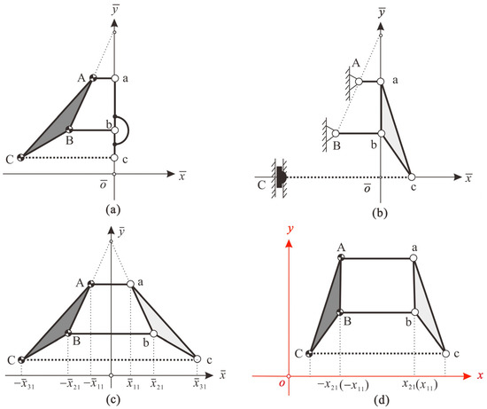
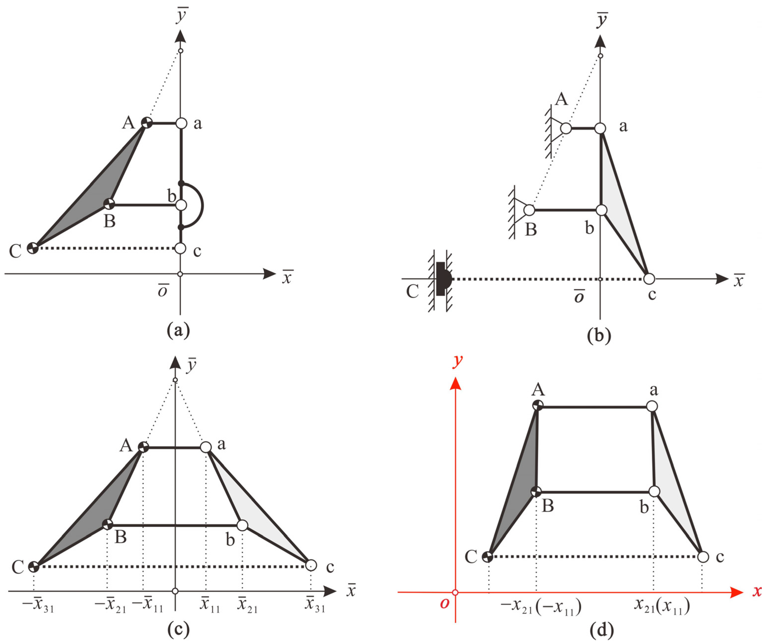
Suppose that the position of the four pivot points, i.e., b, B, A, and a, of a four-bar linkage are known, the position of the pivot points c and C are unknowns, and the pivots A, B, and C are denoted as the fixed points, as shown in Figure 3a. The canonical coordinates, denoted as $\sum \overline{x}\overline{o}\overline{y}$, are determined by the method of the so-called Bobillier’s construction [5]. The polar coordinates of the pivot points are denoted as $\left(r_{ij},{\overline{\theta }}_i\right)$ with respect to $\sum \overline{x}\overline{o}\overline{y}$. Therefore, the four-bar linkage has a total of six parameters, which exceeds the five required; thus, a constraint is placed on these parameters.

Figure 3. Coordinates of four-bar linkages, at (a) rotational and (b) translational position.

In order to apply canonical coordinates for the higher-order screw analysis with a minimum number of parameters, we use another coordinate system, called the natural coordinate system, denoted as $\sum xoy$. The origin of $\sum xoy$ is also located at the pole, and the x axis is collinear with the ray $\overrightarrow{PbB}$, as shown in Figure 3a. The polar coordinates of the pivots are denoted as $\mathrm{a}\left(r_{11},-{\theta }_1\right)$, $\mathrm{A}\left(r_{12},-{\theta }_1\right)$, $\mathrm{b}\left(r_{21},0\right)$, $\mathrm{B}\left(r_{22},0\right)$, $\mathrm{c}\left(r_{31},{\theta }_3\right)$, and $\mathrm{C}\left(r_{32},{\theta }_3\right)$, respectively, with respect to $\sum xoy$. Clearly, there are five parameters in total.

Referring to the coordinates $\sum xoy$, the intersection Q (collineation-point) of the ray $\overrightarrow{Pab}$ and $\overrightarrow{PAB}$ can be written as

$$\left\{\begin{array}{c}{x}_Q={\displaystyle \frac{r_{11}{r}_{12}{r}_{2}cos {\theta }_1-r_{21}{r}_{22}{r}_1}{r_{12}{r}_{21}-r_{11}{r}_{22}}},\\ y_Q=-{\displaystyle \frac{r_{11}{r}_{12}{r}_{2}sin {\theta }_1}{r_{12}{r}_{21}-r_{11}{r}_{22}}},\end{array}\right.$$

(24)

in which the notation $r_i$, defined as $r_i=r_{i1}-r_{i2}$, is used for brevity. The matrix that rotates the $\overline{x}$ axis of the canonical system $\sum \overline{x}\overline{o}\overline{y}$ to the ray $\overrightarrow{PaA}$ is a rotation of angle ${\overline{\theta }}_1$ about the pole

$$T_{0a}=\left(\begin{array}{cc}\mathrm{c}\mathrm{o}\mathrm{s}{\overline{\theta }}_1& -\mathrm{s}\mathrm{i}\mathrm{n}{\overline{\theta }}_1\\ \mathrm{s}\mathrm{i}\mathrm{n}{\overline{\theta }}_1& \mathrm{c}\mathrm{o}\mathrm{s}{\overline{\theta }}_1\end{array}\right)={\displaystyle \frac{1}{m}}\left(\begin{array}{cc}{\nu }_1& r_{11}{r}_{12}{r}_{2}sin{\theta }_1\\ -r_{11}{r}_{12}{r}_{2}sin{\theta }_1& {\nu }_1\end{array}\right),$$

(25)

in which the notation ${\nu }_1=r_{11}{r}_{12}{r}_{2}cos{\theta }_1-r_{21}{r}_{22}{r}_1$ and

$$m=\sqrt{r_{11}^2{r}_{12}^2{r}_2^2+r_{21}^2{r}_{22}^2{r}_1^2-2r_{11}{r}_{12}{r}_{21}{r}_{22}{r}_1{r}_{2}cos{\theta }_1}.$$

(26)

Then the transformation matrix $T_{0b}$ from $\sum \overline{x}\overline{o}\overline{y}$ to $\sum xoy$ can be obtained by multiplying a rotation of angle ${\theta }_1$ about the z axis, which is a rotation of angle ${\overline{\theta }}_2$ about the pole

$$T_{0b}=\left(\begin{array}{cc}\mathrm{c}\mathrm{o}\mathrm{s}{\overline{\theta }}_2& -\mathrm{s}\mathrm{i}\mathrm{n}{\overline{\theta }}_2\\ \mathrm{s}\mathrm{i}\mathrm{n}{\overline{\theta }}_2& \mathrm{c}\mathrm{o}\mathrm{s}{\overline{\theta }}_2\end{array}\right)={\displaystyle \frac{1}{m}}\left(\begin{array}{cc}{\nu }_2& r_{21}{r}_{22}{r}_{1}sin{\theta }_1\\ -r_{21}{r}_{22}{r}_{1}sin{\theta }_1& {\nu }_2\end{array}\right),$$

(27)

with the notation ${\nu }_2$ defined as ${\nu }_2=r_{11}{r}_{12}{r}_2-r_{21}{r}_{22}{r}_{1}cos{\theta }_1$. Then, the Cartesian coordinates $\left({\mathit{x}}_i,{\mathit{y}}_i\right)$ of the pivot points can be transformed from $\sum xoy$ to $\sum \overline{x}\overline{o}\overline{y}$ with a minimum number of parameters using Equation (27); the involved parameters $\left(r_{11},r_{12},r_{21},r_{22},{\theta }_1\right)$ are called the reduced canonical parameters in this paper. The quantities in Equations (16)–(21) can be expressed in $\sum xoy$ with the reduced canonical parameters, firstly, and then are transformed to $\sum \overline{x}\overline{o}\overline{y}$ by the matrix in Equation (27). Thus, the loci of higher order can be expressed in canonical coordinates but with reduced canonical parameters.

It should be noted that there will be at most one radial coordinate $r_{ij}$ equal to zero in order to form a feasible four-bar linkage. Furthermore, the angle ${\theta }_1$ between the two rays $\overrightarrow{PaA}$ and $\overrightarrow{PbB}$ is also assumed to be nonzero, excluding the case of folded four-bar linkages.

2.3.2. Translational Position

For the translational position of 3-RR linkages, the pole of the platform is at infinity, and thus has a translational mobility. The Cartesian coordinates of the pivots referring to a natural coordinate system $\sum xoy$ are denoted as a$\left(x_{11},y_1\right)$, A$\left(x_{12},y_1\right)$, b$\left(x_{21},y_2\right)$, B$\left(x_{22},y_2\right)$, c$\left(x_{31},y_3\right)$, and C$\left(x_{32},y_3\right)$, respectively. The abscissa axis $x$ is chosen to be parallel to one crank of the four-bar linkage, and the $y$ axis is perpendicular to it, as shown in Figure 3b.

In canonical systems $\sum \overline{x}\overline{o}\overline{y}$, the coordinates of the pivot points are denoted as $\left({\overline{x}}_{ij},{\overline{y}}_i\right)$, as shown by the black lines in Figure 3b. According to the Bobillier’s construction [6], the axis $\overline{y}$ passes the intersection of the ray $\overrightarrow{ab}$ and ray $\overrightarrow{AB}$, the axis $\overline{x}$ is aligned with the pole tangent and is the same distance away from the ray $\overrightarrow{bB}$ as the point Q (collineation-point) is from the ray $\overrightarrow{aA}$. The coordinates of the collineation point Q in $\sum xoy$ are

$$\left\{\begin{array}{c}{x}_Q={\displaystyle \frac{x_{11}{x}_{22}-x_{12}{x}_{21}}{x_{11}-x_{12}-x_{21}+x_{22}}},\\ y_Q={\displaystyle \frac{y_2\left(x_{11}-x_{12}\right)-y_1\left(x_{21}-x_{22}\right)}{x_{11}-x_{12}-x_{21}+x_{22}}}.\end{array}\right.$$

(28)

The equation of the pole tangent (also the degenerated inflection circle) is

$$y_P={\displaystyle \frac{y_1\left(x_{11}-x_{12}\right)-y_2\left(x_{21}-x_{22}\right)}{x_{11}-x_{12}-x_{21}+x_{22}}}.$$

(29)

If the previous relations are represented in the canonical system $\sum \overline{x}\overline{o}\overline{y}$, the coordinates of the pivot points in Equations (28) and (29) will be constrained by the relations ${\overline{x}}_Q=0$, ${\overline{y}}_P=0$, yielding

$$\left\{\begin{array}{c}{\overline{x}}_{11}={\overline{x}}_{21}{\overline{y}}_2/{\overline{y}}_1\\ {\overline{x}}_{12}={\overline{x}}_{22}{\overline{y}}_2/{\overline{y}}_1\end{array}\right., \mathrm{f}\mathrm{o}\mathrm{r} {\overline{x}}_{11}\ne {\overline{x}}_{21} \mathrm{o}\mathrm{r} {\overline{x}}_{12}\ne {\overline{x}}_{22}.$$

(30)

It is clear that ${\overline{y}}_1\ne {\overline{y}}_2\ne 0$ and ${\overline{x}}_{21}\ne {\overline{x}}_{22}$, which guarantees a feasible four-bar linkage at the translational position. Furthermore, if ${\overline{x}}_{11}={\overline{x}}_{21} \mathrm{o}\mathrm{r} {\overline{x}}_{12}={\overline{x}}_{22}$, the previous relations reduce to

$$\left\{\begin{array}{c}{\overline{x}}_{11}={\overline{x}}_{21}=0,\\ {\overline{x}}_{12}={\overline{y}}_2{\overline{x}}_{22}/{\overline{y}}_1,\end{array}\right. \mathrm{o}\mathrm{r} \left\{\begin{array}{c}{\overline{x}}_{11}={\overline{y}}_2{\overline{x}}_{21}/{\overline{y}}_1,\\ {\overline{x}}_{12}={\overline{x}}_{22}=0.\end{array}\right.$$

(31)

These constraints imply that only four parameters, $\left({\overline{x}}_{21},{\overline{x}}_{22},{\overline{y}}_2,{\overline{y}}_1\right)$, are necessary to determine the configuration of the four-bar linkage in translational position. The parameters $\left({\overline{x}}_{21},{\overline{x}}_{22},{\overline{y}}_2,{\overline{y}}_1\right)$ are called the reduced canonical parameters at the translational position. Furthermore, application of the coordinates in Equation (30) to the $y$ component of the collineation point Q yields ${\overline{y}}_Q={\overline{y}}_1+{\overline{y}}_2$.

3. Results

Building upon the frameworks of the previous sections, the loci of higher-order curvature of four-bar linkages can be obtained to arbitrary order using the reduced canonical parameters. In the following, some analytical solutions are presented for the rotational position up to the third order and the translational position up to the sixth order. Some results have not been reported in the literature.

3.1. Formulae for Rotational Position

3.1.1. New Euler–Savary Equation

The first-order analysis is trivial, since the third link axis also intersects at the pole. The second-order analysis is related to the curvature of the couple point, i.e., the Euler–Savary equation. Representing the Cartesian coordinates of points $a,b,A,B,$ c, and C in $\sum xoy$, the second-order constraint $P_{\left\{r_{31},r_{32},{\mathsf{\theta }}_3\right\}}^2$ yields a new version of the Euler–Savary equation:

$${\displaystyle \frac{sin {\theta }_1}{\frac{1}{r_{31}}-\frac{1}{r_{32}}}}+{\displaystyle \frac{sin {\theta }_3}{\frac{1}{r_{11}}-\frac{1}{r_{12}}}}-{\displaystyle \frac{sin \left({\theta }_1+{\theta }_3\right)}{\frac{1}{r_{21}}-\frac{1}{r_{22}}}}=0,$$

(32)

which relates the couple point $c\left(r_{31},{\theta }_3\right)$ to its center of curvature $C\left(r_{32},{\mathsf{\theta }}_3\right)$ to the second order.

Using the transformation, ${\overline{\theta }}_3-{\overline{\theta }}_2={\theta }_3$, Equation (32) can be rewritten as

$${\displaystyle \frac{1}{r_{31}}}-{\displaystyle \frac{1}{r_{32}}}={\displaystyle \frac{1}{Dsin {\overline{\theta }}_3}},$$

(33)

which is the classic form of the Euler–Savary equation. The term $D$ (also the instantaneous invariant $b_2$) in Equation (33) is the diameter of the inflection circle (i.c. for short), which can be expressed with reduced canonical parameters as

$$D=b_2={\displaystyle \frac{1}{sin {\theta }_1}}\sqrt{{\displaystyle \frac{1}{{\left(\frac{1}{r_{21}}-\frac{1}{r_{22}}\right)}^2}}+{\displaystyle \frac{1}{{\left(\frac{1}{r_{11}}-\frac{1}{r_{12}}\right)}^2}}-{\displaystyle \frac{2cos {\theta }_1}{\left(\frac{1}{r_{21}}-\frac{1}{r_{22}}\right)\left(\frac{1}{r_{11}}-\frac{1}{r_{12}}\right)}}}={\displaystyle \frac{m}{r_1{r}_{2}sin {\theta }_1}}.$$

(34)

The i.c. curve, represented with variables $\left(r_{31},{\overline{\theta }}_3\right)$, can be obtained by the vanishing of $1/r_{32}$ in Equation (33):

$$r_{31}=Dsin {\overline{\theta }}_3.$$

(35)

Apply Equation (33) to the three pair of pivot points,

$${\displaystyle \frac{1}{\frac{1}{r_{11}}-\frac{1}{r_{12}}}}=Dsin {\overline{\theta }}_1,{\displaystyle \frac{1}{\frac{1}{r_{21}}-\frac{1}{r_{22}}}}=Dsin {\overline{\theta }}_2,{\displaystyle \frac{1}{\frac{1}{r_{31}}-\frac{1}{r_{32}}}}=Dsin {\overline{\theta }}_3.$$

(36)

Then, multiply both sides of the three equations by $sin \left({\overline{\theta }}_3-{\overline{\theta }}_2\right)$, $sin \left({\overline{\theta }}_1-{\overline{\theta }}_3\right)$, and $sin\left({\overline{\theta }}_2-{\overline{\theta }}_1\right)$, respectively, and make summations; the right-hand side will vanish, and

$$\begin{array}{c}{\displaystyle \frac{sin \left({\overline{\theta }}_3-{\overline{\theta }}_2\right)}{\frac{1}{r_{11}}-\frac{1}{r_{12}}}}+{\displaystyle \frac{sin \left({\overline{\theta }}_1-{\overline{\theta }}_3\right)}{\frac{1}{r_{21}}-\frac{1}{r_{22}}}}+{\displaystyle \frac{sin \left({\overline{\theta }}_2-{\overline{\theta }}_1\right)}{\frac{1}{r_{31}}-\frac{1}{r_{32}}}}=\\ Dsin {\overline{\theta }}_{1}sin \left({\overline{\theta }}_3-{\overline{\theta }}_2\right)+Dsin {\overline{\theta }}_{2}sin \left({\overline{\theta }}_1-{\overline{\theta }}_3\right)+Dsin {\overline{\theta }}_{3}sin \left({\overline{\theta }}_2-{\overline{\theta }}_1\right)=0.\end{array}$$

(37)

The arguments of the sines in Equation (37) satisfy ${\overline{\theta }}_2-{\overline{\theta }}_1={\theta }_1$, ${\overline{\theta }}_3-{\overline{\theta }}_2={\theta }_3$, and ${\overline{\theta }}_1-{\overline{\theta }}_3=-\left({\theta }_1+{\theta }_3\right)$, representing the angles between two adjacent rays. Consequently, the new Euler–Savary equation in Equation (32) is recovered again, without referring to the canonical coordinates.

Clearly, no instantaneous invariants or canonical coordinates are used in Equations (32) or (37), thus, offering an efficient formula to determine the center of curvature of a four-bar linkage. To the best knowledge of the authors, Equations (32) or (37) have not yet been reported in literature despite their simplicity and conciseness. Furthermore, Equation (32) is also the constraint imposed on the three pairs of pivot points that must be fulfilled in order for the corresponding 3-RR linkages to be shaky to the second order.

3.1.2. Cubic of Stationary Curvature

The intersection of the second- and third-order constraints, i.e., $P_{\left\{r_{31},r_{32},{\overline{\theta }}_3\right\}}^3$, gives rise to the cubic of stationary curvature and corresponding center of curvature. The former curve is also called the circling point curve ($\mathrm{c}\mathrm{p}$ for short); the latter one is the center point curve ($\widetilde{\mathrm{c}\mathrm{p}}$ for short). Referring to the canonical coordinates $\sum \overline{x}\overline{o}\overline{y}$, the two curves can be written compactly with reduced canonical parameters as

$$\left\{\begin{array}{c}\mathrm{c}\mathrm{p}\left(r_{31},{\overline{\theta }}_3\right):{\displaystyle \frac{m^3}{r_{31}}}={\displaystyle \frac{{\mu }_0{\mu }_1{\mu }_2}{sin {\overline{\theta }}_3}}+{\displaystyle \frac{{\nu }_0{\nu }_1{\nu }_2}{cos {\overline{\theta }}_3}},\\ \widetilde{\mathrm{c}\mathrm{p}}\left(r_{32},{\overline{\theta }}_3\right):{\displaystyle \frac{m^3}{r_{32}}}={\displaystyle \frac{{\mu }_0^{\mathrm{\prime }}{\mu }_1^{\mathrm{\prime }}{\mu }_2^{\mathrm{\prime }}}{sin {\overline{\theta }}_3}}+{\displaystyle \frac{{\nu }_0{\nu }_1{\nu }_2}{cos {\overline{\theta }}_3}},\end{array}\right.$$

(38)

in which the coefficient $m$ is given in Equation (26); other coefficients can be written as

$$\left\{\begin{array}{c}{\nu }_0=r_{12}{r}_{21}-r_{11}{r}_{22},\\ {\nu }_1=r_{11}{r}_{12}{r}_{2}cos {\theta }_1-r_{21}{r}_{22}{r}_1,\\ {\nu }_2=r_{11}{r}_{12}{r}_2-r_{21}{r}_{22}{r}_{1}cos {\theta }_1,\end{array}\right.$$

(39)

$$\left\{\begin{array}{c}{\mu }_0=\left[\left(r_{22}{r}_1+r_{12}{r}_2\right)r_{11}{r}_{21}cos {\theta }_1-r_{11}^2{r}_{12}{r}_2-r_{21}^2{r}_{22}{r}_1\right]r_1{r}_{2}sin {\theta }_1,\\ {\mu }_1=r_{12},\\ {\mu }_2=r_{22},\end{array}\right.$$

(40)

$$\left\{\begin{array}{c}{\mu }_0^{\mathrm{\prime }}=\left[\left({r_{21}{r}_1+r}_{11}{r}_2\right)r_{12}{r}_{22}cos {\theta }_1-r_{11}{r}_{12}^2{r}_2-r_{21}{r}_{22}^2{r}_1\right]r_1{r}_{2}sin {\theta }_1,\\ {\mu }_1^{\mathrm{\prime }}=r_{11},\\ {\mu }_2^{\mathrm{\prime }}=r_{21}.\end{array}\right.$$

(41)

It is noted that none of the terms ${\mu }_0^{\mathrm{\prime }},{\mu }_0,{\nu }_0,{\nu }_1 \mathrm{o}\mathrm{r} {\nu }_2$ will vanish if any single radius vanishes: $r_{ij}=0$. Denote $\mu ={\mu }_0{\mu }_1{\mu }_2$, ${\mu }^{\mathrm{\prime }}={\mu }_0^{\mathrm{\prime }}{\mu }_1^{\mathrm{\prime }}{\mu }_2^{\mathrm{\prime }}$, and $\nu ={\nu }_0{\nu }_1{\nu }_2$; it can be seen that

$$\mu -{\mu }^{\mathrm{\prime }}=m^3/D,$$

(42)

which is a well-known identity.

Make notations $k_{ij}=1/r_{ij}$, $k_i=1/r_{i1}-1/r_{i2}$, and

$$\left\{\begin{array}{c}{V}_0=k_{11}{k}_{22}-k_{12}{k}_{21},\\ V_1=k_1-k_{2}cos {\theta }_1,\\ V_2=k_{1}cos {\theta }_1-k_2,\end{array}\right.\left\{\begin{array}{c}U=k_{1}sin {\theta }_1\left[k_{21}\left(V_2^2+{k_1^{2}sin}^2 {\theta }_1\right)-V_0{V}_1\right],\\ \begin{array}{c}{U}^{\mathrm{\prime }}=k_{1}sin {\theta }_1\left[k_{22}\left(V_2^2+{k_1^{2}sin}^2 {\theta }_1\right)-V_0{V}_1\right]\\ M={\left(V_2^2+{k_1^{2}sin}^2 {\theta }_1\right)}^{0.5}.\end{array}\end{array},\right.$$

(43)

If we also represent the unknown pivot points c and C in $\sum xoy$, the two cubics $\mathrm{c}\mathrm{p}\left(r_{31},{\theta }_3\right)$ and $\widetilde{\mathrm{c}\mathrm{p}}\left(r_{32},{\theta }_3\right)$ will become

$$\left\{\begin{array}{c}{\displaystyle \frac{1}{r_{31}}}={\displaystyle \frac{V_0{V}_{1}sin {\theta }_3+k_{21}{k}_{1}sin {\theta }_1\left(V_{2}cos {\theta }_3-k_{1}sin {\theta }_{1}sin {\theta }_3\right)}{\left(V_{2}sin {\theta }_3+k_{1}sin {\theta }_{1}cos {\theta }_3\right)\left(V_{2}cos {\theta }_3-k_{1}sin {\theta }_{1}sin {\theta }_3\right)}}={\displaystyle \frac{1}{M^3}}\left[{\displaystyle \frac{U}{sin \left({\theta }_3+\mathrm{\varnothing }\right)}}+{\displaystyle \frac{V_0{V}_1{V}_2}{cos \left({\theta }_3+\mathrm{\varnothing }\right)}}\right],\\ {\displaystyle \frac{1}{r_{32}}}={\displaystyle \frac{V_0{V}_{1}sin {\theta }_3+k_{22}{k}_{1}sin {\theta }_1\left(V_{2}cos {\theta }_3-k_{1}sin {\theta }_{1}sin {\theta }_3\right)}{\left(V_{2}sin {\theta }_3+k_{1}sin {\theta }_{1}cos {\theta }_3\right)\left(V_{2}cos {\theta }_3-k_{1}sin {\theta }_{1}sin {\theta }_3\right)}}={\displaystyle \frac{1}{M^3}}\left[{\displaystyle \frac{U^{\mathrm{\prime }}}{sin \left({\theta }_3+\mathrm{\varnothing }\right)}}+{\displaystyle \frac{V_0{V}_1{V}_2}{cos \left({\theta }_3+\mathrm{\varnothing }\right)}}\right],\end{array}\right.$$

(44)

respectively, in which ${\theta }_3+\mathrm{\varnothing }={\overline{\theta }}_3$ and $cos\mathrm{\varnothing }=V_2/M,sin \mathrm{\varnothing }=k_{1}sin {\theta }_1/M$ are equal to the two entries in the first column of the matrix (27), respectively. Hence, the two Equations (38) and (44) are essentially equivalent, with the correspondences $V_i\leftrightarrow {\nu }_i$, $U\leftrightarrow \mu$, and $U^{\mathrm{\prime }}\leftrightarrow {\mu }^{\mathrm{\prime }}$ under the transformation ${\theta }_3+\mathrm{\varnothing }\to {\overline{\theta }}_3$.

The intersection of the inflection circle in Equation (35) (or Equation (32)) and cubics of stationary curvatures in Equation (38) (or Equation (44)) gives rise to the Ball’s point, which has instantaneous infinite curvature. In this condition, the corresponding fixed pivot of 3-RR linkages approaches infinity. With respect to the canonical systems, the angular location of Ball’s point can be written as

$$tan {\overline{\theta }}_3={\displaystyle \frac{m^2-D{\mu }_0{\mu }_1{\mu }_2}{D{\nu }_0{\nu }_1{\nu }_2}}.$$

(45)

The radial coordinates of the Ball’s point are determined by Equations (38) or (44). With respect to the natural coordinates, the angular location ${\theta }_3$ of the Ball’s point can be obtained with Equation (45) and the relation $\mathrm{t}\mathrm{a}\mathrm{n} \left({\overline{\theta }}_3-{\overline{\theta }}_2\right)=\mathrm{t}\mathrm{a}\mathrm{n} {\theta }_3$, and the term $\mathrm{t}\mathrm{a}\mathrm{n} {\overline{\theta }}_2$ can be calculated by the entries of the matrix in Equation (27).

3.1.3. Classification of the Degenerate Cubics

It is known that the cubic of stationary curves of four-bar linkages will degenerate into a circle and a line (its extended diameters) if the coefficients in the denominators of Equations (38) or (44) vanish. Thanks to the explicit expressions of factors of $\mu$, ${\mu }^{\mathrm{\prime }}$, and $\nu$ in Equation (38), a complete classification of the degenerate cubics can be obtained.

There are generally two classes of degenerations, both for $\mathrm{c}\mathrm{p}$ and $\widetilde{\mathrm{c}\mathrm{p}}$; the first case is $\mu \mathrm{o}\mathrm{r} {\mu }^{\mathrm{\prime }}=0$, in which the degenerate line is collinear with the pole tangent; the second case is $\nu =0$ (also called the cycloidal position), in which $\mathrm{c}\mathrm{p}$ and $\widetilde{\mathrm{c}\mathrm{p}}$ will both degenerate with the degenerate lines aligning with the pole norm. Furthermore, the i.c. will have a common tangent, i.e., the pole tangent at the pole with $\mathrm{c}\mathrm{p}$ and $\widetilde{\mathrm{c}\mathrm{p}}$ if $\nu =0$; hence, the only Ball’s point will be the inflection pole (the intersection of the pole norm and i.c.), other than the velocity pole. The previous two classes can be further divided into three subclasses corresponding to the vanishing of factors ${\mu }_k=0$ or ${\nu }_k=0$, $k=0,1,2$ for $\mathrm{c}\mathrm{p}$ and ${\mu }_k^{\mathrm{\prime }}=0$ or ${\nu }_k=0,$ $k=0,1,2$ for $\widetilde{\mathrm{c}\mathrm{p}}$. Choosing a suitable independent variable in the constraints formed by the vanishing of these factors in Equations (39)–(41), the expressions of the six degenerate cubics of $\mathrm{c}\mathrm{p}$ and $\widetilde{\mathrm{c}\mathrm{p}}$ are given in the following.

• ${\mu }_0=0$ or ${\mu }_0^{\mathrm{\prime }}=0$

The $\mathrm{c}\mathrm{p}$ curve will degenerate if ${\mu }_0=0$; however, the center point curve $\widetilde{\mathrm{c}\mathrm{p}}\left(r_{31},{\theta }_3\right)$ will not degenerate, and the collineation line $\overrightarrow{PQ}$ will be perpendicular to the moving link $ab$. The $\widetilde{\mathrm{c}\mathrm{p}}$ curve will degenerate if ${\mu }_0^{\mathrm{\prime }}=0$ while the $\mathrm{c}\mathrm{p}$ curve remains a cubic, and the collineation line $\overrightarrow{PQ}$ will then be perpendicular to the fixed link $AB$. The equations of degenerate cubics and the corresponding inflection circle in terms of $\left(r_{31},{\overline{\theta }}_3\right)$ are

$$\mathrm{i}\mathrm{f} {\mu }_0=0⟹\left\{\begin{array}{c}\mathrm{c}\mathrm{p}:r_{31}={\displaystyle \frac{cos {\overline{\theta }}_3\sqrt{r_{11}^2+r_{21}^2-2r_{11}{r}_{21}cos {\theta }_1}}{sin {\theta }_1}}={\displaystyle \frac{\left|\overrightarrow{ab}\right|cos {\overline{\theta }}_3}{sin {\theta }_1}}, \mathrm{o}\mathrm{r} {\overline{\theta }}_3=0,\\ \mathrm{i}.\mathrm{c}.:r_{31}={\displaystyle \frac{r_{21}{r}_{22}\left|\overrightarrow{ab}\right|sin {\overline{\theta }}_3}{\left(r_{11}-r_{21}cos {\theta }_1\right)\left(r_{22}-r_{21}\right)}},\end{array}\right.$$

(46)

$$\mathrm{i}\mathrm{f} {\mu }_0^{\mathrm{\prime }}=0⟹\left\{\begin{array}{c}\widetilde{\mathrm{c}\mathrm{p}}:r_{32}={\displaystyle \frac{cos {\overline{\theta }}_3\sqrt{r_{12}^2+r_{22}^2-2r_{12}{r}_{22}cos {\theta }_1}}{sin {\theta }_1}}={\displaystyle \frac{\left|\overrightarrow{AB}\right|cos {\overline{\theta }}_3}{sin {\theta }_1}}, \mathrm{o}\mathrm{r} {\overline{\theta }}_3=0,\\ \mathrm{i}.\mathrm{c}.:r_{31}={\displaystyle \frac{r_{21}{r}_{22}\left|\overrightarrow{AB}\right|sin {\overline{\theta }}_3}{\left(r_{12}-r_{22}cos {\theta }_1\right)\left(r_{22}-r_{21}\right)}}.\end{array}\right.$$

(47)

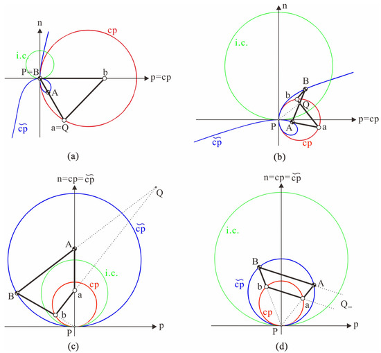
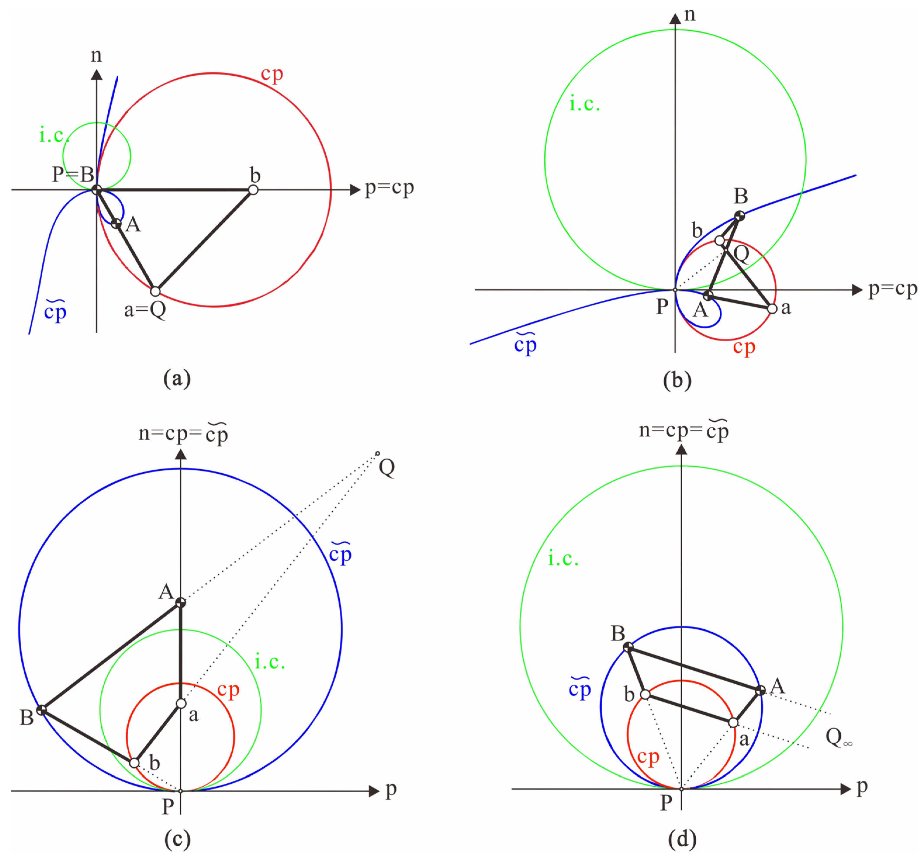
An example for ${\mu }_0=0$ is shown in Figure 4b, and the parameters are specified as $r_{11}=6$, $r_{12}=2$, $r_{21}=4$, $r_{22}=6$, and ${\theta }_1=\pi /3$ (the units are omitted without loss of generality).

Figure 4. Degenerate cubics for the rotational position, (a) $r_{22}=0$, (b) ${\mu }_0=0$, (c) ${\nu }_1=0$, (d) ${\nu }_0=0$.

ii.

$r_{i1}=0$ or $r_{i2}=0$

On the condition of $r_{ij}=0$, the velocity pole of the four-bar linkage will be coincident with the pivot point which has the vanishing radius $r_{ij}=0$. For condition $r_{i1}=0$ (or $r_{i2}=0$), the center point curve $\widetilde{cp}$ (or $cp$ curve) will degenerate into a circle and a line identical to the pole tangent. It can be shown that the pole tangent will align with the ray $\overrightarrow{\mathrm{P}\mathrm{b}\mathrm{B}}$, if $r_{2i}=0$, and will align with $\overrightarrow{\mathrm{P}\mathrm{a}\mathrm{A}}$ if $r_{1i}=0$ on inspection of the transformation matrix in Equations (25) and (27). The degenerate cubics and the corresponding inflection circle are

$$\mathrm{i}\mathrm{f} r_{i2}=0, \left(i\ne j,\in \left\{\mathrm{1,2}\right\}\right)⟹\left\{\begin{array}{c}\mathrm{c}\mathrm{p}:r_{31}={\left(-1\right)}^i{\displaystyle \frac{r_{j1}cos {\overline{\theta }}_3}{cos{\theta }_1}}, \mathrm{o}\mathrm{r} {\overline{\theta }}_3=0\left(\mathrm{t}\mathrm{h}\mathrm{e} i\mathrm{t}\mathrm{h} \mathrm{r}\mathrm{a}\mathrm{y}\right),\\ \mathrm{i}.\mathrm{c}.:r_{31}={\displaystyle \frac{r_{j1}{r}_{j2}sin {\overline{\theta }}_3}{sin {\theta }_1\left(r_{j1}-r_{j2}\right)}},\end{array}\right.$$

(48)

$$\mathrm{i}\mathrm{f} r_{i1}=0, \left(i\ne j,\in \left\{\mathrm{1,2}\right\}\right)⟹\left\{\begin{array}{c}\widetilde{\mathrm{c}\mathrm{p}}:r_{32}={\left(-1\right)}^j{\displaystyle \frac{r_{j2}cos {\overline{\theta }}_3}{cos {\theta }_1}}, \mathrm{o}\mathrm{r} {\overline{\theta }}_3=0\left(\mathrm{t}\mathrm{h}\mathrm{e} i\mathrm{t}\mathrm{h} \mathrm{r}\mathrm{a}\mathrm{y}\right),\\ \mathrm{i}.\mathrm{c}.:r_{31}={\displaystyle \frac{r_{j1}{r}_{j2}sin {\overline{\theta }}_3}{sin {\theta }_1\left(r_{j2}-r_{j1}\right)}}.\end{array}\right.$$

(49)

An example for $r_{22}=0$ is shown in Figure 4a, and rest of the parameters are specified as $r_{21}=4$, $r_{11}=3$, $r_{12}=1$, and ${\theta }_1=\pi /3$.

iii.

${\nu }_0=0$

In this condition, the two lines $\overrightarrow{ab}$ and $\overrightarrow{AB}$ are parallel with each other, and the $\mathrm{c}\mathrm{p}$ and $\widetilde{\mathrm{c}\mathrm{p}}$ curves will both degenerate into a circle and a line:

$$\left\{\begin{array}{c}\mathrm{c}\mathrm{p}:r_{31}={\displaystyle \frac{sin {\overline{\theta }}_3\sqrt{r_{11}^2+r_{21}^2-2r_{11}{r}_{21}cos{\theta }_1}}{sin {\theta }_1}}={\displaystyle \frac{\left|\overrightarrow{ab}\right|sin {\overline{\theta }}_3}{sin{\theta }_1}}, \mathrm{o}\mathrm{r} {\overline{\theta }}_3={\displaystyle \frac{\pi }{2}},\\ \begin{array}{c}\widetilde{\mathrm{c}\mathrm{p}}:r_{32}={\displaystyle \frac{sin {\overline{\theta }}_3\sqrt{r_{12}^2+r_{22}^2-2r_{12}{r}_{22}cos{\theta }_1}}{sin {\theta }_1}}={\displaystyle \frac{\left|\overrightarrow{AB}\right|sin {\overline{\theta }}_3}{sin {\theta }_1}}, \mathrm{o}\mathrm{r} {\overline{\theta }}_3={\displaystyle \frac{\pi }{2}},\\ \mathrm{i}.\mathrm{c}.:r_{31}={\displaystyle \frac{r_{21}\left|\overrightarrow{AB}\right|sin {\overline{\theta }}_3}{sin {\theta }_1\left(r_{22}-r_{21}\right)}}.\end{array}\end{array}\right.$$

(50)

An example is shown in Figure 4d, with parameters $r_{11}=10/3$, $r_{12}=5$, $r_{21}=4$, $r_{22}=6$, and ${\theta }_1=\pi /3$.

iv.

${\nu }_1=0$

At this condition, the $\mathrm{c}\mathrm{p}$ and $\widetilde{\mathrm{c}\mathrm{p}}$ curves will both degenerate into a circle and a line aligned with the pole norm, which also coincides with the ray $\overrightarrow{\mathrm{P}\mathrm{a}\mathrm{A}}$, and the collineation line $\overrightarrow{PQ}$ will be perpendicular to the ray $\overrightarrow{\mathrm{P}\mathrm{b}\mathrm{B}}$:

$$\left\{\begin{array}{c}\mathrm{c}\mathrm{p}:r_{31}={\displaystyle \frac{r_{21}sin {\overline{\theta }}_3}{cos {\theta }_1}}, \mathrm{o}\mathrm{r} {\overline{\theta }}_3={\displaystyle \frac{\pi }{2}}\left(\mathrm{t}\mathrm{h}\mathrm{e} \mathrm{r}\mathrm{a}\mathrm{y} \overrightarrow{\mathrm{P}\mathrm{a}\mathrm{A}}\right),\\ \begin{array}{c}\begin{array}{c}\widetilde{\mathrm{c}\mathrm{p}}:r_{32}={\displaystyle \frac{r_{22}sin {\overline{\theta }}_3}{cos {\theta }_1}}, \mathrm{o}\mathrm{r} {\overline{\theta }}_3={\displaystyle \frac{\pi }{2}}\left(\mathrm{t}\mathrm{h}\mathrm{e} \mathrm{r}\mathrm{a}\mathrm{y} \overrightarrow{\mathrm{P}\mathrm{a}\mathrm{A}}\right),\\ \mathrm{i}.\mathrm{c}.:r_{31}={\displaystyle \frac{r_{21}{r}_{22}sin {\overline{\theta }}_3}{\left(r_{22}-r_{21}\right)cos {\theta }_1}}.\end{array}\\ \end{array}\end{array}\right.$$

(51)

An example is shown in Figure 4c, with parameters $r_{11}=42/13$, $r_{12}=7$, $r_{21}=2$, $r_{22}=6$, and ${\theta }_1=\pi /3$.

v.

${\nu }_2=0$

Similar to the case ${\nu }_1=0$, the $\mathrm{c}\mathrm{p}$ and $\widetilde{\mathrm{c}\mathrm{p}}$ curves will both degenerate into a circle and a line aligned with the pole norm, which also coincides with the ray $\overrightarrow{\mathrm{P}\mathrm{b}\mathrm{B}}$, and the collineation line $\overrightarrow{PQ}$ will be perpendicular to the ray $\overrightarrow{\mathrm{P}\mathrm{a}\mathrm{A}}$:

$$\left\{\begin{array}{c}\mathrm{c}\mathrm{p}:r_{31}={\displaystyle \frac{r_{11}sin {\overline{\theta }}_3}{cos{\theta }_1}}, \mathrm{o}\mathrm{r} {\theta }_3={\displaystyle \frac{\pi }{2}}\left(\mathrm{t}\mathrm{h}\mathrm{e} \mathrm{r}\mathrm{a}\mathrm{y} \overrightarrow{\mathrm{P}\mathrm{b}\mathrm{B}}\right),\\ \begin{array}{c}\widetilde{\mathrm{c}\mathrm{p}}:r_{32}={\displaystyle \frac{r_{12}sin {\overline{\theta }}_3}{cos{\theta }_1}}, \mathrm{o}\mathrm{r} {\theta }_3={\displaystyle \frac{\pi }{2}}\left(\mathrm{t}\mathrm{h}\mathrm{e} \mathrm{r}\mathrm{a}\mathrm{y} \overrightarrow{\mathrm{P}\mathrm{b}\mathrm{B}}\right),\\ \mathrm{i}.\mathrm{c}.:r_{31}={\displaystyle \frac{r_{11}{r}_{12}sin {\overline{\theta }}_3}{\left(r_{12}-r_{11}\right)cos {\theta }_1}}.\end{array}\end{array}\right.$$

(52)

vi.

$\mu \mathrm{o}\mathrm{r} {\mu }^{\mathrm{\prime }}=0$ and $\nu =0$

Since the four relations ${\mu }_0^{\mathrm{\prime }}=0, {\mu }_0=0, {\nu }_1=0, \mathrm{a}\mathrm{n}\mathrm{d} {\nu }_2=0$ represent the perpendicularity of the collineation line to the four sides of the four-bar linkage, respectively, no two of these relations can hold simultaneously. Hence, the only feasible combination of $\mu \mathrm{o}\mathrm{r} {\mu }^{\mathrm{\prime }}=0$ and $\nu =0$ is $\left\{{\mu }_1^{\mathrm{\prime }},{\mu }_2^{\mathrm{\prime }},{\mu }_1 \mathrm{o}\mathrm{r} {\mu }_2=0\right\}$ or $\left\{{\nu }_1 \mathrm{o}\mathrm{r} {\nu }_2=0\right\}$. This can be achieved by $r_{ij}=0$ and ${\theta }_1=\pi /2$ (other conditions may exist), considering Equation (39). For the combination ${\mu }^{\mathrm{\prime }}=0, \nu =0$ (also called Cardan position), the curve $\widetilde{\mathrm{c}\mathrm{p}}$ degenerates into the lines of the pole tangent, the pole norm, and the ideal line at infinity, and the $\mathrm{c}\mathrm{p}$ will become

$$\mathrm{c}\mathrm{p}:r_{31}={\displaystyle \frac{r_{i1}{r}_{i2}sin{\overline{\theta }}_3}{r_{i2}-r_{i1}}}, \mathrm{o}\mathrm{r} {\overline{\theta }}_3={\displaystyle \frac{\pi }{2}}, \mathrm{i}\mathrm{f} r_{j1}=0, {\theta }_1={\displaystyle \frac{\pi }{2}}, \left(i\ne j,\in \left\{\mathrm{1,2}\right\}\right),$$

(53)

in which the circle-component of $\mathrm{c}\mathrm{p}$ is identical to the inflection circle, according to the relation in Equation (42). For combination $\mu =0, \nu =0$ (also called the cardioidal position), the curve $\mathrm{c}\mathrm{p}$ will degenerate into three lines and the $\widetilde{\mathrm{c}\mathrm{p}}$ has a similar expression as that in Equation (53):

$$\widetilde{\mathrm{c}\mathrm{p}}:r_{32}={\displaystyle \frac{r_{i1}{r}_{i2}sin{\overline{\theta }}_3}{r_{i2}-r_{i1}}}, \mathrm{o}\mathrm{r} {\overline{\theta }}_3={\displaystyle \frac{\pi }{2}}, \mathrm{i}\mathrm{f} r_{j2}=0, {\theta }_1={\displaystyle \frac{\pi }{2}}, \left(i\ne j,\in \left\{\mathrm{1,2}\right\}\right),$$

(54)

whose circle component is identical to the inflection circle but with opposite sign. The pole tangents of the previous two cases are similar to those in cases ii; say the pole tangent will align with the ray $\overrightarrow{\mathrm{P}\mathrm{b}\mathrm{B}}$, if $r_{2i}=0$, and align with $\overrightarrow{\mathrm{P}\mathrm{a}\mathrm{A}}$ if $r_{1i}=0$.

The previous degenerate cubics have already been discussed case-by-case in [2,6] with instantaneous invariants, not the geometric parameters of the four-bar linkages. This paper presents a complete and neat algebraic classification in terms of concrete geometric parameters in Equations (38) and (44), which is of pedagogical value.

3.1.4. An Example of Straight-Line Mechanisms

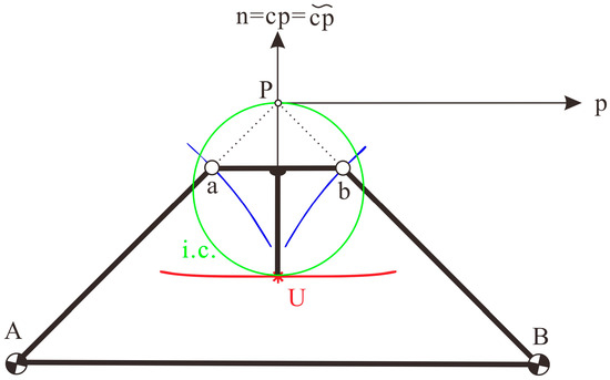
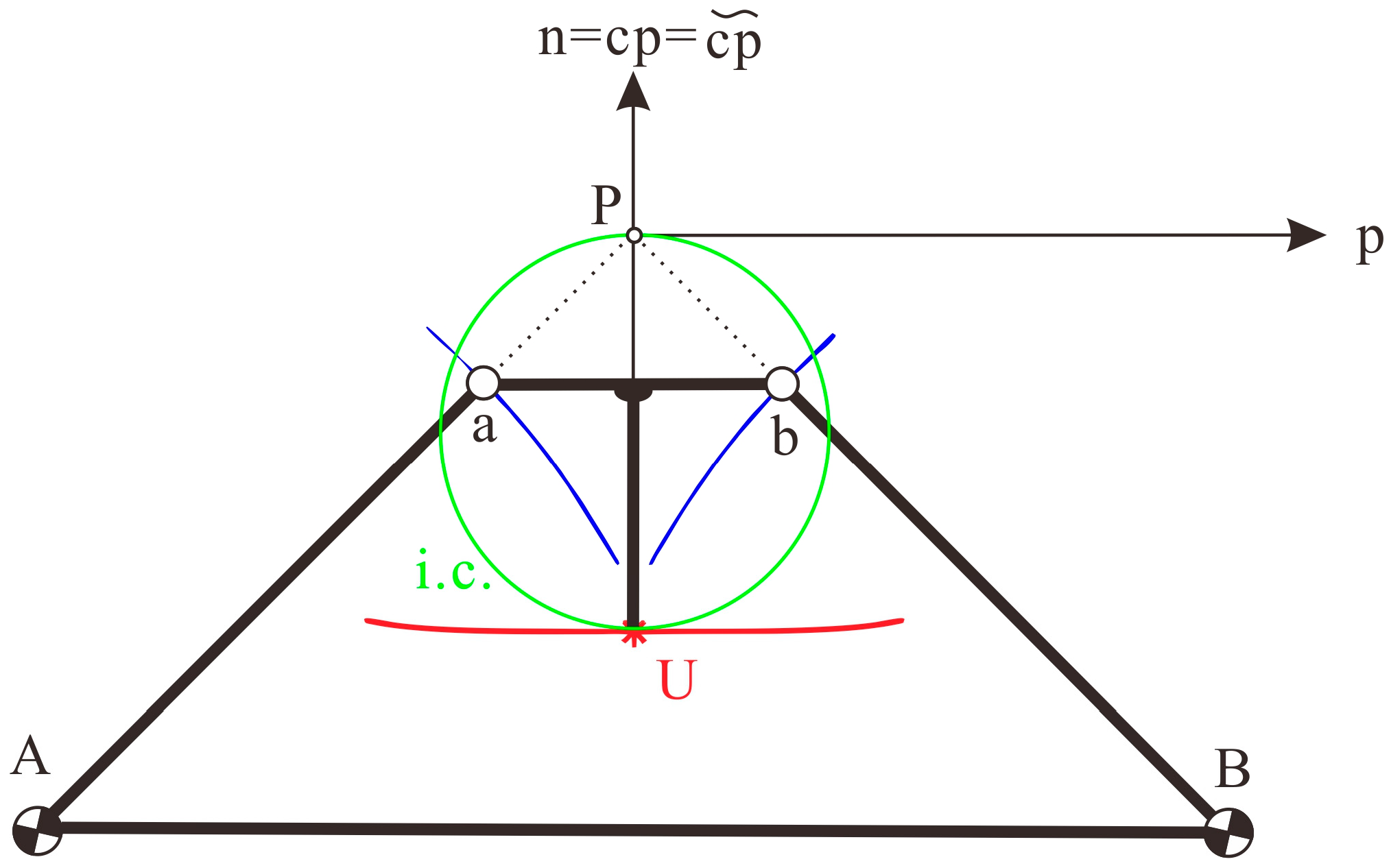
It is known that the Ball’s points can trace at least four-point contact with its tangent line, and is used for generating approximate straight lines. An example is shown in the following. The two rays of the exemplified four-bar linkage are perpendicular with each other i.e., $\overrightarrow{\mathrm{P}\mathrm{b}\mathrm{B}}\perp \overrightarrow{\mathrm{P}\mathrm{a}\mathrm{A}}$, and $\overline{\mathrm{P}\mathrm{a}}=\overline{\mathrm{P}\mathrm{b}}=\overline{\mathrm{P}\mathrm{A}}/4$ = $\overline{\mathrm{P}\mathrm{B}}/4$, $\overrightarrow{\mathrm{a}\mathrm{b}}\parallel \overrightarrow{\mathrm{A}\mathrm{B}}$. Hence, the pole tangent will be parallel to the couple link $\overrightarrow{\mathrm{a}\mathrm{b}}$, according to the transformation matrix in Equation (27). There is only one Ball’s point, denoted as U, which is the intersection between the degenerate $\mathrm{c}\mathrm{p}$ and the inflection circle, recalling the formula of the degenerate cubics in Equation (50). This Ball’s point is located at the pole norm with radius coordinates $\overline{\mathrm{P}\mathrm{U}}=4\overline{\mathrm{P}\mathrm{a}}/3$. The traced curve of this point is shown in Figure 5.

Figure 5. A straight line mechanism: the traced approximate straight line is in red, the two blue curves are the trajectories of two moving pivots, and the green circle is the inflection circle.

3.2. Formulae for Translational Position

3.2.1. Euler–Savary Equations

Referring to the general frame $\sum xoy$, after some manipulations, the final second-order constraints $P_{\left\{x_{31},x_{32},y_3\right\}}^2$reduce to

$${\displaystyle \frac{y_1-y_2}{x_{31}-x_{32}}}+{\displaystyle \frac{y_2-y_3}{x_{11}-x_{12}}}+{\displaystyle \frac{y_3-y_1}{x_{21}-x_{22}}}=0,$$

(55)

which is the Euler–Savary equation in natural coordinates for the translational position. This equation relates the couple point $\left(x_{31},y_3\right)$ to its curvature center $\left(x_{32},y_3\right)$.

Expressed in the canonical system $\sum \overline{x}\overline{o}\overline{y}$, the classic Euler–Savary equation for the ith ray is written $1/\left({\overline{x}}_{i1}-{\overline{x}}_{i2}\right)={\overline{y}}_i/b_1^2$, in which $b_1$ is the first-order instantaneous invariant. Multiply both side of these equations by $\left({\overline{y}}_j-{\overline{y}}_k\right)$, and make summation, leading to an equation identical to Equation (55),

$${\displaystyle \frac{{\overline{y}}_1-{\overline{y}}_2}{{\overline{x}}_{31}-{\overline{x}}_{32}}}+{\displaystyle \frac{{\overline{y}}_2-{\overline{y}}_3}{{\overline{x}}_{11}-{\overline{x}}_{12}}}+{\displaystyle \frac{{\overline{y}}_3-{\overline{y}}_1}{{\overline{x}}_{21}-{\overline{x}}_{22}}}=0,$$

(56)

in which the right side vanishes for the circular summations. Making the substitution of $x_{31}={\overline{x}}_{31}+x_Q$, and $y_3={\overline{y}}_3+y_P$ in Equation (55) will lead to an equation in terms of $\left({\overline{x}}_{31},{\overline{x}}_{32},{\overline{y}}_3\right)$,

$$\left({\overline{x}}_{31}-{\overline{x}}_{32}\right){\overline{y}}_3={\displaystyle \frac{\left(y_2-y_1\right)\left(x_{11}-x_{12}\right)\left(x_{21}-x_{22}\right)}{\left(x_{11}-x_{12}\right)-\left(x_{21}-x_{22}\right)}}=\left({\overline{x}}_{i1}-{\overline{x}}_{i2}\right){\overline{y}}_i.$$

(57)

Then, the instantaneous invariant with canonical coordinates as $b_1^2=\left|\left({\overline{x}}_{i1}-{\overline{x}}_{i2}\right){\overline{y}}_i\right|$ can be represented with natural coordinates as

$$b_1^2={\displaystyle \frac{\left(y_2-y_1\right)\left(x_{11}-x_{12}\right)\left(x_{21}-x_{22}\right)}{\left(x_{11}-x_{12}\right)-\left(x_{21}-x_{22}\right)}}.$$

(58)

3.2.2. Cubic of Stationary Curvature

Expressed in $\sum xoy$, the solutions $P_{\left\{x_{31},y_3\right\}}^3$ and $P_{\left\{x_{32},y_3\right\}}^3$, representing the curves $\mathrm{c}\mathrm{p}$ and $\widetilde{\mathrm{c}\mathrm{p}}$, respectively, can be written as

$$\left\{\begin{array}{c}\mathrm{c}\mathrm{p}\left(x_{31},y_3\right):x_{31}={\displaystyle \frac{x_{21}\left(y_1-y_3\right)\left(x_{11}-x_{12}\right)-x_{11}\left(y_2-y_3\right)\left(x_{21}-x_{22}\right)}{\left(y_1-y_3\right)\left(x_{11}-x_{12}\right)-\left(y_2-y_3\right)\left(x_{21}-x_{22}\right)}},\\ \widetilde{\mathrm{c}\mathrm{p}}\left(x_{31},y_3\right):x_{32}={\displaystyle \frac{x_{22}\left(y_1-y_3\right)\left(x_{11}-x_{12}\right)-x_{12}\left(y_2-y_3\right)\left(x_{21}-x_{22}\right)}{\left(y_1-y_3\right)\left(x_{11}-x_{12}\right)-\left(y_2-y_3\right)\left(x_{21}-x_{22}\right)}}.\end{array}\right.$$

(59)

The previous expressions can be represented in $\sum \overline{x}\overline{o}\overline{y}$ by substitution of $x_{31}={\overline{x}}_{31}+x_Q$, and $y_3={\overline{y}}_3+y_P$,

$$\left\{\begin{array}{c}\mathrm{c}\mathrm{p}\left({\overline{x}}_{31},{\overline{y}}_3\right):{\overline{x}}_{31}{\overline{y}}_3=-{\displaystyle \frac{\left(y_1-y_2\right)\left(x_{11}-x_{12}\right)\left(x_{21}-x_{22}\right)\left(x_{11}-x_{21}\right)}{{\left(x_{11}-x_{12}-x_{21}+x_{22}\right)}^2}}={\overline{x}}_{21}{\overline{y}}_2,\\ \widetilde{\mathrm{c}\mathrm{p}}\left({\overline{x}}_{32},{\overline{y}}_3\right):{\overline{x}}_{32}{\overline{y}}_3=-{\displaystyle \frac{\left(y_1-y_2\right)\left(x_{11}-x_{12}\right)\left(x_{21}-x_{22}\right)\left(x_{12}-x_{22}\right)}{{\left(x_{11}-x_{12}-x_{21}+x_{22}\right)}^2}}={\overline{x}}_{22}{\overline{y}}_2.\end{array}\right.$$

(60)

The second and fourth equal signs are met when the relations in Equation (30) are applied. Inspection of Equation (60) suggests that the condition $x_{11}=x_{21}$ (or $x_{12}=x_{22}$) will make the $\mathrm{c}\mathrm{p}$ (or $\widetilde{\mathrm{c}\mathrm{p}}$) split up into the pole tangent and pole norm, as shown in Figure 6a,

$$\mathrm{i}\mathrm{f} x_{11}=x_{21}, \left\{\begin{array}{c}\mathrm{c}\mathrm{p}\left({\overline{x}}_{31},{\overline{y}}_3\right):{\overline{x}}_{31}=0 \mathrm{o}\mathrm{r} {\overline{y}}_3=0,\\ \widetilde{\mathrm{c}\mathrm{p}}\left({\overline{x}}_{32},{\overline{y}}_3\right):{\overline{x}}_{32}{\overline{y}}_3={\overline{x}}_{22}{\overline{y}}_2,\end{array}\right.$$

(61)

$$\mathrm{i}\mathrm{f} x_{12}=x_{22}, \left\{\begin{array}{c}\mathrm{c}\mathrm{p}\left({\overline{x}}_{31},{\overline{y}}_3\right):{\overline{x}}_{31}{\overline{y}}_3={\overline{x}}_{21}{\overline{y}}_2,\\ \widetilde{\mathrm{c}\mathrm{p}}\left({\overline{x}}_{32},{\overline{y}}_3\right):{\overline{x}}_{32}=0 \mathrm{o}\mathrm{r} {\overline{y}}_3=0.\end{array}\right.$$

(62)

Figure 6. Special situations of four-bar linkages at translational position: (a) a degenerate position, (b) position with Ball’s point, (c) symmetric position tracing the highest-order curvature, (d) canonical coordinate system at infinity.

It is known that the $\mathrm{c}\mathrm{p}$ curve can be represented with instantaneous invariants as ${\overline{x}}_{31}{\overline{y}}_3=-b_1{a}_3/3$; hence,

$${\displaystyle \frac{b_1{a}_3}{3}}={\displaystyle \frac{\left(y_1-y_2\right)\left(x_{11}-x_{12}\right)\left(x_{21}-x_{22}\right)\left(x_{11}-x_{21}\right)}{{\left(x_{11}-x_{12}-x_{21}+x_{22}\right)}^2}}=-{\overline{x}}_{21}{\overline{y}}_2.$$

(63)

Combining this relation with Equation (58) gives rise to the third-order instantaneous invariants $a_3$ with natural coordinates, and this shows that the only non-trivial condition for the vanishing of $a_3=0$ is $x_{11}=x_{21}$ at the translational position. The instantaneous $a_3$ are also given with the reduced canonical coordinates for later use (assuming ${\overline{x}}_{21}>{\overline{x}}_{22}$)

$$a_3=-3{\overline{x}}_{21}{\overline{y}}_2/\sqrt{\left({\overline{x}}_{21}-{\overline{x}}_{22}\right){\overline{y}}_2}.$$

(64)

3.2.3. Burmester’s Points

The solutions $P_{\mathit{X}}^4$ for the constraints up to the fourth order can be obtained by applying the third-order solutions $\mathrm{c}\mathrm{p}$ and $\widetilde{\mathrm{c}\mathrm{p}}$ to the constraints $\stackrel{⃛}{G_{\mathrm{i}}}=0$, which leads to the so-called Burmester’s points. The general solution of the hyperbolas and the degenerate lines of $\mathrm{c}\mathrm{p}$ and $\widetilde{\mathrm{c}\mathrm{p}}$ in Equations (60)–(62) will be treated respectively. These solutions are firstly expressed in $\sum xoy$, and then transformed into $\sum \overline{x}\overline{o}\overline{y}$ by $x_{31}={\overline{x}}_{31}+x_Q$, and $y_3={\overline{y}}_3+y_P$.

Firstly, considering the hyperbola in Equation (60), after applying this equation to $\stackrel{⃛}{G_{\mathrm{i}}}=0$, the variables ${\overline{x}}_{31}$ and ${\overline{x}}_{32}$ are eliminated, resulting in an equation with unknown ${\overline{y}}_3$, and this equation can be factored as

$${\displaystyle \frac{1}{{\overline{y}}_3^2}}\left({\overline{y}}_3-{\overline{y}}_1\right)\left({\overline{y}}_3-{\overline{y}}_2\right)g=0,$$

(65)

in which a constant coefficient not related to the variable ${\overline{y}}_3$ is omitted here. There are four roots, corresponding to the four Burmester’s points. The two roots ${\overline{y}}_1$ and ${\overline{y}}_2$ correspond to the moving pivot of the four-bar linkages. The factor $g$ is a quadratic polynomial in ${\overline{y}}_3$, which produces the rest two non-trivial Burmester’s points

$$g={\overline{y}}_3^2+c_1{\overline{y}}_3+c_0=0, {\overline{y}}_3\ne 0.$$

(66)

The two coefficients of Equation (66) can be expressed both in $\sum xoy$ and $\sum \overline{x}\overline{o}\overline{y}$ as

$$\left\{\begin{array}{c}{c}_1={\displaystyle \frac{\left(y_2-y_1\right)\left(x_{11}-x_{12}+x_{21}-x_{22}\right)}{x_{11}-x_{12}-x_{21}+x_{22}}}={\overline{y}}_1+{\overline{y}}_2,\\ c_0={\displaystyle \frac{\left(x_{11}-x_{12}\right)\left(x_{21}-x_{22}\right)\left(x_{11}-x_{21}\right)\left(x_{12}-x_{22}\right)}{{\left(x_{11}-x_{12}-x_{21}+x_{22}\right)}^2}}={\displaystyle \frac{{\overline{x}}_{21}{\overline{x}}_{22}{\overline{y}}_2}{{\overline{y}}_1}}.\end{array}\right.$$

(67)

The $\overline{x}$ components of the Burmester’s points can be obtained by further application of the roots of Equation (66) on Equation (60).

As for the degenerate cases, application of the first component of the $\mathrm{c}\mathrm{p}$ curve ${\overline{x}}_{31}=0$ in Equation (61) to $\stackrel{⃛}{G_{\mathrm{i}}}=0$ will yield the third Burmester’s point ${\overline{y}}_3=-{\overline{y}}_1-{\overline{y}}_2=-{\overline{y}}_Q$ for the degenerate case, which is located at the mirror of the point Q about the pole tangent. Hence, the coordinates of the third Burmester’s point are $\left\{\overline{0},-\left({\overline{y}}_1+{\overline{y}}_2\right)\right\}.$ Application of the second component of the degenerate $\mathrm{c}\mathrm{p}$ curve ${\overline{y}}_3=0$ in Equation (61) on $\stackrel{⃛}{G_{\mathrm{i}}}=0$ will yield

$${\overline{y}}_2\left({\overline{y}}_1^2+{\overline{y}}_1{\overline{y}}_2+{\overline{x}}_{22}{\overline{x}}_{31}\right){\overline{x}}_{32}+{\overline{y}}_2\left({\overline{y}}_1^2+{\overline{y}}_1{\overline{y}}_2\right){\overline{x}}_{31}=0, \mathrm{i}\mathrm{f} x_{11}=x_{21},$$

(68)

since the center points of the circling points on the inflection circle ${\overline{y}}_3=0$ locate at infinity, i.e., ${\overline{x}}_{32}\to \mathrm{\infty }$. This implies that the coefficient of ${\overline{x}}_{32}$ in Equation (68) must vanish so that this equation holds, which leads to the fourth Burmester’s point

$$\left\{-\left({\overline{y}}_1^2+{\overline{y}}_1{\overline{y}}_2\right)/{\overline{x}}_{22},\overline{0}\right\}, \mathrm{i}\mathrm{f} x_{11}=x_{21},$$

(69)

as shown in Figure 6b. The fourth Burmester’s point is also the only Ball’s point with excess one (also called Ball–Burmester’s point).

The expansion of the numerator of Equation (65) is a polynomial of order four and can be written as

$${\overline{y}}_3^4+\left[{\displaystyle \frac{{\overline{x}}_{21}{\overline{x}}_{22}{\overline{y}}_2}{{\overline{y}}_1}}{+{\overline{y}}_1{\overline{y}}_2-\left({\overline{y}}_1+{\overline{y}}_2\right)}^2\right]{\overline{y}}_3^2+{\displaystyle \frac{{\overline{y}}_2\left({\overline{y}}_1+{\overline{y}}_2\right)\left({\overline{y}}_1^2-{\overline{x}}_{21}{\overline{x}}_{22}\right)}{{\overline{y}}_1}}{\overline{y}}_3+{\overline{x}}_{21}{\overline{x}}_{22}{\overline{y}}_2^2=0$$

(70)

in $\sum \overline{x}\overline{o}\overline{y}$. Comparing these coefficients with those of the classic results in publication [1] on page 294, $3{\overline{y}}_3^4+4b_1{b}_3{\overline{y}}_3^2+a_4{b}_1^2{\overline{y}}_3+a_3{b}_1^2\left(a_3+3b_1\right)/3=0$ for the fourth-order analysis will give the expressions of the instantaneous invariants (for later use),

$$\left\{\begin{array}{c}{b}_3={\displaystyle \frac{3\left({\overline{x}}_{21}{\overline{x}}_{22}{\overline{y}}_2-{\overline{y}}_1^3-{\overline{y}}_1^2{\overline{y}}_2-{\overline{y}}_1{\overline{y}}_2^2\right)}{4{\overline{y}}_1\sqrt{\left({\overline{x}}_{21}-{\overline{x}}_{22}\right){\overline{y}}_2}}},\\ a_4={\displaystyle \frac{3\left({\overline{y}}_1+{\overline{y}}_2\right)\left({\overline{y}}_1^2-{\overline{x}}_{21}{\overline{x}}_{22}\right)}{{\overline{y}}_1\left({\overline{x}}_{21}-{\overline{x}}_{22}\right)}}.\end{array}\right.$$

(71)

It is known that the Ball–Burmester point can be also written as $\left(a_4/3,0\right)$ in $\sum \overline{x}\overline{o}\overline{y}$ [1], this can be used to verify the result in Equation (66) or (69).

3.2.4. The Highest Order of Burmester’s Points with Excess

It will be shown that the fifth-order solution $P_{\mathit{X}}^5$ produces the highest finite order of curvature, say a six-point contact of a couple curve with its circle of curvature in the translational position. The obtained solutions are also called the Burmester’s points with excess one.

The solutions of the fifth order solution $P_{\mathit{X}}^5$ can be obtained by applying the solution $P_{\mathit{X}}^3$ to the constraint $G_i^{\left(4\right)}=0$ firstly, which yields a polynomial in terms of ${\overline{y}}_3$,

$${\displaystyle \frac{\left({\overline{x}}_{21}+{\overline{x}}_{22}\right)\left({\overline{y}}_3-{\overline{y}}_1\right)\left({\overline{y}}_3{-\overline{y}}_2\right)}{{{\overline{y}}_2^2\left({\overline{x}}_{21}-{\overline{x}}_{22}\right)}^3{\overline{y}}_3}}=0, {\overline{y}}_3\ne 0.$$

(72)

The two factors involving ${\overline{y}}_3$ correspond to the known moving pivot points. By comparison of Equations (72) and (66), the two equations hold simultaneously, i.e., Burmester’s point proceeds to be Burmester’s point with excess one, iff ${\overline{x}}_{21}+{\overline{x}}_{22}=0$. This condition makes the corresponding four-bar linkages symmetrical about the pole norm as shown in Figure 6c, considering the relation in Equation (30).

As for the Ball’s point of the degenerate circling curves, substitute the first component ${\overline{x}}_{31}=0$ of $\mathrm{c}\mathrm{p}$ curve in Equation (61) and $\widetilde{\mathrm{c}\mathrm{p}}$ curve ${\overline{x}}_{32}{\overline{y}}_3={\overline{x}}_{22}{\overline{y}}_2$ to $G_i^{\left(4\right)}=0$, leading to

$${\displaystyle \frac{{\overline{x}}_{22}{\overline{y}}_2\left({\overline{y}}_3-{\overline{y}}_1\right)\left({\overline{y}}_3{-\overline{y}}_2\right)}{{\overline{y}}_3}}=0, \mathrm{i}\mathrm{f} x_{11}=x_{21},$$

(73)

whose solutions correspond to the known moving pivot points. Then apply the second component ${\overline{y}}_3=0$ (where the only Ball–Burmester point is located) to $G_i^{\left(4\right)}=0$:

$${\displaystyle \frac{{\overline{x}}_{31}\left({\overline{y}}_1^2+{\overline{y}}_2^2\right)+{\overline{x}}_{32}{\overline{y}}_1{\overline{y}}_2}{{\overline{y}}_2^3{\overline{x}}_{22}^3}}=0, \mathrm{i}\mathrm{f} x_{11}=x_{21}.$$

(74)

Multiply both sides with ${\overline{y}}_3$, apply ${\overline{x}}_{32}{\overline{y}}_3={\overline{x}}_{22}{\overline{y}}_2$, and then further apply ${\overline{y}}_3=0$; the previous equation reduces to

$${\overline{y}}_1/\left({\overline{y}}_2{\overline{x}}_{22}^2\right)=0, \mathrm{i}\mathrm{f} x_{11}=x_{21},$$

(75)

which is impossible considering the constraints in Equation (30). Hence, no Ball’s points with excess one will extend to excess two.

The previous results can be tested by the method with a simplified curvature expression [2] or a more complete version by Woo and Freudenstein [9] followed by Ting [4] and Cera, etc. [13]. As for Veldkamp’s simplified expression [2], the intersection of the third derivative of curvature and the first derivative of curvature can be written as a quadratic equation in terms of ${\overline{y}}_3$ with instantaneous invariants

$$\left(2a_3+3b_1\right){\overline{y}}_3^2-b_1{b}_4{\overline{y}}_3+2a_3{b}_3{b}_1/3-a_5{b}_1^2/5=0,$$

(76)

which corresponds to Equation (72) of the fifth-order analysis. Since the two moving pivot points ${\overline{y}}_1$ and ${\overline{y}}_2$ must satisfy Equation (76), this leads to two equations in terms of the unknowns $b_4$ and $a_5$. The solutions of these instantaneous invariants can be written as

$$\left\{\begin{array}{c}{b}_4={\displaystyle \frac{\left(2a_3+3b_1\right)\left({\overline{y}}_1+{\overline{y}}_2\right)}{b_1}},\\ a_5={\displaystyle \frac{10a_3{b}_3}{3b_1}}-{\displaystyle \frac{5\left(2a_3+3b_1\right){\overline{y}}_1{\overline{y}}_2}{b_1^2}}.\end{array}\right.$$

(77)

Applying Equation (77) back to Equation (76) will yield an equation similar to Equation (72) up to a constant coefficient

$$\left(2a_3+3b_1\right)\left({\overline{y}}_3-{\overline{y}}_1\right)\left({\overline{y}}_3{-\overline{y}}_2\right)=0.$$

(78)

Hence, the vanishing of the coefficient, i.e., $\left(2a_3+3b_1\right)=0$ will result in a ‘zero’ constraint equation similar to Equation (72).

It is easy to prove the equivalence between the two coefficients, i.e., ${\overline{x}}_{21}+{\overline{x}}_{22}$ and $2a_3+3b_1$. It is known that the circling-point curve and its corresponding center point curve can be written as ${\overline{x}}_{21}{\overline{y}}_2=-b_1{a}_3/3$ and ${\overline{x}}_{22}{\overline{y}}_2=-b_1\left(a_3+3b_1\right)/3$, respectively. Making summation of the two equations yields $\left({\overline{x}}_{21}+{\overline{x}}_{22}\right){\overline{y}}_2=-b_1\left(2a_3+3b_1\right)/3$. Hence, $\left({\overline{x}}_{21}+{\overline{x}}_{22}\right) \mathrm{o}\mathrm{r} \left({\overline{x}}_{11}+{\overline{x}}_{12}\right) \mathrm{o}\mathrm{r} \left({\overline{x}}_{31}+{\overline{x}}_{32}\right)=0$ implies $\left(2a_3+3b_1\right)=0$, and vice versa. This implies that all the pivot points are symmetric about the pole norm, as shown in Figure 6c. It is known that there are two symmetric configurations about the pole norm for the translational linkages: the first is the corotating configuration, in which cranks $\overrightarrow{\mathrm{A}\mathrm{a}}$ and $\overrightarrow{\mathrm{B}\mathrm{b}}$ have the same rotating senses; the second is the counter-rotating configuration, in which cranks $\overrightarrow{\mathrm{A}\mathrm{a}}$ and $\overrightarrow{\mathrm{B}\mathrm{b}}$ have the opposite senses. For the latter case, the collineation point will be located at the origin, i.e., ${\overline{y}}_Q={\overline{y}}_1+{\overline{y}}_2=0$. However, this condition will reduce the Equation (66) to ${\overline{y}}_3^2+{\overline{x}}_{21}^2=0$, which has no real roots. Hence, only the symmetric configuration with the two cranks in corotating senses is feasible.

As for the Ball’s point in the degenerate condition, Veldkamp has stated in his thesis [2] that the Ball’s point with excess one in translational position extends to excess two if and only if the fifth-order instantaneous invariant $a_5$ vanishes. But this is impossible, since $a_5=-15{\overline{y}}_1{\overline{y}}_2/b_1$, which can be obtained by applying the condition of the degenerate cubics, $a_3=0$, to Equation (77). The vanishing of $a_5$ will lead to ${\overline{y}}_1=0$ or ${\overline{y}}_2=0$, which is against the requirement for the reduced canonical coordinates in Equation (30). Hence, the Ball’s point with excess one cannot extend to a Ball’s point with excess two.

As for the sixth-order solution, we only need to investigate the symmetrical configuration ${\overline{x}}_{21}=-{\overline{x}}_{22}\ne \overline{0}$. After applying the third-order solution in Equation (60) and ${\overline{x}}_{21}=-{\overline{x}}_{22}$ to the sixth-order constraint $G_i^{\left(5\right)}=0$, a quartic equation in terms of ${\overline{y}}_3$ is produced, $f_2\left({\overline{y}}_3-{\overline{y}}_1\right)\left({\overline{y}}_3{-\overline{y}}_2\right)h/{\overline{y}}_3^2=0$, in which $f_2=-\left({\overline{x}}_{22}^2{\overline{y}}_2+{\overline{y}}_1^3+{\overline{y}}_1^2{\overline{y}}_2+{\overline{y}}_1{\overline{y}}_2^2\right)/\left(16{\overline{x}}_{22}^4{\overline{y}}_1^2{\overline{y}}_2^4\right)$ is a constant and the term $h$ is a quadratic:

$$h={\overline{y}}_3^2+f_1{\overline{y}}_3+f_0, \mathrm{i}\mathrm{f} {\overline{x}}_{21}=-{\overline{x}}_{22}\ne \overline{0},$$

(79)

in which

$$\left\{\begin{array}{c}{f}_1={\displaystyle \frac{{\overline{y}}_1\left({\overline{y}}_1+{\overline{y}}_2\right)\left({\overline{y}}_1^2+{\overline{y}}_2^2\right)}{{\overline{x}}_{22}^2{\overline{y}}_2+{\overline{y}}_1^3+{\overline{y}}_1^2{\overline{y}}_2+{\overline{y}}_1{\overline{y}}_2^2}},\\ f_0=-{\displaystyle \frac{{\overline{x}}_{22}^2{\overline{y}}_2}{{\overline{y}}_1}}.\end{array}\right.$$

(80)

Comparing the coefficients of the two quadratics Equations (79) and (66), the two equations have the same roots, iff $f_1=c_1$ and $f_0=c_0$; the latter holds naturally at the condition of ${\overline{x}}_{21}=-{\overline{x}}_{22}$; the former holds if ${\overline{y}}_2\left({\overline{x}}_{22}^2+{\overline{y}}_1^2\right)\left({\overline{y}}_1+{\overline{y}}_2\right)=0$, leading to ${\overline{y}}_1+{\overline{y}}_2=0$, which is impossible since the equation ${\overline{y}}_1=-{\overline{y}}_2$ will cause no real roots for the Equation (66). Hence, the Burmester point with excess one in Equation (72) cannot extend to excess two, and the higher-order property terminates at the fifth order. Thus, the highest attainable order infinitesimal mechanism for a 3-RR linkage at translational position is the fifth order.

It is also interesting to note that, there is a three-three correspondence for equation of Burmester’s points with excess one, say the output variables (design point) $\left({\overline{x}}_{31},{\overline{x}}_{32},{\overline{y}}_3\right)$ and the input variables $\left({\overline{x}}_{22},{\overline{y}}_1,{\overline{y}}_2\right)$. This correspondence further explains the number of the final order curvature at translational position.

Theorem 1.

Burmester’s points of four-bar linkages at the translational position extend to be Burmester’s points with excess one, which is also the highest finitely order, if and only if all the pivot points are symmetrically arranged about the pole norm with the two cranks in corotating senses i.e.,${\overline{x}}_{i1}=-{\overline{x}}_{i2}$, ${\overline{y}}_1+{\overline{y}}_2\ne 0$, but the Ball’s point with excess one cannot further extend to be a Ball’s point with excess two.

3.2.5. Canonical Coordinates at Infinity for the Parallelogram

In the previous Section 3.2.1, Section 3.2.2, Section 3.2.3 and Section 3.2.4, all the positions are studied at the condition $x_{11}-x_{12}-x_{21}+x_{22}\ne 0$ for the translational position; otherwise, the origin of the canonical coordinate systems will be at infinity, recalling Equation (29). Hence, the classic method based on instantaneous invariants and canonical coordinates cannot be used directly in this condition. However, this position can still be analyzed by the screw-based method in the natural coordinates $\sum xoy$. Application of the condition $x_{11}-x_{12}=x_{21}-x_{22}$ to the Euler–Savary equation in Equation (55) yields

$${\displaystyle \frac{y_1-y_2}{x_{31}-x_{32}}}+{\displaystyle \frac{y_2-y_1}{x_{21}-x_{22}}}=0,$$

(81)

which leads to a parallelogram $x_{31}-x_{32}=x_{21}-x_{22}=x_{11}-x_{12}$. It can be proven that all the higher-order constraints of screws analyzed in the previous sections hold naturally in this condition, since the corresponding 3-RR linkage is a finite mechanism [25]. If Equation (81) does not hold, i.e., $x_{31}-x_{32}\ne x_{21}-x_{22}$, the corresponding 3-RR linkage only possesses first-order mobility, as shown in Figure 6d. Hence, for a 3-RR linkage at the translational position, if two chains of this 3-RR linkage have the same length and direction, i.e., $x_{i1}-x_{i2}-x_{j1}+x_{j2}=0$, $\left(i,j=\mathrm{1,2}\right)$, the corresponding 3-RR will be either a first-order infinitesimal mechanism or a finite mechanism; there is no intermediate order.

4. Discussion and Conclusions

This paper extends the method pioneered by Wohlhart [20] to determine the locus of higher-order curvatures of four-bar linkages, which can be performed in any coordinate system. Higher-order constraints are performed for the four-bar linkages in the rotational position up to the third order, and for the translational position up to the sixth order. Through this work, for the four-bar linkages at the rotational position, a new version of the Euler–Savary equation is presented, which is independent of the canonical coordinates and is convenient for engineering applications. And a complete algebraic classification for the degenerate cubics is presented. Regarding the translational position, the study reveals that the highest attainable order of curvature of the four-bar is the third derivative of stationary curvature, i.e., the Burmester’s points with excess one. This condition is met when all the pivot points are symmetrically arranged about the pole norm with the two cranks in corotating senses. It is also proven that the only Ball’s point with excess one at translational position cannot extend to be a Ball’s point with excess two. This is an improvement on the work by Veldkamp [2]. It is also shown that the classic canonical-coordinate-based method encounters limitations when dealing with the parallelogram, in which the origin of the corresponding canonical coordinate systems will be located at infinity. However, the method of this paper can effectively address this shortfall.

Curvature theory is widely used for mechanical curve generation. This paper presents a new way to accomplish this task. Furthermore, the obtained solutions are also the solutions of planar 3-RR platforms with higher-order mobility or shakiness.

At present, the focus of this paper is on providing analytical solutions. Future research is anticipated to encompass more efficient numerical methods and their application in mechanism design for path generation. There is also an aspiration to extend the presented methodology to spatial kinematics in the future, such as the application to spatial Stewart platforms.

References

- Bottema, O.; Roth, B. Theoretical Kinematics; Dover Publications: New York, NY, USA, 1990. [Google Scholar]
- Veldkamp, G.R. Curvature Theory in Plane Kinematics. Ph.D. Thesis, Delft University of Technology Groningen, Delft, The Netherlands, 1963. [Google Scholar]
- Veldkamp, G.R. The instantaneous motion of a line in a t-position. Mech. Mach. Theory 1983, 18, 439–444. [Google Scholar] [CrossRef] [Scilit]
- Ting, K.L.; Wang, S.C. Fourth and fifth order double Burmester points and the highest attainable order of straight lines. J. Mech. Des. 1991, 113, 213–219. [Google Scholar] [CrossRef] [Scilit]
- Hunt, K.H. Kinematic Geometry of Mechanisms; Oxford University Press: Oxford, UK, 1978. [Google Scholar]
- Dijksman, E.A. Motion Geometry of Mechanisms; Cambridge University Press: Cambridge, UK, 1976. [Google Scholar]
- Roth, B. On the advantages of instantaneous invariants and geometric kinematics. Mech. Mach. Theory 2015, 89, 5–13. [Google Scholar] [CrossRef] [Scilit]
- Gupta, K.K. A direct method for the evaluation of instantaneous invariants of a given motion. Mech. Mach. Theory 1978, 13, 567–576. [Google Scholar] [CrossRef] [Scilit]
- Woo, L.S.; Freudenstein, F. On the curves of synthesis in plane, instantaneous kinematics. In Applied Mechanics; Hetényi, M., Vincenti, W.G., Eds.; Springer: Berlin/Heidelberg, Germany, 1969; pp. 400–414. [Google Scholar]
- Roth, B.; Yang, A.T. Application of instantaneous invariants to the analysis and synthesis of mechanisms. J. Manuf. Sci. Eng. 1977, 99, 97–103. [Google Scholar] [CrossRef] [Scilit]
- Sancibrian, R.; Sarabia, E.G.; Sedano, A.; Blanco, J.M. A general method for the optimal synthesis of mechanisms using prescribed instant center positions. Appl. Math. Model. 2016, 40, 2206–2222. [Google Scholar] [CrossRef] [Scilit]
- Cera, M.; Cirelli, M.; Pennestrì, E.; Valentini, P.P.; Shanmukhasundaram, V.R. Path Curvature Theory: A Classic and Effective Design Tool. In Advances in Industrial Machines and Mechanisms; Rao, Y.V.D., Amarnath, C., Regalla, S.P., Javed, A., Singh, K.K., Eds.; Springer: Singapore, 2021; pp. 15–25. [Google Scholar]
- Cera, M.; Pennestrì, E. Generalized Burmester points computation by means of Bottema’s instantaneous invariants and intrinsic geometry. Mech. Mach. Theory 2018, 129, 316–335. [Google Scholar] [CrossRef] [Scilit]
- Wang, W.; Huang, L.; Liao, D. Kinematics of coupler curves for spherical four-bar linkages based on new spherical adjoint approach. Appl. Math. Model. 2020, 82, 91–107. [Google Scholar] [CrossRef] [Scilit]
- Shirazi, K.H. Computer modelling and geometric construction for four-point synthesis of 4R spherical linkages. Appl. Math. Model. 2007, 31, 1874–1888. [Google Scholar] [CrossRef] [Scilit]
- Wunderlich, W. Approximate optimization of Watt’s straight-line mechanism. Mech. Mach. Theory 1978, 13, 155–160. [Google Scholar] [CrossRef] [Scilit]
- Yang, S.; Li, Y. Classification and analysis of constraint singularities for parallel mechanisms using differential manifolds. Appl. Math. Model. 2020, 77, 469–477. [Google Scholar] [CrossRef] [Scilit]
- Li, Z.; Müller, A. Mechanism singularities and shakiness from an algebraic viewpoint. Mech. Mach. Theory 2024, 191, 105510. [Google Scholar] [CrossRef] [Scilit]
- Wu, L.; Mueller, A.; Dai, J.S. A matrix method to determine infinitesimally mobile linkages with only first-order infinitesimal mobility. Mech. Mach. Theory 2020, 148, 103776. [Google Scholar] [CrossRef] [Scilit]
- Wohlhart, K. Degrees of shakiness. Mech. Mach. Theory 1999, 34, 1103–1126. [Google Scholar] [CrossRef] [Scilit]
- Wohlhart, K. From higher degrees of shakiness to mobility. Mech. Mach. Theory 2010, 45, 467–476. [Google Scholar] [CrossRef] [Scilit]
- Müller, A. Higher derivatives of the kinematic mapping and some applications. Mech. Mach. Theory 2014, 76, 70–85. [Google Scholar] [CrossRef] [Scilit]
- Dai, J.S.; Huang, Z.; Lipkin, H. Mobility of overconstrained parallel mechanisms. J. Mech. Des. 2006, 128, 220–229. [Google Scholar] [CrossRef] [Scilit]
- Dai, J.S.; Holland, N.; Kerr, D.R. Finite Twist Mapping and its Application to Planar Serial Manipulators with Revolute Joints. Proc. Inst. Mech. Eng. Part C J. Mech. Eng. Sci. 1995, 209, 263–271. [Google Scholar] [CrossRef] [Scilit]
- Kong, X. Motion/structure mode analysis and classification of n-RR planar parallelogram mechanisms. Mech. Mach. Theory 2022, 169, 104623. [Google Scholar] [CrossRef] [Scilit]
Disclaimer/Publisher’s Note: The statements, opinions and data contained in all publications are solely those of the individual author(s) and contributor(s) and not of MDPI and/or the editor(s). MDPI and/or the editor(s) disclaim responsibility for any injury to people or property resulting from any ideas, methods, instructions or products referred to in the content. |
© 2024 by the authors. Licensee MDPI, Basel, Switzerland. This article is an open access article distributed under the terms and conditions of the Creative Commons Attribution (CC BY) license (https://creativecommons.org/licenses/by/4.0/).