Incipient Inter-Turn Short Circuit Detection in Induction Motors Using Cumulative Distribution Function and the EfficientNetv2 Model

Abstract

Induction motors are one of the most used machines because they provide the necessary traction force for many industrial applications. Their easy operation, installation, maintenance, and reliability make them preferred over other electrical motors. Mechanical and electrical failures, as with other machines, can appear at any stage of their service life, making the stator intern-turn short-circuit fault (ITSC) stand out. Hence, its detection is necessary in order to extend and save useful life, avoiding a breakdown and unprogrammed maintenance processes as well as, in the worst circumstances, a total loss of the machine. Nonetheless, the challenge lies in detecting this type of fault, which has made the analysis and diagnosis processes easier. Such is the case with convolutional neural networks (CNNs), which facilitate the development of methodologies for pattern recognition in several areas of knowledge. Unfortunately, these techniques require a large amount of data for an adequate training process, which is not always available. In this sense, this paper presents a new methodology for the detection of incipient ITSC faults employing a modified cumulative distribution function (CDF) of the current stator signal. Then, these are converted to images and fed into a fast and compact CNN model, trained with a small data set, reaching up to 99.16% accuracy for seven conditions (0, 5, 10, 15, 20, 30, and 40 short-circuited turns) and four mechanical load conditions.

1. Introduction

Nowadays, maximizing the useful life of induction motors (IMs) is essential because these machines are necessary for industrial applications; they are easy to install and maintain, and are reliable. Even so, these machines can break for diverse reasons, including manufacturing defects, bad installations, or lack of maintenance. In this way, the importance of these machines is evident, given that 60% of industrial electrical consumption is due to the operation of IMs [1,2]. According to the above, several approaches and techniques have been presented and published in the literature to monitor and analyze the operational signals of IMs in order to assess their conditions, making monitoring and maintenance programs more accurate and sophisticated. On the other hand, electrical failure represents two-fifths of total failures, with the inter-turn short-circuit (ITSC) being the most prevalent failure in this type of machine [3].

Over the years, the scientific and technical community has worked to develop techniques and approaches for creating automatic systems and expert diagnoses for faults in electrical machines. The automatic detection of ITSC failures on IMs is possible due to the existence of signatures or patterns directly related to the nature of the fault [4,5]. Thus, if these anomalies are detected in the physical variables during the machine’s operation, it is possible to determine the type of fault and its severity. In this sense, much of the research is focused on the current signal analysis due to the direct relationship between the current behavior with the presence of a short circuit in the motor stator, giving important contributions to the motor current signal analysis (MCSA) [5,6]. According to the above, the statistical features [7] and the wavelet technique for ITSC fault detection are widely applied due to the effectiveness of the signal extraction features in the time domain [8,9,10,11]. Besides that, approaches with Fast Fourier transforms (FFTs) have been implemented to search for spectral components related to the failure [12,13]. However, the challenge increases when the machine’s natural behavior masks the failure, which is typically presented when the failure is incipient. This results in an inaccurate diagnosis instead of an alert about an initial fault.

Artificial Neural Networks (ANNs) have improved in effectiveness and architecture, allowing their application in various areas of knowledge [14,15,16]. Today, these exceptional architectures play a crucial role in pattern recognition [17,18], extending to fault detection and classification on IMs [19,20,21]. In such a way, Skowron et al. [22] present a classification approach based on Self-Organizing Neural Networks (SONNs) to classify electrical winding faults in IMs fed from an industrial frequency converter. In this work, Skowron and collaborators use the instantaneous symmetrical components of the stator current spectra (ISCA) to classify, among others, ITSC faults as minimal one-short-circuited turns (SCTs). On the other hand, Saucedo-Dorantes [11] integrate a SONN method with empirical wavelet transform and statistical indicators to diagnose an IM with various levels of ITSC. Babanezha et al. [23] introduce a technique using a Probabilistic Neural Network (PNN) to estimate turn-to-turn faults in IMs, evaluating the negative sequence current to estimate up to 1 SCT. Maraaba et al. [24] present another method that applies a multi-layer feedforward neural network (MFNN) to diagnose the stator winding faults mean by statistical coefficients and frequency features, reaching a detection of 5% of SCTs. Also, Guedidi et al. [25] employ a modified SqueezNet, a convolutional neural network (CNN), to develop the fault detection of ITSC fault in IMs using 3D images generated from image transformation based on Hilbert transform (HT) and variational mode decomposition (VMD), reaching the detection of five SCTs. Alipoor et al. [26] propose a long short-term memory (LSTM) model for detecting five specific ITSCs in an IM. This approach utilizes features derived from empirical mode decomposition alongside 21 statistical indices.

Despite the above, some drawbacks of applying machine learning (ML) or deep learning (DL) techniques are the high computational cost and the necessary large amount of data for the training process [17,27]. While the computational cost is relatively easy to solve, access to data sets with enough samples for training ML or DL architectures is not always available. An alternative is the Transfer Learning (TL) technique, which reduces data and the time required for the training process in DL architectures [28]. In this sense, DL architectures trained previously can transfer knowledge to the development of other specific tasks. Thus, this technique can resolve the problem of a lack of a large amount of data necessary to develop the training process for fault detection, as Shao exposes in [29], and the development of precise ITSC fault detection in combination with the reduction in computational load as exposed by Guedidi et al. [25].

This paper presents a new methodology for incipient ITSC fault detection in IMs based on modified cumulative distribution functions (CDFs) computed from the stator current and a CNN model implementation. The CNN used belongs to a smaller and faster family of CNNs. In this manner, at least five SCTs are detected at different levels of mechanical load with 100 samples per condition for the training process, reaching the classification of 28 fault conditions (healthy condition and 6 fault severity levels in 4 mechanical load conditions) with an accuracy rate up to 99.16%. This work is organized as follows: Section 2 introduces the overview of the necessary background for the ITSC faults and DL techniques, in addition to the proposed methodology explanation and the description of the used test bench. Section 3 explains the development of the methodology and its results. Subsequently, Section 4 exposes the interpretation of the obtained results. Finally, Section 5 exhibits the conclusions about the developed work.

2. ITSC Faults and DL Techniques

Stator winding faults are one of the most common faults that could be present into the IMs. According to the origin of these faults, these can be principally categorized as follows [30,31]:

• Turn to turn;
• Phase to phase;
• Phase to ground.

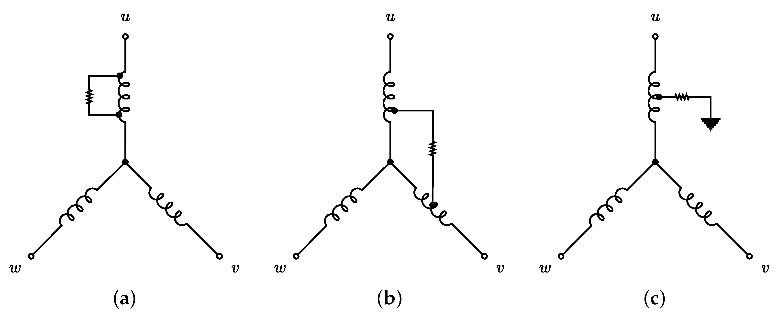
These faults can be schematized as depicted in Figure 1. The ITSC fault belongs to the turn-to-turn fault (see Figure 1a), the study object in this work. This fault can be provoked by the degradation of the conductor coating, which can be a product of the coating’s natural aging or, in most cases, of the rise in the stator temperature over the design parameters [31]. The circulation of high currents in the stator is the most common factor initiating this condition by the Joule effect, generally provoked by excessive mechanical loads during the start-up cycle. Also, if the fault is derived between stator phases, this fault is the named phase-to-phase fault (see Figure 1b), or if the fault is presented between the phase to chassis, it can create a derivation to the ground, generating the phase-to-ground fault (see Figure 1c). The origin could be the same regardless of the fault type.

On the other hand, the presence of ITSC in the stator creates a disturbance in the magnetic flux distribution in the air gap, inducing spurious currents that inject harmonics into the stator. These harmonic components $f_h$ can be located in the power spectral density as:

$$f_h=f_o\left[\frac{a}{p}(1-s)\pm b\right]$$

(1)

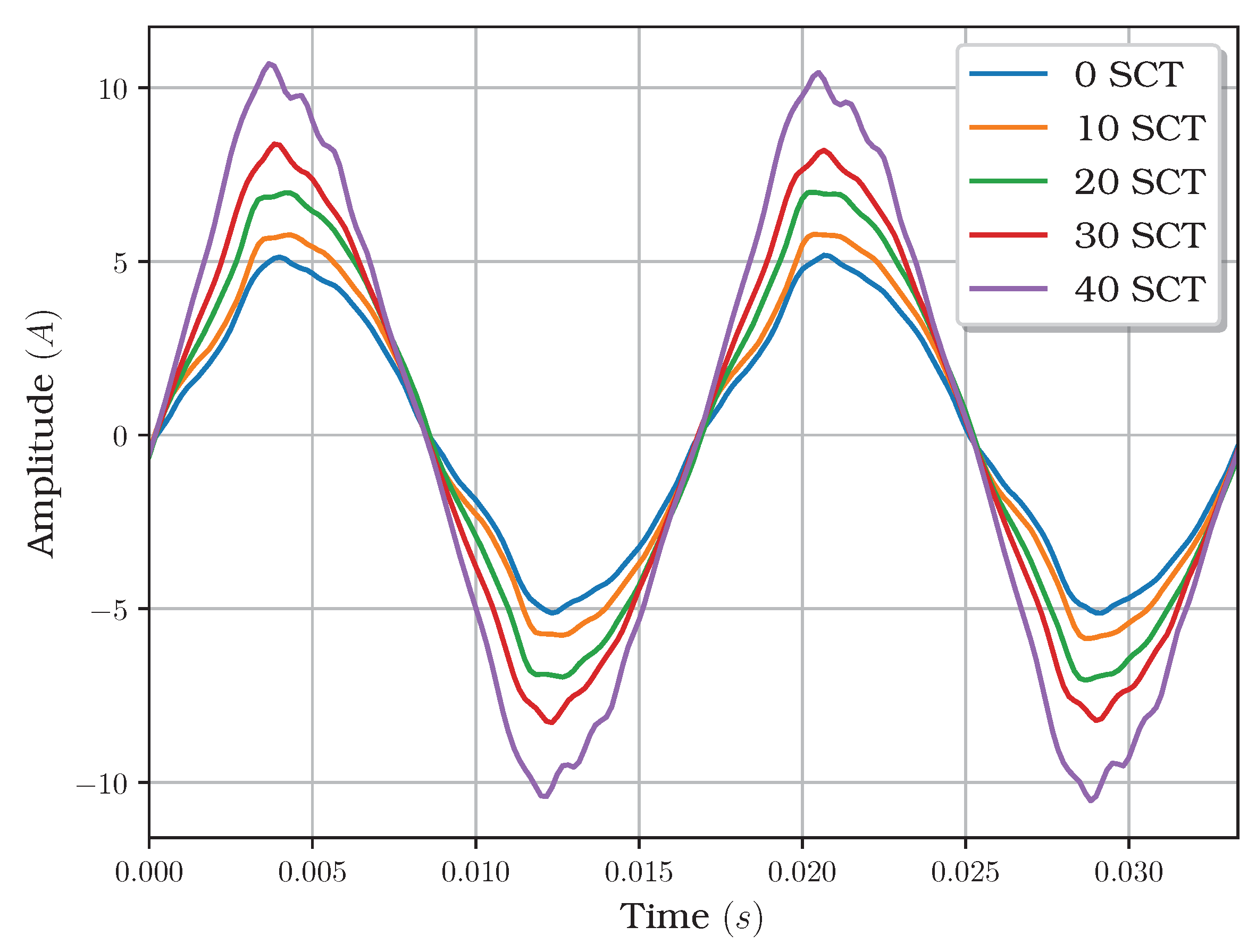
where $f_o$ is the fundamental frequency of the power source, a is the harmonic’s number (odd number), p is the pole pair, s is the slip, and b is an index. Since these faults can occur suddenly and gradually worsen over time, the fault presence is not evident until the machine breaks down. In this way, early detection of this fault is desirable to program corrective action on time. The harmonics induced by the presence of this fault in the current stator generate distortion in the shape of the sine wave provided by the electrical power source. 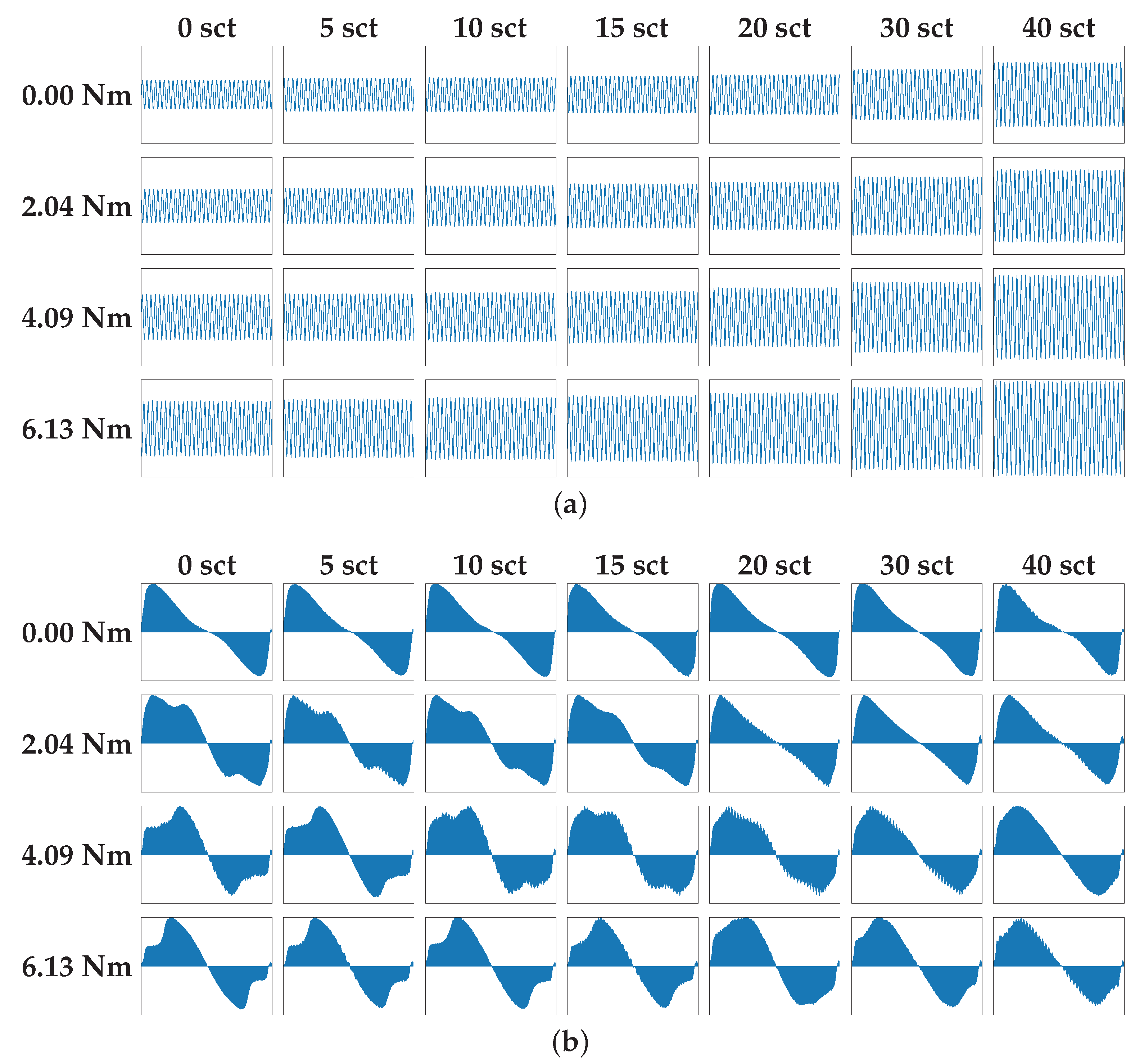As shown in Figure 2, the amplitude of the current stator signal, experimentally acquired as described in Section 2.3, appears to be increased by the level of damage, implying that it can be misleading since the increase in the mechanical load has a similar effect in the current stator, even in healthy conditions. These effects make the detection hard in the time domain.

However, if the signal is translated to another representation that allows information preservation, it could be enhanced to detect the ITSC harmonics signature efficiently. So, letting a set $X=[x_0,x_1,\dots ,x_{N-1}]\forall x_{N-1}\in \mathbb{R}$, the CDF $F_m$ is defined as (2):

$$F_m=P(X\le {\tilde{x}}_m)$$

(2)

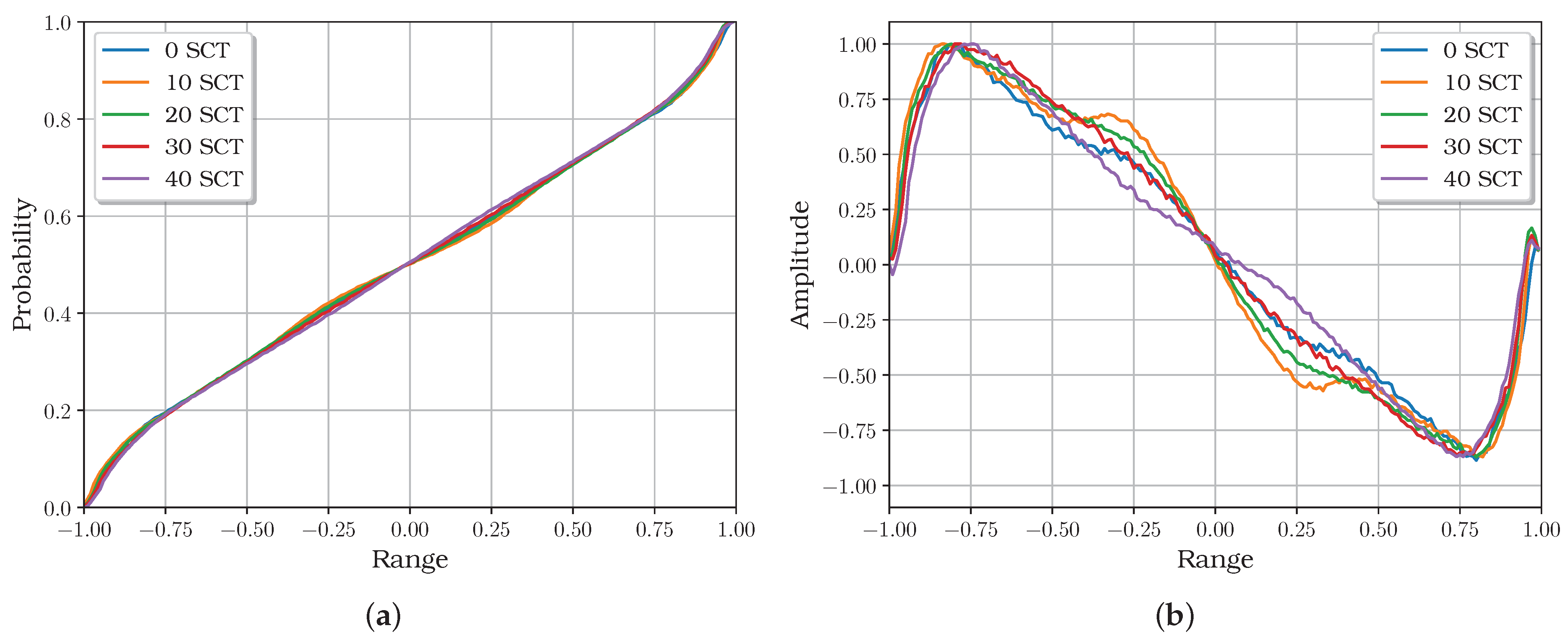
where $P(X\le {\tilde{x}}_m)$ is a value counter which satisfies the inequality condition $X\le {\tilde{x}}_m$ and ${\tilde{x}}_m\in \mathbb{R}$. Thus, the CDF of the current signals shows significant changes in shape (see Figure 3a) concerning the sine wave (see Figure 2), translating the information in a shorter data length, but does not reach enough separability between classes (damage stages at different mechanical loads).

To get through this, removing the typical linear incremental component could be a solution to highlight the features inserted by the different fault conditions, obtaining a kind of distorted one-cycle sine wave (see Figure 3b), in which the distortion could represent the signature of an existing fault. The processing of the CDF described above is presented as follows:

$$y_m=F_m-\frac{N}{M-1}m$$

(3)

where $y_m\in Y:Y\in {\mathbb{R}}^M$, M is the number of classes of the CDF, and $F_m$ is the m-th observation computed from (2). In this sense, the next challenge is developing or implementing a technique to detect small features in the modified CDF.

2.1. Convolutional Neural Network Overview

Proposed by LeCun et al. [32] in 1995, the CNN model is a kind of ANN with self-optimizable neurons and a more complex architecture, designed to emulate the visual cortex of the biological brain, be able to detect oriented edges and endpoint corners, and others.

Its architecture (see Figure 4) often consists of multiple layers; according to their function, these can be classified principally as three layer types [33]: convolutional, pooling, and fully connected. The convolutional layer applies the convolutional function to create feature maps to detect specific features. This layer can be denoted as in (4):

$$c_i=\sigma \left(\mathbf{w}\ast \mathbf{x}+\mathbf{b}\right)$$

(4)

where $\mathbf{w}$ is the filter or kernel, $\mathbf{x}$ is the image, $\mathbf{b}$ is the bias, $\sigma$ is an activation function, and ${\mathbf{c}}_i$ is the i-th feature map. Then, the convolutional layer is connected to the pooling layer, which applies down-sampling to reduce the data from the feature map, saving memory usage and training speed. The pooling layer can be represented as stated in (5):

$$p_i=\mathrm{pool}\left(c_i\right)$$

(5)

where $\mathrm{pool}\left(dot\right)$ is the pooling function and $p_i$ is the i-th network output. The fully connected layer consists of neurons connected between them, and its outputs are directly related to the predicted labels. This layer is usually located after a stack of convolutional layers, and it is represented as:

$$l=a\left(\mathbf{W}+\mathbf{b}\right)$$

(6)

where $\mathbf{W}$ is the weight matrix, $\mathbf{b}$ is the bias, and l is the predicted label. Due to their intrinsic features, these neural networks can classify wide data diversity. In addition, these architectures have been applied in areas such as computer vision, natural language processing, medical, industrial automation, and robotics, among others. Their versatility and ability to learn complex patterns make them a powerful tool in artificial intelligence.

Since their introduction in 1995, several models have been presented and included in the literature, solving and handling diverse problems and issues exposed by their predecessors. In particular, EfficientNetV2 is an innovative CNN introduced by Tan and Le in 2021 [34] as a new family of minor architecture, parameter efficiency, and faster training neural networks. This CNN solves the bottleneck presented by the predecessor, EfficientNet [35], proposing an improved progressive learning method and increasing the training speed to 11 times over the current architectures. The progressive learning method allows progressive changes in the image size and adaptive regularization adjustment during the training process, speeding up and making learning simple representations easier in the early stages.

The main improvement in this architecture over the last is the replacement of the MBConv with the novelty Fused-MBConv blocks (see Figure 5); in the first layers, both are combined, which results in an enriched search space, which increases speed and upholds accuracy. Finally, the authors recommend using the pre-trained model with the ImageNet data set to improve efficiency in future applications.

2.2. Methodology

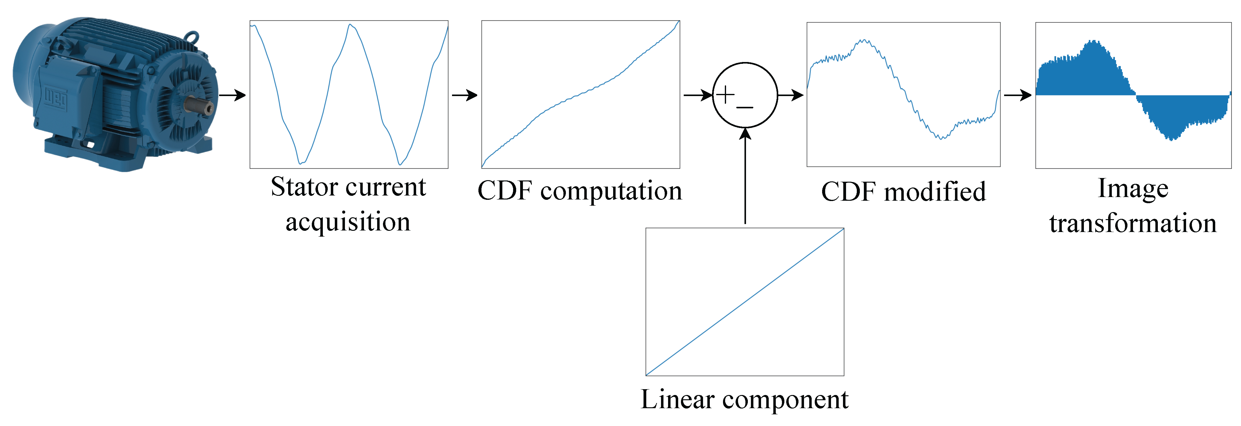
The proposed methodology is based on analyzing and processing the motor stator’s current signal using DL techniques to detect the ITSC fault in the early stages. The proposal is formed by two principal stages: pre-processing and detection. The steps to develop this are listed below.

2.2.1. Pre-Processing

• First, acquire the current signal from the motor stator of the IM to diagnose in a steady state to save N samples ($X\in {\mathbb{R}}^N$) for the following stages. Consider a normalization process of the signals between the $(-1,+1)$ range.
• Obtain the CDF of X with m classes ($F\in {\mathbb{R}}^M$) in concordance with (2).
• Delete the linear incremental component, applying (3), and obtain $Y\in {\mathbb{R}}^M$. Also, consider the normalization of Y in the $(-1,+1)$ range.
• Finally, generate an image of 3 × W × H dimension from Y, ensuring the area under the curve is shaded. Note that W is the wide and H is the height.

These steps are depicted in Figure 6.

2.2.2. Detection

The detection process is principally formed of two stages to apply the DL technique correctly: training and testing. The training process is developed once to give the CNN architecture the necessary information about the faults to detect (in this work), learning and applying them in the testing process. This last stage is used as required, performing the detection and finishing the methodology. The steps are listed as follows.

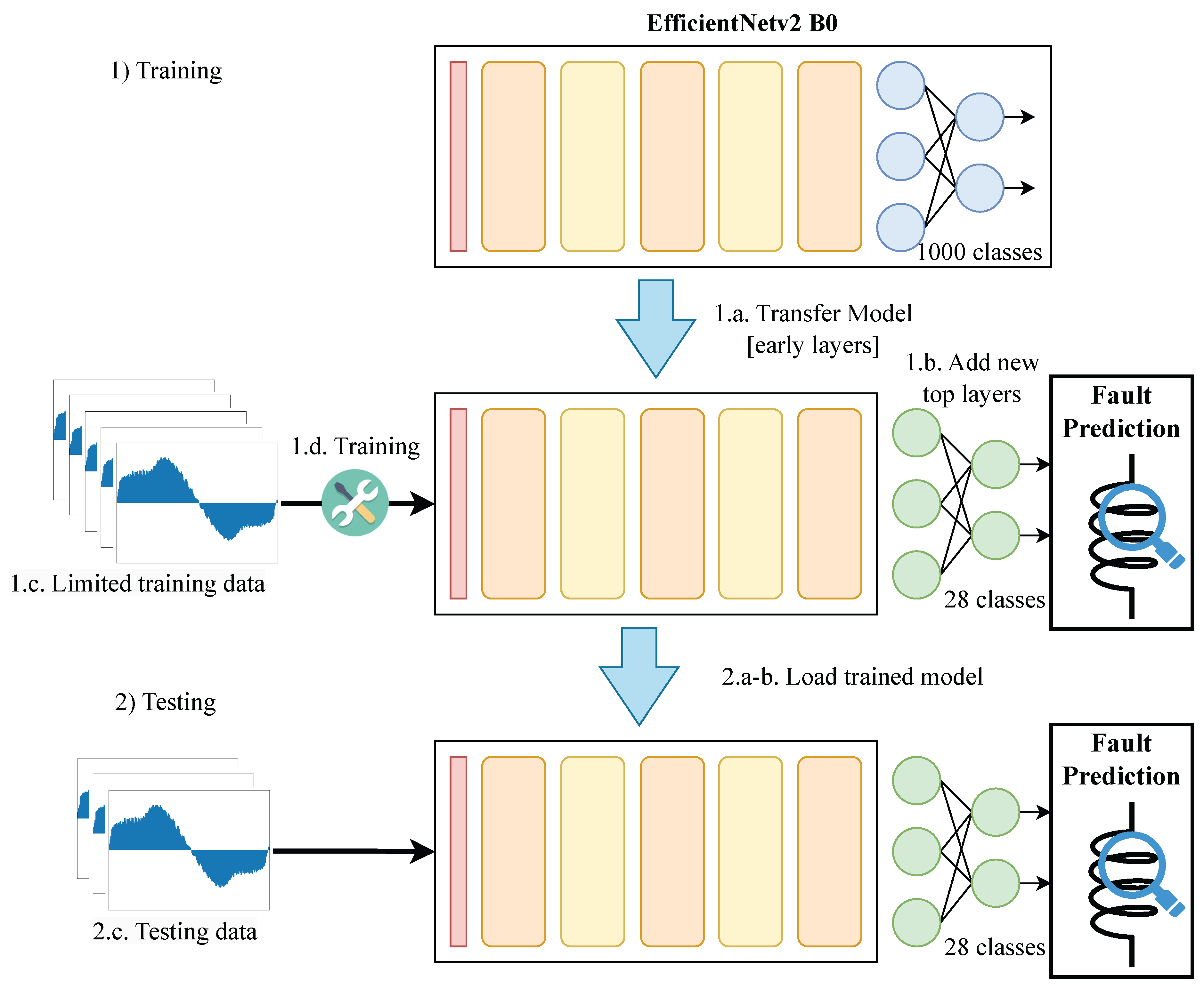
• Training process.

  (a)

  Initially, load the EfficientNetv2 model B0 version and realize the model transfer, preserving the early layers and omitting the top layers.

  (b)

  Then, construct and connect a new output layer in concordance with the desired output labels.

  (c)

  Next, prepare the data set with limited samples containing the processed CDF with different damage levels. Ensure the generated images (samples) and their labels are compatible with the CNN architecture’s input and output formats.

  (d)

  Launch a training process to adjust the weights with the prepared data set.

  (e)

  Last, when the training process is finished, save the adjusted weights for the testing process development.

• Testing process.

  (a)

  First, create a CNN model as steps a and b indicate in the training process.

  (b)

  After, load the obtained weights from the training process to the created model.

  (c)

  The image obtained from the modified CDF is introduced to the CNN, and the evaluation function is run.

  (d)

  Last, recover the results from the evaluation process to obtain the diagnosis.

The above-mentioned steps are illustrated in Figure 7.

2.3. Test Bench

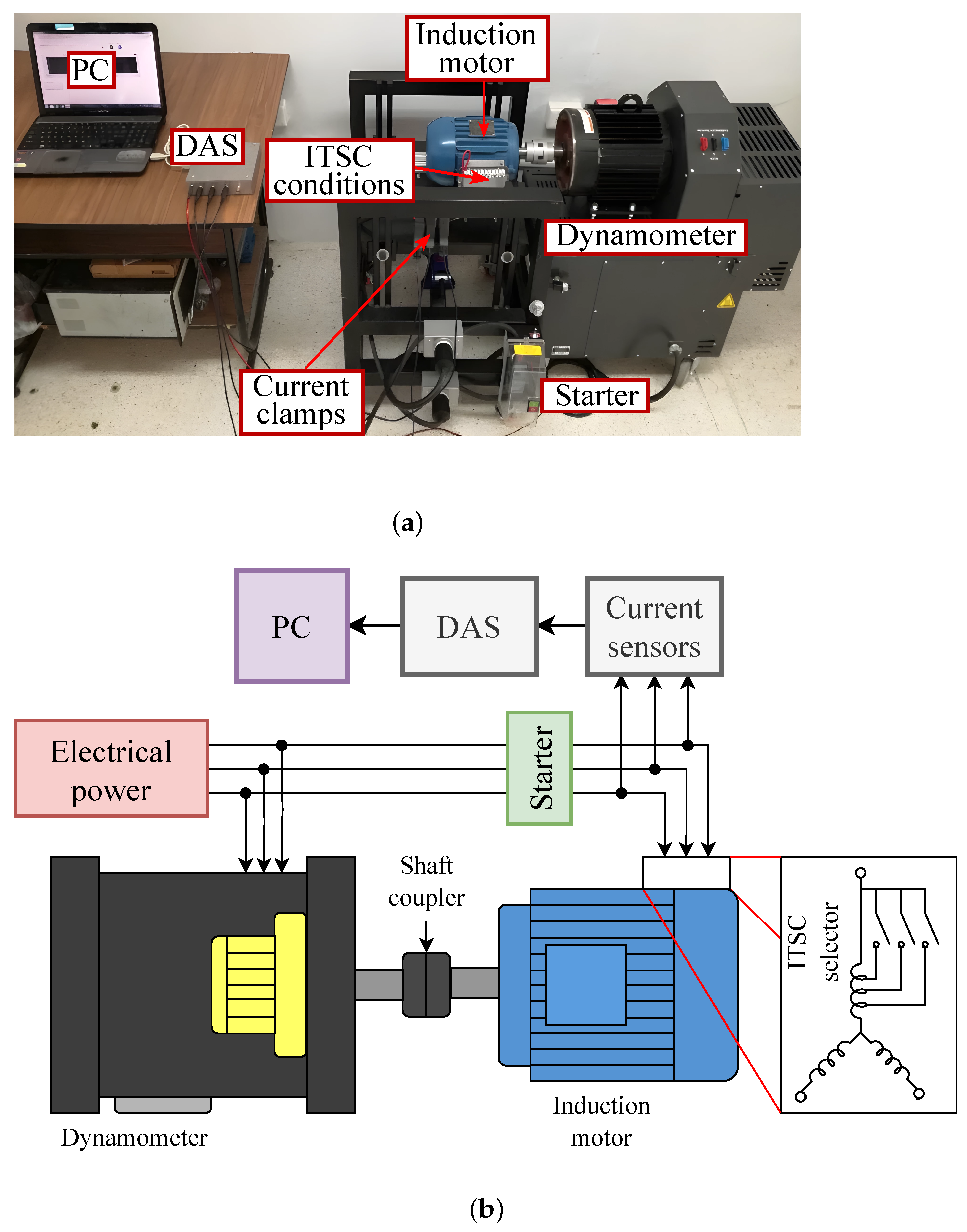
For validating the proposal efficiency, the IM used is the 218ET3EM145TW model of 2-Hp, 3-phase at 220 VCA @ 60 Hz with a stator of 141 turns per phase, from WEG coupled to a four-quadrant dynamometer model 8540 from Lab-Volt to control the mechanical load applied. The current signals from the stator phases were acquired by current clamps model i200s from Fluke, connected to a data acquisition system (DAS) model NI-USB-6211 from National Instruments. The DAS was connected and communicated to a personal computer (PC) to store the acquired signals. Also, a standard starter was installed to start and stop the motor. Figure 8 depicts the test bench used in this work.

Figure 7. Block diagram of the detection process.

Figure 7. Block diagram of the detection process.

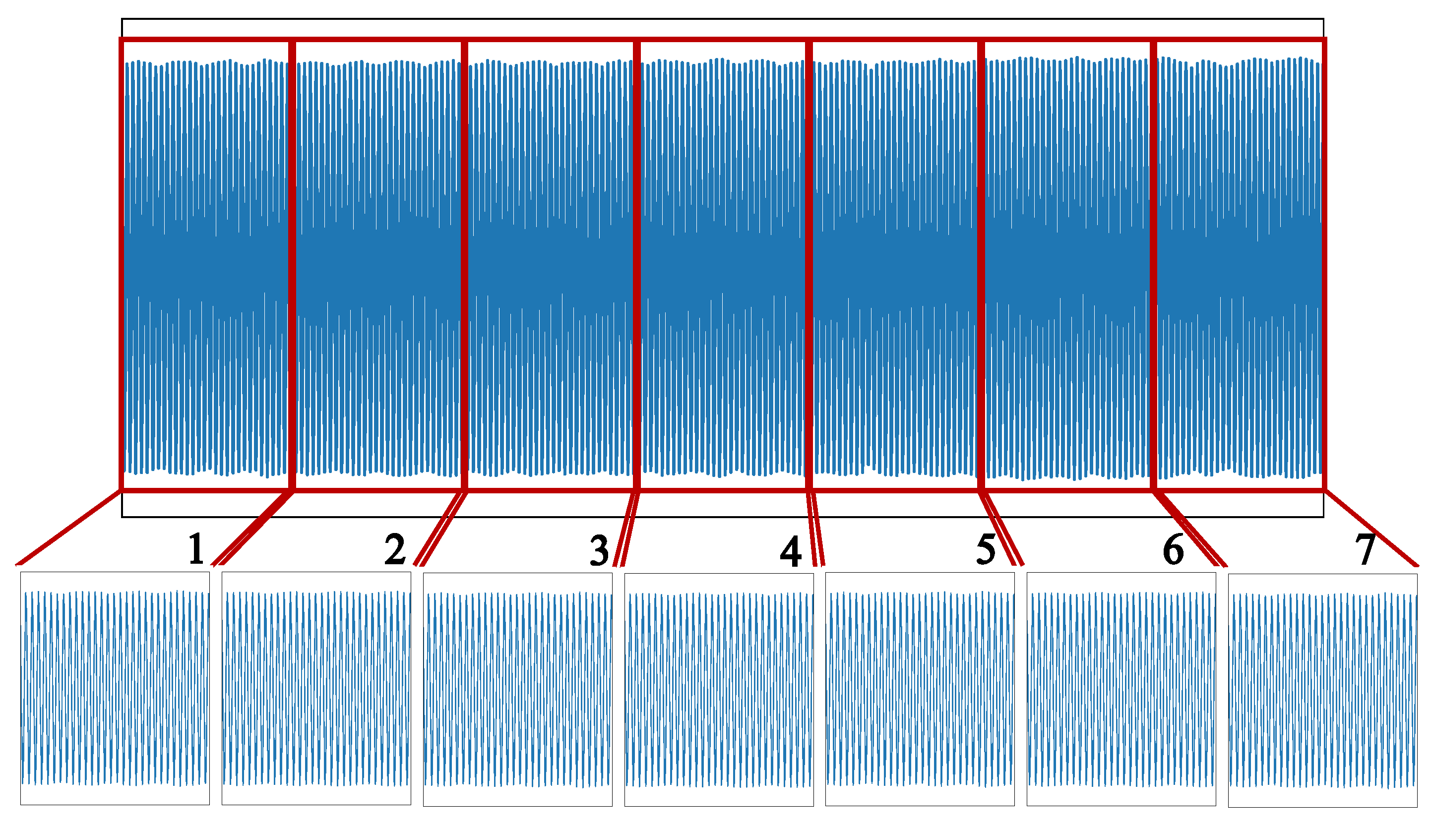
The stator motor was modified to create specific fault conditions in the IM, generating six ITSC fault conditions plus the healthy condition. The conditions with ITSC faults are 0, 5, 10, 15, 20, 30, and 40 short-circuited turns, with 0 SCTs being the healthy condition. The mechanical loads were simulated as fixed loads in 0%, 33.33%, 66.66%, and 100%, in concordance with the motor’s nominal power. These values were chosen to maintain homogeneity across the entire range of the motor’s nominal power. Regarding the above, 28 conditions were created: seven ITSC conditions at four different levels of mechanical load each. The current stator signals were acquired at a 6 kHz sampling rate in a steady state, and the motor was run at intervals of 3.5 s to avoid severe damage to the stator. Then, each acquired signal was segmented into seven parts to obtain seven testing signals of 0.5 s duration as depicted in Figure 9. All tests accumulated 1960 s and 11,760,000 signal points. It is important to say that the test bench’s configuration was prepared to be fed with the commercial electrical power grid in order to verify the feasibility of applying the proposed methodology under typical operating conditions.

3. Tests and Results

The current stator signals were acquired and pre-processed according to the earlier methodology. In this sense, a data set was created from the data generated during the acquisition stage. So, each fault condition was integrated by 140 signals of 0.5 s duration, which is enough acquisition time to detect the fault following preliminary testings. All signals were acquired from a motor fed by the commercial electrical power grid, and the application of fixed mechanical load levels and damage conditions was applied as specified in Section 2.3. This entails a data set of 3920 signal segments, converted to the modified CDFs with 200 classes and transformed into images of 3 × 224 × 224 pixels. The dimensions of the images were selected according to the input format of the selected CNN model to maintain its simplicity. In addition, the primary purpose of this representation is to reduce the number of points of the signals from 3000 to 200, comprising and preserving the information on the status of the stator motor, as well as less complex CNN applications.

Per each condition fault, 100 images were selected for the training process and 40 for the testing process; in other words, 71.4% of the data set (2800 images) was selected for training, a meager amount of data in contrast to the traditional training process in DL. Furthermore, the 5-fold cross-validation was applied [36] to avoid bias and explore the methodology’s effectiveness. This cross-validation consists of the random sample selection to be part of the training set, and the remaining is destined for the testing set. In this work, this process was repeated five times. Figure 10 graphically resumes the essence of this validation technique.

On another note, the necessity of using a CNN relies on the requirements of incipient fault detection. For example, this paper’s most challenging fault conditions are the 0, 5, 10, and 15 SCTs. Traditional classification often confuses these faults, especially at low or no mechanical loads, due to the difficulty of identifying the small features and differences related to them [19]. Figure 11 depicts an example with ten modified CDFs per the mentioned damage level. As can be shown, these lack remarkable differences. However, slight differences exist between positive and negative lobes, generally. This makes the identification possible.

In addition, the conversion to modified CDFs increases the differences between damage conditions over the time-domain signals. In Figure 12 note that time-domain signals highlight their amplitude, which can be easily mistaken with other damage conditions. However, modified CDFs show sensitivity lobes to the change in the damage and load conditions. In this way, the modified CDFs are preferred for fault detection in this work.

The implementation of the CNN models is described below. Due to its fast training process and relatively small architecture, the EfficienteNetv2 family model, specifically the most miniature model, the B0 version, was selected. This model has only six convolutional blocks and can be implemented with pre-trained ImageNet classification weights. As a result, the top layers must be replaced because, initially, the model could classify 1000 classes, and the purpose of the proposed methodology is to classify 28 classes only. In the case of the inputs, these were conserved as initially proposed by their authors: 3 × 224 × 224, to be compatible with RGB images. Finally, the model was constructed by using a similar top layers type, following the new number of classes in a categorical format and including a softmax activation in the last layer. The architecture summary is shown in

Table 1. Summary of implemented CNN architecture.

Layer	Output Shape	No. of Parameters	Basic Configuration
Input	(224, 224, 3)	0	–
EfficientNetv2-B0	(7, 7, 1280)	5,919,312	No top layers
Global Average Pooling 2D	(1280)	0	–
Dropout	(1280)	0	rate = 0.2
Dense	(28)	35,868	units = 28, activation = softmax

.

Three testing scenarios were established for the CNN effectiveness evaluation, described below. It is important to note that the CNN model only needs the RGB image and does not receive additional information, such as mechanical load.

3.1. Training with Randomly Initialized Weights

Implementing the architecture mentioned above, the training process was accomplished with a configuration of 30 epochs and a batch size of 5. The batch size was selected to minimize memory use and save the accuracy and speed of the process. In addition, the compiled model was developed with the Adamax optimizer, with categorical cross-entropy as the loss, and accuracy as the metric. All the trainable weights of the architecture were initialized randomly. Figure 13 shows the present training process. Note that it transfers only the convolutional blocks, and the replacement of the top layer is to be compatible with the number of classes in this work.

The results presented in

Table 2. Resume of results of training with randomly initialized weights.

Cross-Validation	Accuracy (%)		Loss (%)
	Train	Test	Train	Test
1	99.39	98.21	$2.147\times {10}^{-2}$	$8.228\times {10}^{-2}$
2	99.54	97.77	$1.940\times {10}^{-2}$	$1.069\times {10}^{-1}$
3	99.46	97.50	$2.012\times {10}^{-2}$	$1.178\times {10}^{-1}$
4	99.64	98.04	$1.604\times {10}^{-2}$	$6.515\times {10}^{-2}$
5	99.43	98.21	$1.865\times {10}^{-2}$	$6.679\times {10}^{-2}$
Average	99.49	97.95	$1.914\times {10}^{-2}$	$8.778\times {10}^{-2}$

demonstrate the high accuracy of the method, with the worst accuracy rate of 97.50% and the best at 98.21% and an average of 97.95%. This means that in the worst case, only 28 of 1120 images were wrongly classified, and in the best case, 20 images. This behavior is due mainly to the complex detection of the incipient’s damages, as exposed above. Also, the presented results emphasize the fast convergence of the CNN model since it only takes 30 epochs to reach the presented rates, a feature highlighted in this methodology and reported by their authors.

3.2. Training with Pre-Trained Weights

This test’s launch was conducted conclusively with the same configuration previously exposed; the difference relies on loading the ImageNet pre-trained weights to the selected CNN model (red dashed rectangles in Figure 14) as their authors recommend. In this manner, the information extracted earlier is readjusted, and the model can converge quickly and improve its performance. So, the model is compiled with the same number of epochs, batch size, optimizer, etc., to compare the rates it will reach. Results are resumed in

Table 3. Resume of results with ImageNet pre-trained weights.

Cross-Validation	Accuracy (%)		Loss (%)
	Train	Test	Train	Test
1	99.86	98.75	$5.644\times {10}^{-2}$	$4.588\times {10}^{-2}$
2	99.82	98.75	$7.189\times {10}^{-2}$	$5.934\times {10}^{-2}$
3	99.82	97.67	$6.737\times {10}^{-2}$	$10.960\times {10}^{-2}$
4	99.89	98.93	$6.778\times {10}^{-2}$	$4.837\times {10}^{-2}$
5	99.89	99.16	$3.849\times {10}^{-2}$	$2.998\times {10}^{-2}$
Average	99.86	98.65	$6.039\times {10}^{-3}$	$5.863\times {10}^{-2}$

.

As expected, this process enhanced the training process, improving the accuracy rate by 0.7% over the last average and covering up to 99.16% in the best of cases, failing nine images in the correct class.

3.3. Transfer Learning and Fine-Tuning

TL is a powerful technique used in CNN as an alternative when access to a data set with many samples is unavailable. This technique uses pre-trained CNN, and the information learned will be applied to new applications. This implies transferring the architecture without the top layer and replacing it with another in concordance with the application. The development of TL in this work used the application of the typical workflow, described as follows.

• A new architecture implementation shown in Table 1 is performed and ensures the loading of pre-trained weights. The transferred layer is frozen to avoid re-adjusting their weights in the new training process. Therefore, only the weights of the top layer will be trained.
• Then, the model compilation is performed with the configuration applied in the latest procedures, ensuring the base model is instantiated in inference mode.
• So, the training process is run with 20 epochs and a batch size of 5.

Continuing development of the FT technique is recommended if the scores obtained are not as high as expected. In the case of this work, the score obtained by TL is about 90%, so the FT is applied, following the next steps.

• Unfreeze the layers of the base model.
• Recompile the model as performed previously and set a very low learning rate to ensure the weights are updated slowly and lightly (fine-tuning). In this work, a rate of $1\times {10}^{-5}$ was configured.
• Run the re-training process. The configuration of the training process for fine-tuning is 20 epochs and a batch size of 5.

A simplified schematic of this process is depicted in Figure 15.

The results obtained from the TL and FT development have scant differences (see

Table 4. Resume of results with transfer learning and fine-tuning technique.

Cross-Validation	Accuracy (%)		Loss (%)
	Train	Test	Train	Test
1	98.75	98.48	$5.275\times {10}^{-2}$	$5.454\times {10}^{-2}$
2	98.82	96.87	$4.428\times {10}^{-2}$	$8.990\times {10}^{-2}$
3	99.11	97.50	$4.195\times {10}^{-2}$	$11.757\times {10}^{-2}$
4	98.82	97.32	$4.869\times {10}^{-2}$	$7.838\times {10}^{-2}$
5	98.75	97.14	$4.856\times {10}^{-2}$	$8.546\times {10}^{-2}$
Average	98.85	97.46	$4.725\times {10}^{-3}$	$8.517\times {10}^{-2}$

). While it appears to be the lowest testing rate, the accuracies differ by less than 2%. So, this approach could be an alternative because one of the main assumptions of this technique is fast convergence.

Table 5. Average times of training approaches.

Approach	Average Time (s)
Randomly initialized weights	1379
ImageNet pre-trained weights	1292
TL and FT	316 and 728

presents the average times of each training process.

On the other hand, the testing results ensure that the detection process takes 0.107 s (including signal-to-image conversion) once the signal is acquired (0.5 s). Thus, the method can provide two fault diagnoses per second or one diagnosis in 0.607 s. It is important to note that the training process is developed once and generally accomplished offline, allowing the detection process time to remain unaffected.

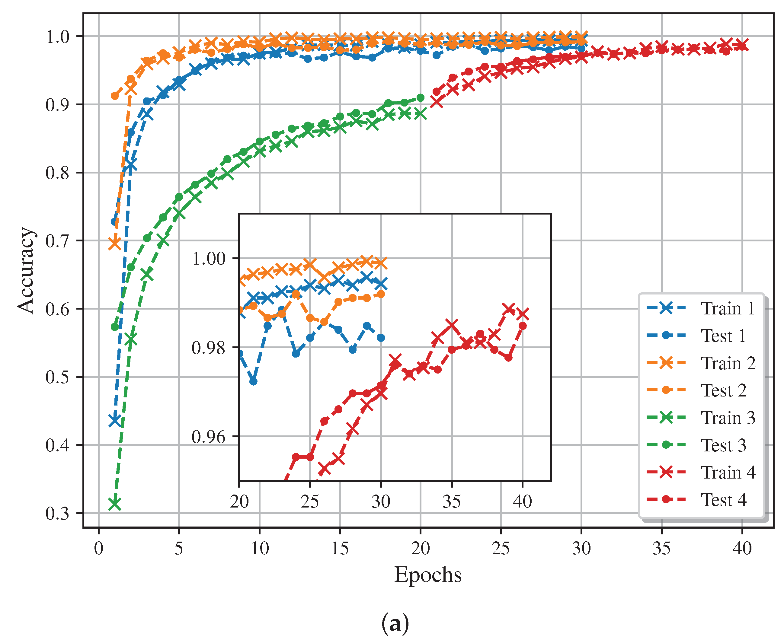
Figure 16 shows the accuracy and loss results of the CNN training process with the different applied training approaches. Note the fast convergence and the high accuracy and low loss rate reached. Also, the TL and FT techniques use more epochs, but these are executed faster than the others.

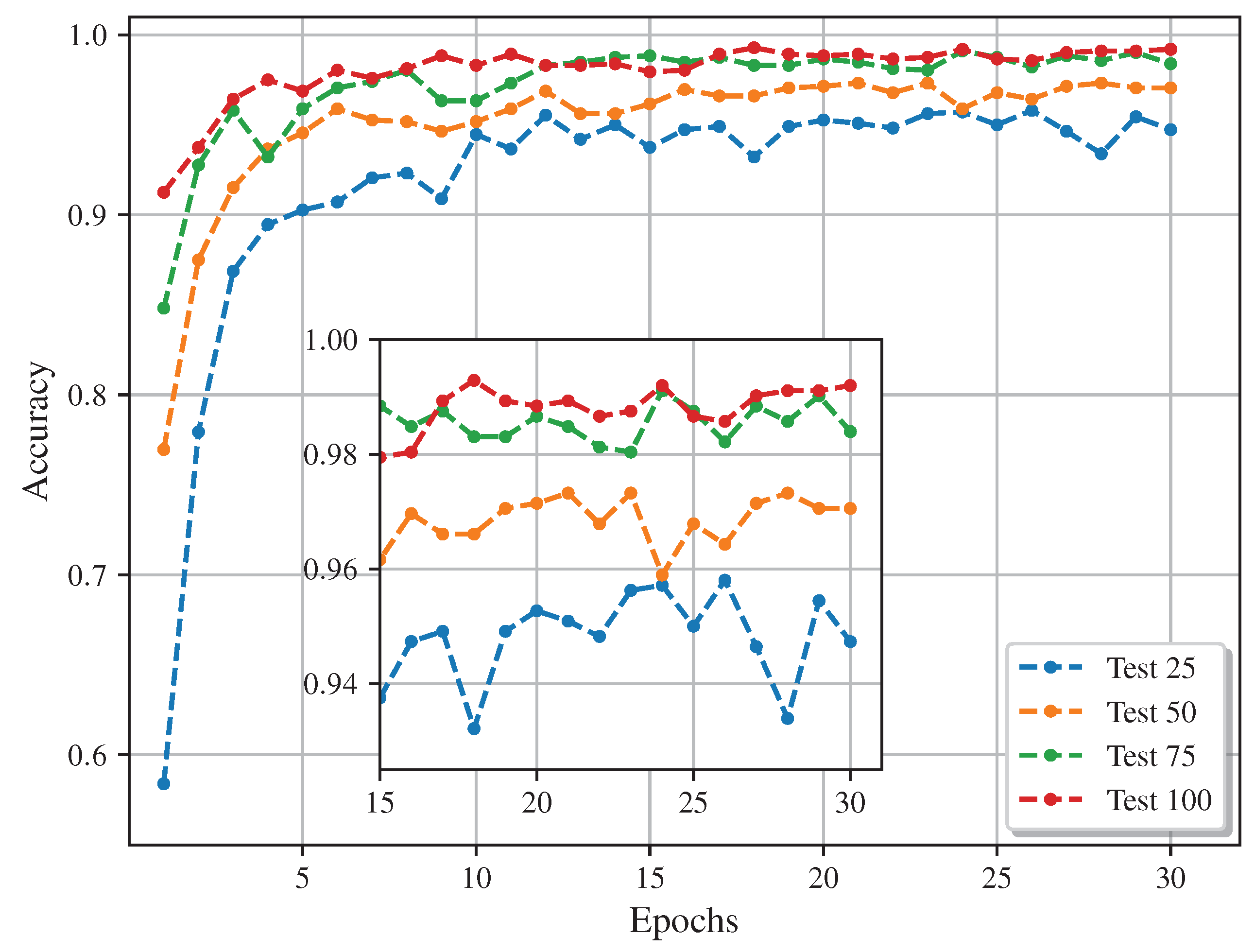
In addition, testing using 25, 50, and 75 images per condition (700, 1400, and 2100 images in total, respectively) for the training process was developed, as Section 3.2 specifies, to explore the effectiveness with smaller data set applications. The final accuracy of the tests was 94.73, 97.05, and 98.39%, respectively. Compared to the best result with 100 images per condition of 99.16% (see Table 3), the higher the data set, the higher the accuracy rate. These comparisons are depicted in Figure 17, where the high compatibility of the selected CNN model and the modified CDFs and the high effectiveness of the model with smaller data sets are also demonstrated since a high accuracy rate can be obtained (over 90%) even in a data set with a significant lack of samples.

The tests were developed in Python version 3.11, using Tensorflow version 2.15 and the Keras version 2.10 library. The used hardware was a Dell G15 with an Intel Core i7-13650HX, 16 GB of RAM, and an NVIDIA GeForce RTX 4060 GPU board with 8 GB of dedicated RAM. The configuration of TensorFlow and Keras for GPU hardware usage was accomplished according to the published procedure on the TensorFlow web page [37].

4. Discussion

The results of implementing the proposed methodology indicate that it successfully detected the 28 ITSC conditions, regardless of the applied mechanical load. Thus, the reached accuracy rate of 98.75–99.16% and an average of 98.65% proves the effectiveness of the methodology for detecting incipient damage up to 5 SCT as minimal, damage that represents 3.5% of the total turns in the motor stator. As planned, loading the ImageNet pre-trained weights shows the best results, one of the most highlighted model features reported in the literature [34]. Conversely, the training process with weights randomly initialized retrieved a high accuracy rate of 97.50–98.27% and an average of 97.95%, much better than expected. This process typically uses a high amount of data and epochs to reach a high accuracy rate, contrasting with the model used in this work under previously expressed conditions. Also, TL and FT promised great potential in this application; concerning the development, this approach was a better fit for this application. However, it gave the lowest rates of 97.14–98.48% and an average of 97.46% in this work. Despite that, the results are comparable with those previously discussed, and it is an alternative to small data sets. In addition, Figure 16 presents an exceptional performance of the CNN model. However, the graph suggests stopping the training at 20 epochs since the changes are insignificant (less than 1%) for the two first approaches. On another note, the TL and FT techniques could improve the results if the epochs number is increased; however, this can be unproductive since reaching overfitting is possible.

Table 6. Comparison of the proposed methodology with similar techniques in the literature.

Work	Technique	Mechanical Load (%)	Severities	Accuracy (%)
[7]	(a) Statistical features from a quaternion analysis (b) Decision tree	No load	0, 6,12, 18, and 24 SCTs	99
[10]	(a) Discrete Wavelet Coefficients (b) L1 and L2 norms (c) ANN	0, 25, 50, 75, 100, and 125	0, 1, 3, 5, 7, 10, 13, 15, 17, 20, 23, 25, 35, 45, 55, 65, 80, and 90 SCTs	95.29
[11]	(a) Empirical wavelet transform (b) statistical features (c) Linear discriminant analysis (d) Self-Organizing Neural Network	20	0, 2. 4, and 6 SCTs	100
[23]	(a) Negative sequence current analysis (b) Probabilistic Neural Network	No specified	0, 1, 2, 3, 4, 5, 6, 7, 8, 9, and 10 SCTs	90
[24]	(a) Statistical features from time-based from torque (b) Magnitude of spectra estimation (c) Multi-layer feed-forward neural network	0, 10, 20, 30, 40, 50, 60, 70, 80, 90, and 100	0, 1.9, 3.9, 7.9, 11.9, 15.8, 19.8, 23.8, and 27.7%	88–99
[25]	(a) Hilbert transform (b) Variational mode decomposition (c) Correlation (d) SqueezeNet model and TL	0, 30, and 50	5, 7, 13, 15, and 20 SCTs	99.8
[26]	(a) Empirical mode decomposition (b) Statistical features (c) Long Short-Term Memory.	No specified	0, 1, 2, 5, 7, and 15 SCTs	95
This work	(a) CDFs obtention from current signals (b) EfficientNetv2-B0 model CNN	0, 33.33, 66.66, and 100	0, 5, 10, 15, 20, 30, and 40 SCTs	98.75–99.16

presents a comparative analysis of the results obtained by the proposed method alongside the latest research utilizing similar techniques presented in the literature for detecting ITSCs in IM. Specifically, it details the techniques or methods employed in each study, the mechanical load conditions, fault severity levels, and the efficacy reached in assessing the IM condition. According to this table, it is possible to note that the ANNs at different levels of complexity are applied to the incipient ITSC fault diagnosis. While other techniques present effectiveness in lower levels of ITSC damage with diverse levels of mechanical load [10,24,25] or under a single or no mechanical load [7,11,23,26], they apply elaborated preprocessing stages, which increase their computational complexity and could limit their implementation in an industrial process. In this regard, for example, Guedidi et al. [25] investigate a SqueezeNet model, a lightweight CNN network, for detecting ITSCs in an IM, reaching high accuracy rate. Their proposal relies on the use of several signal processing techniques (e.g., Hilbert transform, variational mode decomposition, and correlation) prior to introducing the identified features to SqueezeNet, thereby increasing its computational resources. In addition, a more significant amount of data is used for the training process in all works of Table 6. In this way, the proposed methodology reaches accuracies that can compete and, in some cases, improve that presented in the literature, being that its main features or advantages are (1) a low computational complexity because it only uses a preprocessing stage and (2) that it can be employed regardless of the mechanical load since the lightweight CNN is trained from different load levels and does not need additional information or adjustments to accomplish the diagnosis. Although promising results have been achieved by the proposal, further research is necessary in order to enhance its robustness. In this regard, it is important to continue exploring other case studies that address various scenarios: (1) a wider range of faults, e.g., bearing damage, broken rotor bars, among others, (2) time-varying regimens, i.e., those produced by a frequency variator, and perturbations in the electric network or noise, (3) a greater variety of load levels and dynamic profiles of mechanical load, and (4) exploring other lightweight CNN networks, such as WearNet, ShuffleNet, RasNet, among others [38]. Calibrating the proposal under these circumstances will enable the investigation of a wider range of scenarios. At present, the performance of the proposed method may be compromised in such situations.

5. Conclusions

This paper presented a novel methodology for ITSC fault detection in IM based on DL and the development of a training process with a small data set. The CDF of stator current signals was obtained, and the typical linear component was subtracted to highlight the fault signatures. So, these modified CDFs were converted to images to apply DL techniques using the EfficientNetv2-B0 model, whose compact architecture and fast training process are highlighted, reaching an accuracy rate of up to 99.16%. Also, a re-training process was developed with barely 2800 images for 28 fault conditions with barely 30 epochs. This allowed the effective detection of the fault up to 5 SCTs regardless of the applied mechanical load. That way, it is demonstrated the detection of incipient ITSC with modified CDFs and the versatility of the followed workflow, solving the problem of limited data sets, an important constraint in this area. This opens the possibility of expanding this methodology to other areas of fault detection in IMs.

The work will expand to detect minor faults over 5 SCTs in the future, applying TL and FT to explore the technique’s performance, including additional operating conditions and motor configurations. Also, combined fault detection will be explored. These goals will contribute to developing more robust methods that can be integrated into online and reliable fault tolerant-control strategies.