Fault Diagnosis in Drones via Multiverse Augmented Extreme Recurrent Expansion of Acoustic Emissions with Uncertainty Bayesian Optimisation

Abstract

Drones are a promising technology performing various functions, ranging from aerial photography to emergency response, requiring swift fault diagnosis methods to sustain operational continuity and minimise downtime. This optimises resources, reduces maintenance costs, and boosts mission success rates. Among these methods, traditional approaches such as visual inspection or manual testing have long been utilised. However, in recent years, data representation methods, such as deep learning systems, have achieved significant success. These methods learn patterns and relationships, enhancing fault diagnosis, but also face challenges with data complexity, uncertainties, and modelling complexities. This paper tackles these specific challenges by introducing an efficient representation learning method denoted Multiverse Augmented Recurrent Expansion (MVA-REX), allowing for an iterative understanding of both learning representations and model behaviours and gaining a better understanding of data dependencies. Additionally, this approach involves Uncertainty Bayesian Optimisation (UBO) under Extreme Learning Machine (ELM), a lighter neural network training tool, to tackle both uncertainties in data and reduce modelling complexities. Three main realistic datasets recorded based on acoustic emissions are involved in tackling propeller and motor failures in drones under realistic conditions. The UBO-MVA Extreme REX (UBO-MVA-EREX) is evaluated under many, error metrics, confusion matrix metrics, computational cost metrics, and uncertainty quantification based on both confidence and prediction interval features. Application compared to the well-known long-short term memory (LSTM), under Bayesian optimisation of the approximation error, demonstrates performances, certainty, and cost efficiency of the proposed scheme. More specifically, the accuracy obtained by UBO-MVA-EREX, ~0.9960, exceeds the accuracy of LSTM, ~0.9158, by ~8.75%. Besides, the search time for UBO-MVA-EREX is ~0.0912 s, which is ~98.15% faster than LSTM, ~4.9287 s, making it highly applicable for such challenging tasks of fault diagnosis-based acoustic emission signals of drones.

1. Introduction

Drones have emerged as a pivotal technology in modern applications, encompassing a wide range of sectors from aerial photography and agricultural monitoring to critical roles in emergency response and logistics [1,2]. Consequently, the reliability and efficiency of drone operations are paramount, particularly in high-stakes environments [3,4]. Ensuring continuous operational integrity requires robust fault diagnosis systems that can promptly identify and address issues, thereby minimising downtime and optimising resource allocation [5,6]. The significance of effective fault diagnosis extends beyond operational efficiency to include substantial cost savings in maintenance and heightened mission success rates. Traditional fault diagnosis methods, such as visual inspections and manual testing, have long been the cornerstone of drone maintenance. These methods involve human operators examining the physical components of drones for signs of wear and tear, damage, or malfunction. Manual testing typically includes routine checks and tests to ensure all systems are functioning correctly. While these approaches have been reliable and effective to some extent, they are often time-consuming, and labour-intensive, and may not detect subtle or emerging issues that could lead to significant problems if left unaddressed [7]. Accordingly, these approaches often fall short in the face of modern technological demands, particularly when dealing with the increasing complexity and volume of data generated by advanced drone systems [8]. The advent of data-driven methods, leveraging machine learning, deep learning, and artificial intelligence in general, offers a transformative approach to fault diagnosis [9]. These methods can learn complex patterns and relationships within data, facilitating more accurate and timelier fault detection [10].

Despite their promise, these techniques are not without challenges. In fact, analyzing recent state-of-the-art works reveals these important challenges and gaps. Some significant contributions have been made in this field, and this paper highlights the most recent ones for illustration. For instance, the authors in [11] discuss fault experiments conducted on the stator, rotor, and bearing components of quadrotor drone DC brushless motors, leveraging their structural and operational characteristics. They introduced a hybrid mapping-based neural network model, with its main component being a convolutional neural network, to address the complexities of drone fault diagnosis. This approach used the current signal as the diagnostic input, addressing challenges in sensor installation and data acquisition. The hybrid model aims to achieve enhanced feature space representation and accurate learning. The work in [12] presents a method for monitoring the vibration signals of drones using a wavelet scattering long short-term memory autoencoder network to detect propeller blade malfunctions. Wavelets help reduce data uncertainties and complexity through their ability to provide robust representations and effective denoising, aiding in the accurate detection of anomalies. The study in [13] investigates methods for fault diagnosis in drones by introducing semi-supervised models. A mixture of convolutional learning models, a variational autoencoder, and three popular generative adversarial models are utilised. Data preprocessing involved various scaling methods, and hyperparameters were optimised using Bayesian methods. The fault diagnosis models employ a two-step approach for binary classification and likelihood ranking to detect the anomaly source. The proposed scheme was validated with real-world flight data, revealing major faults and identifying specific abnormal channels, which has implications for future UAV autonomy research. In [14], authors proposed a small-sample transfer learning fault diagnosis approach to extract meaningful fault patterns from drone engines, utilising deep learning. This approach involves converting vibration signals into two-dimensional time-frequency maps using multiple simultaneous squeezing S-transforms, which reduces the randomness of extracted features. Subsequently, a transfer diagnosis strategy is introduced by fine-tuning a ResNet-18 [15] convolutional neural network.

Despite these significant contributions and advancements, there is still room for improvement as certain gaps remain. For instance, while the models in Ref. [11] and Ref. [14] aimed to address the challenge of small sample sizes to mitigate uncertainty in fault diagnosis, they lack a specific straightforward examination or quantification of uncertainty in predictions. Additionally, the data, which typically exhibit complexity in real-world scenarios, were processed directly with a specific mapping, neglecting preprocessing steps to address uncertainties, outliers, noise, and other potential sources of data malfunctions. In [12], although wavelets offer more meaningful data representation, they are not outlier-specific, leaving room for measurement uncertainties. This issue persists due to the lack of advanced data preprocessing and specific uncertainty-aware learning methodologies. Furthermore, the authors in [13] effectively address the complexities in data associated with such problems; however, there is still room for improvement in quantifying uncertainty within the learning process itself.

Overall, clear research gaps in data preprocessing and uncertainty quantification highlight opportunities for advancements in drone fault diagnosis using advanced representation learning algorithms. Not to mention, the complexities in deep learning architecture itself lead to significant computational costs. Accordingly, several key challenges underscore the necessity for innovation in drone fault diagnosis. (i) The multifaceted nature of data, poses significant hurdles in extracting meaningful insights. Additionally, (ii) the variability, noise, and outliers in data necessitate robust methods for preprocessing, quantifying, and managing uncertainty, ensuring reliable fault predictions. Furthermore, (iii) developing models that are both accurate and computationally efficient remains a critical challenge, particularly when dealing with real-time fault diagnosis. As highlighted in [16], domain-specific challenges in drone diagnosis, including variability, noise, and outliers, stem from the inherent complexities of drone operations and the environments in which they operate. Variability arises from the dynamic and unpredictable nature of drone operations, such as varying environmental conditions (weather, temperature, and humidity) and diverse operational scenarios (flight paths and payloads). Noise is a significant factor due to the high-speed rotation of motors and propellers, combined with additional interference from environmental elements like wind and nearby obstacles, which complicates the task of distinguishing between normal operational noise and fault signals. Outliers are caused by rare but impactful events, such as hard landings or unexpected collisions, which produce unique acoustic signatures essential for accurate diagnosis but are challenging to predict and capture consistently. Sensor anomalies, resulting from electromagnetic interference or physical damage, also contribute to outliers that require careful management. By addressing these domain-specific issues and understanding their underlying causes, we aim to enhance the robustness and accuracy of data-driven methods for drone diagnosis [17,18].

To address these challenges, this paper introduces a novel methodology to enhance fault diagnosis in drones through an innovative approach termed UBO-MVA-EREX. This approach facilitates a deeper iterative understanding of both learning representations and model behaviours, effectively capturing data dependencies. In conjunction, it employs UBO integrated with ELM to mitigate data uncertainties and reduce modelling complexities. The core contributions of our research include the following:

• Use of acoustic emission signals: In this work, acoustic emission data is utilised as it allows capturing waves from localised energy releases within materials. It enables structural health monitoring by detecting cracks, material fatigue, and impact damage. It also monitors motor and propeller conditions, identifying bearing faults and propeller imbalances through high-frequency signals and abnormal acoustic patterns. Additionally, this data helps in flight condition monitoring by analyzing aerodynamic noise and environmental interference. The primary diagnosis tasks include fault detection and localisation, condition assessment, and performance optimisation [19].
• Data preprocessing: A well-designed pipeline is implemented to handle feature extraction, scaling, denoising, outlier removal, and data balancing. This ensures that the data is clean, consistent, and suitable for accurate and reliable analysis or modelling.
• Multiverse augmented recurrent expansion: This representation learning framework iteratively enhances the understanding of data and model behaviours. The model is based on multiverse recurrent expansion theories, with Inputs, Mappings, and Estimated Targets, denoted as IMTs, undergoing multiple enhancements, including neuron pruning [20], dropout [21], and principal component analysis (PCA) dimensionality reduction [22]. Additionally, IMT augmentation via polynomial mappings is further studied to improve representations [23].
• Integration with ELM: Unlike previous multiverse representations, the current version utilises a lighter and faster ELM for computational efficiency [24,25,26]. This integration demonstrates significant improvements in handling complex acoustic emission data.
• Uncertainty Bayesian optimisation: To mitigate uncertainties in measurements, we integrate a method for optimisng model parameters under an uncertainty quantification objective function [27]. This enhances the robustness and reliability of fault diagnosis. The objective function incorporates features from both confidence intervals and prediction intervals, such as coverage and width, to ensure comprehensive uncertainty quantification and improved model performance [28].
• Evaluation metrics: The model’s evaluation employs a comprehensive set of metrics, including error metrics (Root Mean Square Error (RMSE), Mean Absolute Error (MAE), Mean Squared Error (MSE), and the coefficient of determination (R²)), confusion matrix classification metrics (accuracy, precision, F1 score, recall), uncertainty quantification metrics (interval width), and computational time [29,30]. The novel integration of these diverse metrics, particularly the use of ordinal coding instead of traditional hotkey encoding for better uncertainty quantification, provides a more robust and nuanced evaluation framework. This combination of metrics has not been previously applied in this specific context, making it a unique contribution to the field.
• Evaluation datasets: The proposed UBO-MVA-REX framework is uniquely assessed using three realistic datasets specifically focused on the propeller and motor failures in drones [31]. This targeted evaluation using these specific datasets, combined with our novel methodology, represents a new approach not previously explored. Our results demonstrate that UBO-MVA-REX outperforms basic ELM and other deep learning models in terms of performance, certainty, and cost efficiency. The innovative use of these datasets with our comprehensive evaluation metrics highlights the originality and effectiveness of our approach to diagnosing drone failures.

This integrated methodology combines robust data preprocessing, advanced representation learning, efficient modelling, and uncertainty quantification to significantly improve fault diagnosis in drones. The closest work in this case is the one presented in previous work in [32]. However, it should be noted that these current contributions are not an extended version, they are completely new contributions while previous works only used one subset and different philosophy of deep learning and recurrent expansion and did not target uncertainty concepts.

The remainder of this paper is organised as follows: Section 2 provides a detailed description of the materials used in this work, including the main features of the discussed drones’ types, methods for failure injection, data generation, and proposed data preprocessing methodology. Section 3 explains the UBO-MVA-REX methodology in detail, covering the main learning rules, representation enhancement techniques, uncertainty quantification methodology and its objective function. Section 4 presents the results of the study and discusses their implications. Finally, Section 5 summarises the key findings and opportunities of this research.

2. Materials

This section provides a comprehensive overview of the materials used in this work. It details the main features of drone models utilised, including their specifications and variations. Additionally, it describes methods employed for inducing failures, the data generation process, and subsequent data processing methodology. This section lays the foundation for understanding the experimental setup and the procedures followed to obtain and prepare the dataset for analysis.

2.1. Dataset Generation Methodology

The dataset used in this study is obtained from a prior investigation [31]. The scientists employed three distinct drone models in the data generation procedure in this investigation. The drone types shown in Figure 1 are identified as A, B, and C. More precisely, Type A refers to Holy Stone HS720, Type B refers to MJX Bugs 12 EIS, and Type C refers to ZLRC SG906 Pro2. These drones vary in multiple ways, such as frame dimensions, mass, motor characteristics, and propeller measurements.

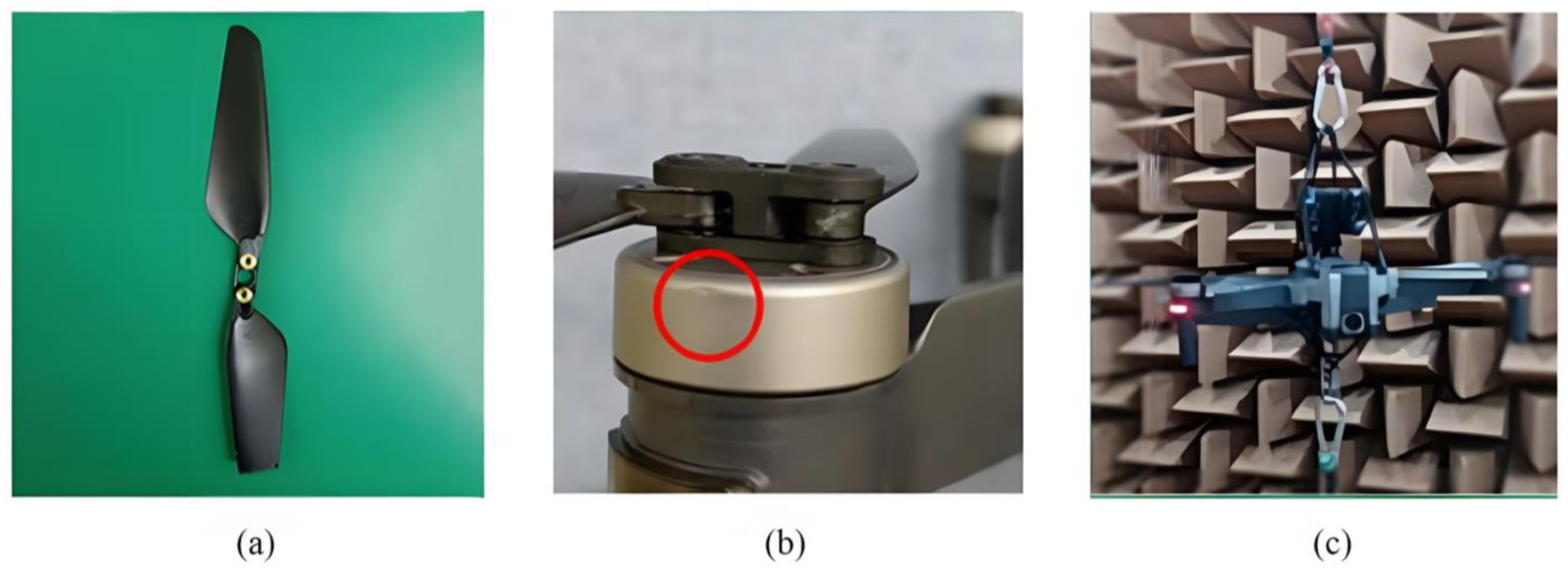
To create a faulty drone dataset, two common types of damage were introduced to normal drones: Propeller Cutting (PC) and motor cap denting, identified as the main Motor Fault (MF). In the PC scenario, approximately 10% of a single propeller was removed, resulting in a loss of balance and abnormal vibrations. For MF, a vice was used to crush the cap that supports the rotor and protects the coil, thereby increasing friction and hindering smooth motor rotation. Figure 2a,b illustrate both types of faults, PC and MF, respectively, to provide a visual reference for these damages. The operational vibrations of the drones were captured using dual-channel wireless microphones (RØDE Wireless Go2), which were attached to the upper side of the drone bodies. The recordings were conducted in an anechoic environment in order to decrease sound reflections, as seen in Figure 2c. The illustration additionally shows the method of suspending the drones using elastic ropes in order to minimise any disruption caused by the ropes on the drones’ mobility. Background noise was captured at five distinct sites on the Korea Advanced Institute of Science and Technology (KAIST) campus, namely a construction site, pond, hill, sports facility, and gate, using identical microphones. The dataset consists of drone operational sounds and background noises that were recorded at a sampling rate of 48 kHz and subsequently downsampled to 16 kHz. The recordings were divided into 0.5 s segments and combined with background noises at signal-to-noise ratios varying from 10 dB to 15 dB. A dataset comprising 54,000 frames with noise was created for each type of drone. Each signal was assigned different status labels, including normal (N), PC on each propeller, and MF for each motor.

Each fragment in the used dataset represents a distinct data point with a uniform length of 0.5 s. Regarding the signal lengths (minimum, maximum, mean, standard deviation) of these sound fragments, the original introductory paper does not provide specific details. Additionally, collecting this information for all fragments from the two microphone channels proves challenging due to its massiveness, particularly given the variability and conditions associated with each fragment and the changes in operating models across different classes. Consequently, we believe that these specific details are not essential for conducting our analysis, especially when signals are proven to be pseudo-random and may suffer from higher cardinality, where features with similar statistical characteristics can belong to different classes. Each of the three subsets A, B, and C are collected with different class proportions. In Dataset A, the proportions are 50.03% for MF, 6.37% for N, and 43.60% for PC, with the lowest proportion being for N, followed by PC and then MF. Dataset B has proportions of 46.61% for MF, 9.02% for N, and 44.37% for PC, with the lowest proportion being for N, followed by MF and then PC. In contrast, Dataset C shows 60.61% for MF, 1.63% for N, and 37.75% for PC, with the lowest proportion being for N, followed by PC and then MF. It appears that the lowest proportions are consistently assigned to the operating condition N. Additionally, the datasets are imbalanced, necessitating the use of advanced oversampling and balancing techniques to address these discrepancies.

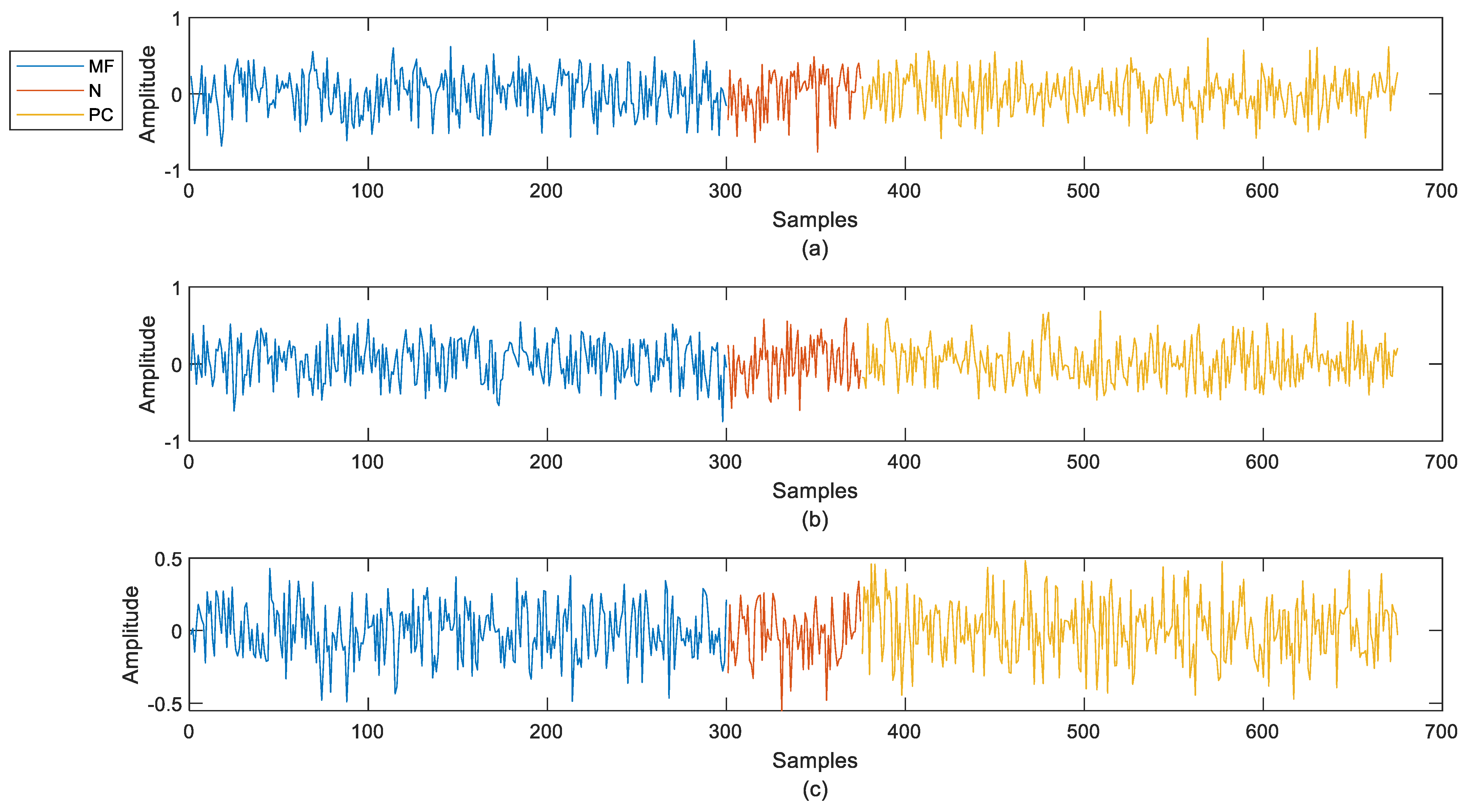
Figure 3a–c showcase the three datasets (A, B, and C, respectively) recorded using the first microphone channel (mic1). These signals highlight a clear recording imbalance, with the normal operating mode receiving fewer samples compared to PC and MF. Additionally, the signals appear highly variable and almost random, underscoring the challenges inherent in dealing with such highly dynamic data and emphasising the need for sophisticated preprocessing. Additionally, comparing datasets A, B, and C reveals a progressive increase in variability, amplitude, and fluctuations over time. This trend indicates that the complexity of the learning problems escalates with each dataset, making subsequent datasets increasingly challenging to analyze and model.

Additionally, to gain more insights into the complexity of raw data signals of datasets A, B, and C, we conducted a preliminary analysis based on three key metrics: variability, amplitude, and fluctuations over time. These metrics were quantified using standard deviation, range, and approximate entropy, denoted in Equations (1)–(5) respectively. Standard deviation $\delta$ measures variability, with $x_i$ representing the signal values, N the number of observations, and $\mu$ the mean of the signal. $\mathsf{\Omega }$ is the amplitude that captures the range of the signal values. Approximate entropy $\eta$ quantifies the fluctuations over time, where $m$ is the embedding dimension, tol is the tolerance (typically set to $0.2 \delta$. The function ${\varphi }^m\left(tol\right)$ is given by (4). Here, $C_i^m\left(tol\right)$ counts the number of m dimensional vector pairs within tol. Finally, complexity quantification CQ is assessed by the sum of the variability, amplitude, and fluctuations over time as in (5).

$$\sigma =\sqrt{{\displaystyle \frac{1}{N}}\sum _{i=1}^N{\left(x_i-\mu \right)}^2}$$

(1)

$$\mathsf{\Omega }=max\left(x\right)-min\left(x\right)$$

(2)

$$\eta \left(m,tol,N\right)={\varphi }^m\left(tol\right)-{\varphi }^{m+1}\left(tol\right)$$

(3)

$${\varphi }^m\left(tol\right)={\displaystyle \frac{1}{N}}-m+1\sum _{i=1}^{N-m+1}ln\left(C_i^m\left(tol\right)\right)$$

(4)

$$CQ=\sigma +\mathsf{\Omega }+\eta$$

(5)

In this work, the complexity quantification $CQ$ was calculated for datasets A, B, and C, resulting in values of 3.2697, 3.5754, and 3.5799, respectively. These findings confirm previous conclusions, demonstrating a progressive increase in complexity from dataset A to dataset C.

2.2. Dataset Preprocessing Methodology

Data preprocessing involves handling three datasets: A, B, and C. Each dataset undergoes a series of steps to extract both inputs and labels from the audio-recorded files. Critical data processing steps are carried out to ensure the quality and relevance of the variables. Firstly, after uploading the files, they are subjected to several processing steps, including scaling, extraction, filtering, denoising, and outlier removal. Scaling ensures that data is normalised, which helps improve the performance and convergence of machine learning models. Extraction helps in providing more meaningful patterns and capturing important information about drone health for each class. Filtering and denoising are applied to remove any unwanted noise and smooth the data, making it cleaner and more accurate for analysis. Outlier removal helps eliminate any anomalous data points that could skew the results.

For the labels, specific ordinal coding is applied to categorise each class. This approach is chosen because ordinal coding preserves the order and ranking of classes, which can be important for certain types of analysis and modelling where the relative importance or ranking of classes matters [33,34]. In this case, ordinal coding helps analyze the model as a sort of regression process and provides an easier way to quantify uncertainty.

After the initial preprocessing steps, data balancing is performed. This is crucial to ensure that the dataset is not biased towards any particular class. Balanced data helps in improving the performance and generalisation of the machine learning models, leading to more reliable and accurate results.

During the feature extraction phase, various statistical and frequency domain features are extracted from the recorded acoustic emission signals, including mean, standard deviation, skewness, kurtosis, peak-to-peak, RMS, crest factor, shape factor, impulse factor, margin factor, and energy [35]. The data is normalised and smoothed to ensure consistency, with median filtering applied to further reduce noise. Wavelet denoising is used to clean the data and handled appropriately to maintain dataset integrity [36]. Outliers are iteratively removed to enhance the quality of the dataset, employing different outlier detection methods such as median analysis, Grubbs’ test, mean analysis, and quartile analysis [37]. These methods are applied for a specified number of iterations to ensure the dataset is free from anomalies that could skew the results. After outlier removal, a smoothing algorithm is used to reduce noise and fluctuations, and the smoothed data is scaled to a range of [0, 1] [38,39]. This normalisation enhances the consistency and performance of subsequent analyses or modelling efforts.

Class imbalances in the dataset can negatively impact the performance of machine learning models. To address this issue, the SMOTE (Synthetic Minority Over-sampling Technique) algorithm is applied [40,41]. SMOTE generates synthetic samples for the minority classes, ensuring equal representation of all classes in the dataset. This balancing act helps improve the model’s performance and reliability.

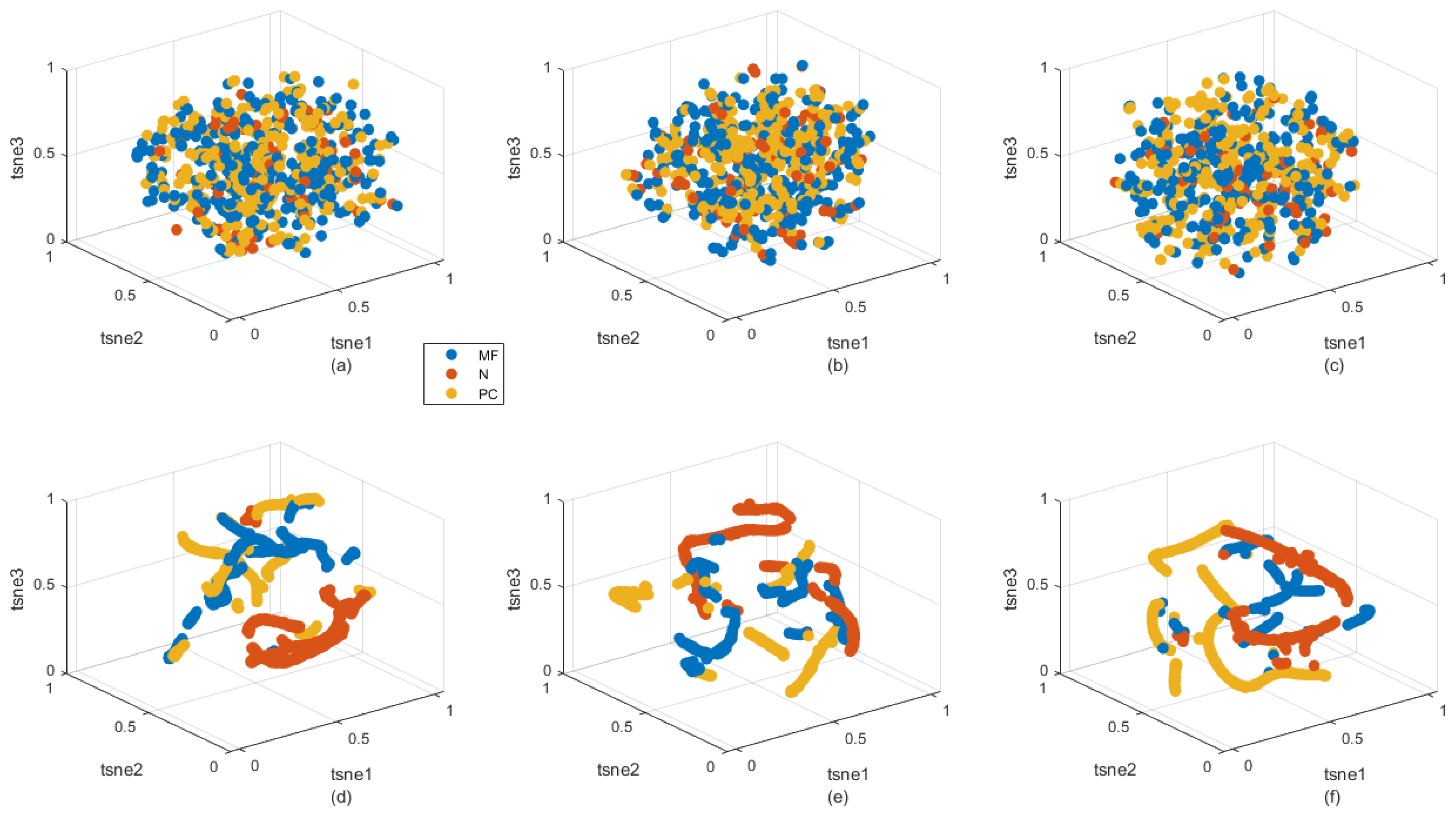
Figure 4 presents both the raw data (Figure 4a–c) and the results after preprocessing (Figure 4d–f). This visualisation uses 3D t-distributed Stochastic Neighbor Embedding (t-SNE) representations to illustrate the distribution of the datasets. In the raw data, the scatter plots demonstrate a high level of overlap and cardinality, making it difficult to distinguish between classes. In contrast, the preprocessed data shows a more separable structure, indicating improved class distinction. Furthermore, similar to Figure 3, a comparison of subfigures of Figure 4d–f reveal an increase in complexity with datasets A, B, and C respectively. This trend signifies that, even in the preprocessed data, the learning problem’s complexity escalates across the datasets.

Accordingly, the comprehensive preprocessing pipeline ensures that the drone acoustic emission data is thoroughly prepared for subsequent analysis or machine learning tasks. This leaves the next complexity reduction step to advanced representation learning algorithms, facilitating more effective and accurate modelling.

3. Methods

This section is dedicated to explaining UBO-MVA-EREX comprehensively, covering both the model architecture and the objective function to be minimised by the Bayesian optimisation algorithm during hyperparameter tuning. Within this context, the objective function subsection will delve into both confidence interval and prediction interval features to provide a detailed understanding.

3.1. MVA-EREX

The MVA-EREX in this work follows the same basic learning rules of the Multiverse Recurrent Expansion with Multiple Repeats (MV-REMR) philosophy [23], with some additional improvements in both learning speed and the representativeness of IMTs. As illustrated in the diagram of Figure 5, the ELM model is trained at each round using inputs $x_k$ at each round $k$. Starting from round 2, $x_k$ will be the same as the collected IMTs. The novel aspect of MVA-EREX is that it introduces new improvements to both feature mapping and estimated targets of IMTs, allowing for both simple and informative feature spaces.

Regarding feature mappings, a series of dimensionality reduction algorithms, including PCA, dropouts, and pruning of neurons, were utilised according to the retained variance ratio $v_{ratio}$, dropout ratio $d_{ratio}$, and pruning ratio $P_{ratio}$, respectively. This process of feature mapping is referred to as ${\rho }_1$.

Concerning the estimated targets $\tilde{y}$ of ELM model at each round $k$, they were subjected to augmented representations via polynomial mapping [42,43], creating a multiverse representation controlled by the hyperparameter $A_{degree}$, which represents the degree of the polynomial function. This specific augmentation process is denoted as ${\rho }_2$. This process is illustrated in Formula (1).

Formula (6) represents the obtained IMTs at each round, where $H_k$ represents the hidden layer of the ELM model obtained via Formula (7). $a_k$ are the randomly generated input weight matrices and $b_k$ are the bias vectors, and $f$ represents an activation function. ${\tilde{y}}_k$ are the estimated targets at each round, which were obtained by mapping the hidden layer to the output layer using the output weight matrices ${\beta }_k$, as in Formula (8). ${\beta }_k$ were obtained from calculating the Moore-Penrose pseudo-inverse of $H_k$ matrices, as indicated in Formula (9). ${H_k}^{\prime }$ is the transpose of $H_k$, $C$ is a regularisation parameter based on the $l_2$ norm optimisation, $I$ is an identity matrix, and $y_k$ were the desired targets.

$$x_{k+1}=[x_k,{\rho }_1\left( H_k\left(x_k\right)\right),{\rho }_2\left( {\tilde{y}}_k\right)]$$

(6)

$$H_k\left(x_k\right)=f(a_k{x}_k+b_k)$$

(7)

$${\tilde{y}}_k={\beta }_k{H}_k\left(x_k\right)$$

(8)

$${\beta }_k=\left(H_k\left(x_k\right)H_k{\left(x_k\right)}^{\prime }\right)+CI\left(y_k\right)$$

(9)

The goal of this architecture is to enable the learning models, starting from the second round, to comprehend both the representations learned from previous models and their behaviours in response to specific learning parameters such as weights, biases, and other hyperparameters. In essence, the subsequent models are designed to integrate the entirety of the previous models’ knowledge, thereby providing the next model with what is believed to be an additional layer of awareness. This approach fundamentally differs from classical deep learning, where models primarily focus on understanding the representations of the data alone. In traditional deep learning, the emphasis is on how the models interpret the data and react to it, without incorporating a deeper understanding of the models’ own previous states and behaviours. The MVA-EREX architecture, by contrast, seeks to enhance learning by ensuring that each successive model iteration is informed not only by the data but also by the comprehensive experiences and adaptations of the prior models, leading to a more robust and informed learning process. Figure 5 also shows the objective function $obj$ related to hyperparameters optimisation based on uncertainty quantification. This aspect will be further explained in the subsequent sections.

3.2. Uncertainty Quantification

For uncertainty quantification, both confidence intervals and prediction intervals are used focusing on their widths to build the objective function [44,45]. Confidence intervals estimate the range within which the true mean lies, reflecting precision and influenced by sample size and variability. Prediction intervals estimate the range for future observations, considering both mean estimation uncertainty and data variability. By incorporating interval widths into the objective function, the model aims to minimise uncertainty, enhancing prediction reliability and accuracy. This dual approach comprehensively assesses uncertainty in both mean values and future observations. This section accordingly introduces and explains this dual approach for uncertainty quantification.

3.2.1. Confidence Interval Features

To calculate confidence intervals $CI$ based on the z-score, the residuals, the differences between actual values $y_k$ and predicted values ${\tilde{y}}_k$, are computed as in (10). Next, the standard deviation of these residuals, denoted as ${\delta }_k$ is determined as in (11). Using the desired confidence level (i.e., 99% in this work), the corresponding z-score can be determined analytically. The margin of error is then calculated by multiplying the z-score with sigma. Finally, the interval width ${CI}_{w\left(k\right)}$ is twice the margin of error as addressed by (12).

$$r_k=y_k-{\tilde{y}}_k$$

(10)

$${\delta }_k={\displaystyle \frac{1}{n}}\sum _{i=1}^n\left(r_k\right(i\left)\right)$$

(11)

$${CI}_{w\left(k\right)}=2z{\delta }_k$$

(12)

3.2.2. Prediction Interval Features

To calculate prediction intervals $PI$, a linear regression model is first fit using the independent variable $x_k$ and the dependent variable $y_k$. The value for new predictions $x_{k\left(new\right)}$ is then used, representing the point at which the prediction is made. Similar to confidence intervals, residuals are computed to determine the standard deviation of the residuals, applicable to both new unseen samples and previous ones as in (13). With the desired confidence level (i.e., 99% in this work), the critical value of the t-distribution $t_{\alpha /2}$ is calculated, considering the degrees of freedom $d_f$, which is the number of observations $n_c$ (samples) minus the number of model coefficients, as shown in (14). The sum of squares of the deviations of $x_k$ from its mean is then computed and used to calculate a term inside the square root of the prediction interval formula, as shown in (15). The margin of error for the prediction interval is derived by multiplying $t_{\alpha /2}$ with the standard deviation and the square root term $S_{term}$. Consequently, the width of the prediction interval is twice the margin of error, providing a measure of uncertainty for predictions at a specified confidence level, as shown in (16). This method ensures a robust and reliable calculation of prediction intervals, accounting for both model and data variability.

$$d_f=n-n_c$$

(13)

$$t_{\alpha /2}=tinv(1-{\displaystyle \frac{1-99\%}{2}}, d_f)$$

(14)

$$S_{term}=2\sqrt{1+{\displaystyle \frac{1}{n}}+{\displaystyle \frac{x_{k\left(new\right)}-\overline{x_k}}{{\sum }_{i=1}^n(x_k-\overline{x_k})}}}$$

(15)

$${PI}_{w\left(k\right)}=2\left(S_{term}{t}_{\alpha /2}\right)$$

(16)

3.2.3. Uncertainty Objective Function

The objective function used in this case to quantify uncertainty incorporates features from both CI and PI. Specifically, the widths of these intervals, ${CI}_{w\left(k\right)}$ and ${PI}_{w\left(k\right)}$ respectively, are the key metrics that need to be optimised. The objective function, as shown in Formula (17), is the sum of these two widths and is designed to be minimised using a Bayesian method for hyperparameter tuning. By minimising this combined interval width, the goal is to achieve a model that is both accurate and reliable in its predictions while effectively managing uncertainty. This combined approach ensures that both the confidence in the model’s predictions and the prediction accuracy are taken into account, leading to a more robust and trustworthy model.

$$obj={CI}_{w\left(k\right)}+{PI}_{w\left(k\right)}$$

(17)

4. Results

This section presents and discusses the results obtained in this work. For clarity, the results are organised to first showcase the performance of the UBO-MVA-EREX methodology, our main proposed approach. Detailed illustrations and analyses of UBO-MVA-EREX’s performance metrics are provided, highlighting its effectiveness and strengths. Subsequently, a comparative analysis is conducted, where UBO-MVA-EREX is benchmarked against other existing methodologies. This structured presentation allows for a comprehensive understanding of UBO-MVA-EREX’s capabilities and its relative performance in the context of similar approaches, providing insights into its practical advantages and potential areas for further improvement.

The illustration of results will follow a structured methodology, starting with visual metrics such as convergence curves, CIs, PIs, and confusion matrices. These visualisations will be followed by a numerical evaluation and analysis based on tables of error metrics and classification metrics. This approach ensures a thorough examination of UBO-MVA-EREX’s performance from multiple perspectives, both qualitative and quantitative.

To study the UBO-MVA-EREX algorithm, its convergence behaviour was first investigated. The proof provided from this demonstrated that learning from both multiple models’ behaviours (i.e., IMTs) and representations enhances the learning process, enabling the algorithm to acquire additional knowledge with each round $k$. To illustrate this, the coefficient of determination $R^2$ and its variations during the learning process were examined across the three datasets A, B, and C.

Figure 6 illustrates these findings. In Figure 6a–c, the convergence towards better performance is evident for both the training and testing phases. In Figure 6a, corresponding to dataset A, the testing curves almost mirror the training curves, indicating excellent performance. Similarly, Figure 6b shows good convergence with a slight but acceptable gap between the training and testing curves. However, in Figure 6c, related to dataset C, there is a slight deviation in the testing performance, highlighting the increased complexity of dataset C.

An important note in this case is that as complexity increases from datasets A to C, the training process achieves a higher coefficient of determination. This improvement during training may be related to several factors, including the model’s ability to capture more intricate patterns within more complex data. However, this also indicates a tendency towards overfitting, where the model learns the training data too well, including its noise and outliers. On the other hand, the testing performance decreases from dataset A to dataset C, which provides a clear indication of the increasing complexity. This decline in testing performance suggests that while the model fits the training data better, it struggles to generalise to new, unseen data, highlighting the challenges posed by the higher complexity of the datasets. This underscores the trade-off between fitting complex patterns in the training data and maintaining generalisation capabilities on test data, a common issue when dealing with high-complexity datasets.

Overall, these observations in Figure 6 underscore the robustness of the designed algorithm and its ability to maintain fidelity across different datasets. The progressive increase in complexity from dataset A to C, as previously noted in the Materials section during data visualisation, is also clearly reflected in these results. This structured examination helps validate the effectiveness of UBO-MVA-EREX in handling varied and complex datasets.

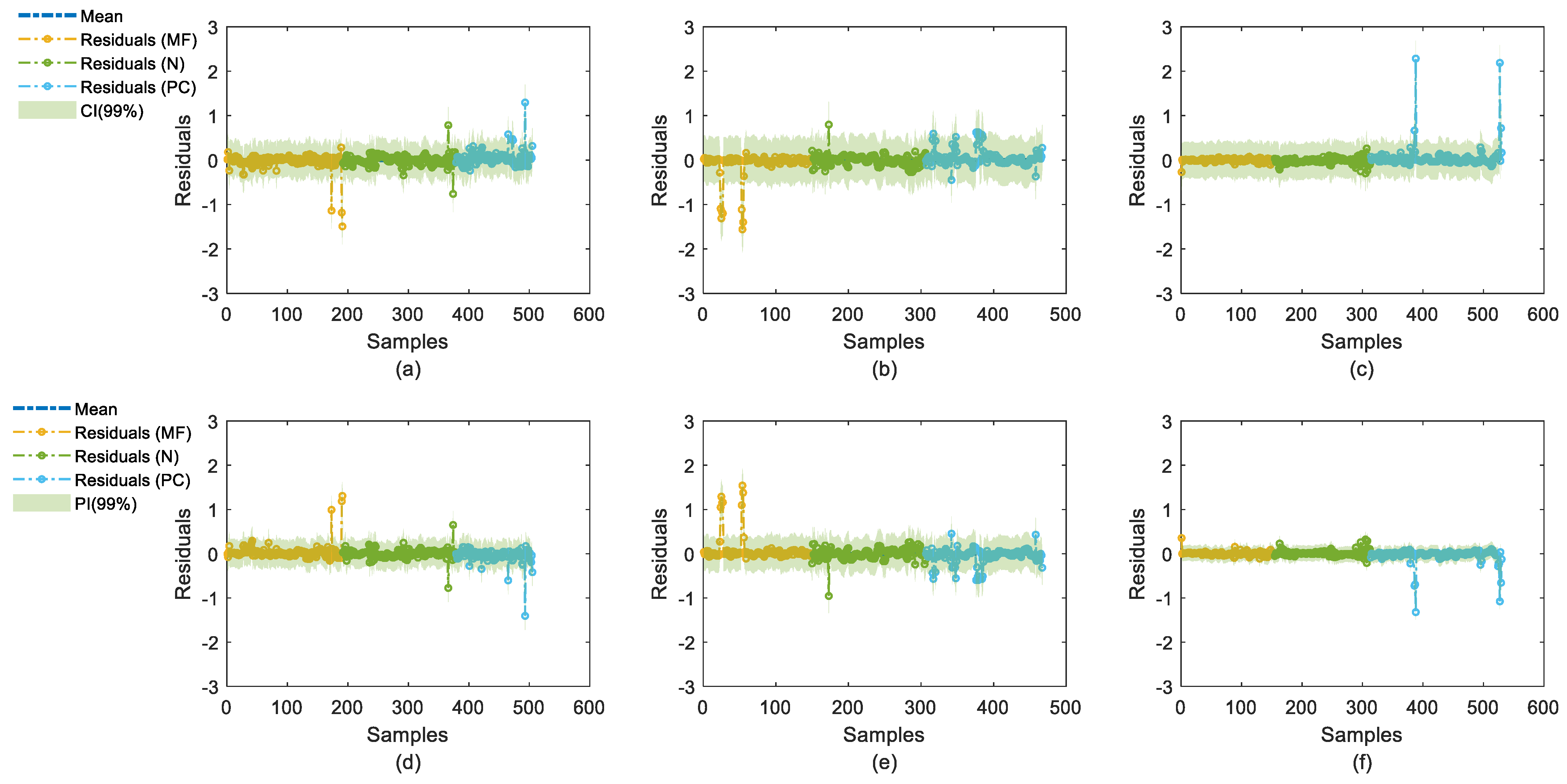
To illustrate uncertainty, Figure 7 presents the residuals from approximating the ordinal codes of the multiclass datasets and their corresponding CIs and PIs. Figure 7a–c show CIs for datasets A, B, and C, respectively, highlighting fluctuations in uncertainty measurements, with an increasing number of fluctuations across datasets A, B, and C. The interval width exhibits a degree of consistency, though it increases somewhat across datasets. Notably, the residuals for the injected faults, PC and MF, display significantly more fluctuations compared to the normal operating condition (N). This indicates that the uncertain measurements, despite the additive noise, are predominantly due to motor malfunctions rather than environmental conditions.

Similar observations can be made from Figure 7d–f for the PIs corresponding to datasets A, B, and C, where the prediction intervals also reflect these trends in interval widths and uncertainty measurements.

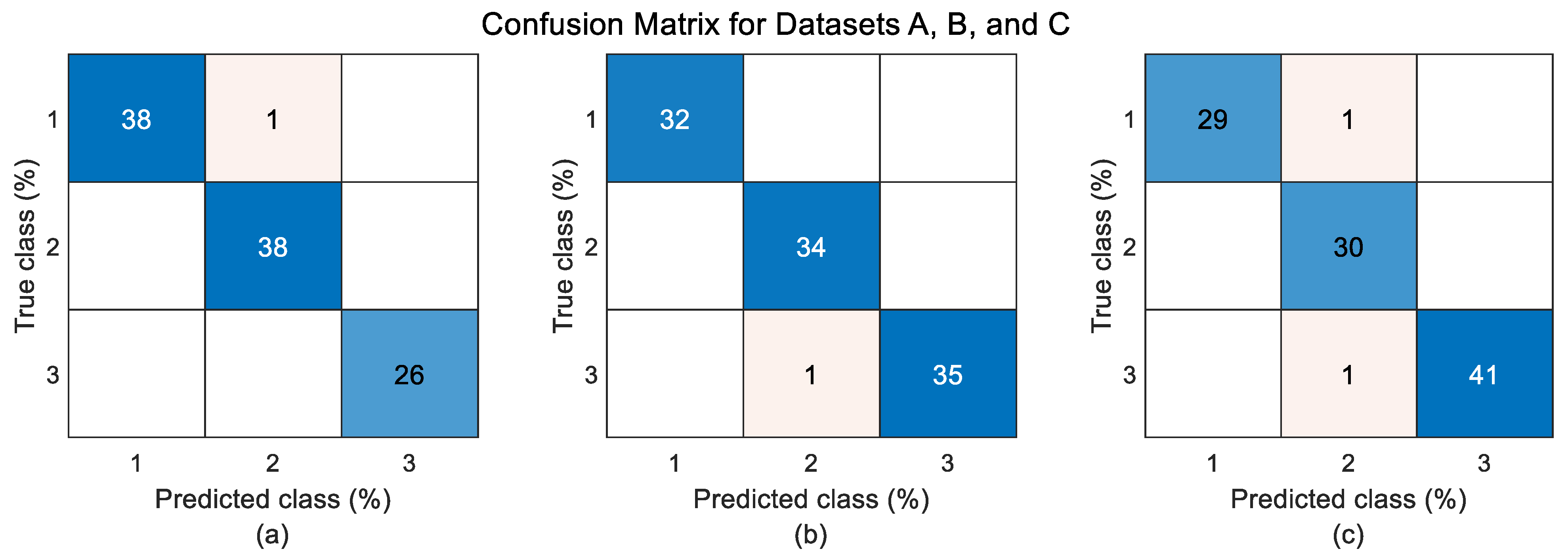
Additionally, the confusion matrices in Figure 8a–c, which illustrate the prediction rates for each class in percentage terms, further confirm the accuracy of the model’s predictions. These matrices provide a clear visualisation of how well the model distinguishes between different classes, highlighting its effectiveness. Moreover, the confusion matrices reveal the increasing complexity and challenges associated with each dataset. Specifically, the accuracy decreases and the misclassification rates increase progressively from dataset A to B, and from B to C. This trend underscores the escalating difficulty in accurately predicting classes as the dataset complexity increases, demonstrating the robustness of the UBO-MVA-EREX methodology in handling varied and dynamic data scenarios.

Table 1. Error metrics results for UBO-MVA-EREX.

	Metric	A	B	C
Training	RMSE	0.14015	0.1515	0.0736
	MAE	0.08189	0.0765	0.0430
	MSE	0.01964	0.0229	0.0054
	R2	0.96836	0.9646	0.9920
Testing	RMSE	0.15745	0.1997	0.1561
	MAE	0.08253	0.0923	0.0531
	MSE	0.02479	0.0399	0.0243
	R2	0.95959	0.9398	0.9644

presents the error metrics results for UBO-MVA-EREX methodology across three datasets: A, B, and C. The metrics are divided into training and testing phases, showcasing Root Mean Square Error (RMSE), Mean Absolute Error (MAE), Mean Squared Error (MSE), and the coefficient of determination (R²). Additionally, the table includes the objective search time during training. In the training phase, dataset C exhibits the lowest RMSE (0.0737), MAE (0.0431), and MSE (0.0054), and the highest R² (0.9921), indicating superior performance. Dataset A follows with RMSE, MAE, and MSE values of 0.1402, 0.0819, and 0.0196 respectively, and an R² of 0.9684. Dataset B shows slightly higher errors with an RMSE of 0.1515, an MAE of 0.0766, an MSE of 0.0230, and an R² of 0.9647. During Testing, the errors increase slightly, with dataset A having an RMSE of 0.1575, MAE of 0.0825, MSE of 0.0248, and R² of 0.9596. Dataset B records higher errors with an RMSE of 0.1998, MAE of 0.0923, MSE of 0.0399, and R² of 0.9398. Dataset C maintains lower errors in comparison with an RMSE of 0.1562, MAE of 0.0531, MSE of 0.0244, and R² of 0.9644. These results highlight the effectiveness of the UBO-MVA-EREX methodology in handling varying complexities across datasets, demonstrating particularly strong performance on the most complex dataset, C.

Table 2. Classification metrics results for UBO-MVA-EREX and LSTM.

Method	UBO-MVA-EREX			LSTM
Dataset	A	B	C	A	B	C
Accuracy	0.9980	0.9957	0.9943	0.9168	0.9100	0.9207
Precision	0.9982	0.9958	0.9938	0.9260	0.9284	0.9218
Recall	0.9980	0.9957	0.9947	0.9205	0.9096	0.9282
F1-Score	0.9981	0.9958	0.9942	0.9233	0.9189	0.9250
Objective Search Time (s)	0.12350	0.0616	0.0885	3.3178	1.2141	10.2541

presents the classification metrics results for both the UBO-MVA-EREX methodology and LSTM for comparative analysis. The metrics include accuracy, precision, recall, and F1 scores, which are essential for evaluating the performance of classification models. First, the UBO-MVA-EREX model achieves high accuracy across all datasets, with values of 0.9980 for dataset A, 0.9957 for dataset B, and 0.9943 for dataset C. The precision values are similarly high, at 0.9982 for dataset A, 0.9959 for dataset B, and 0.9938 for dataset C, reflecting its capability to minimise false positives. The recall values are 0.9981 for dataset A, 0.9957 for dataset B, and 0.9948 for dataset C, demonstrating the model’s ability to identify most of the actual positive cases. The F1-Scores, which balance precision and recall, are 0.9981 for dataset A, 0.9958 for dataset B, and 0.9943 for dataset C, indicating the overall robustness and reliability of the UBO-MVA-EREX model in classification tasks. The objective search time, which reflects the duration for optimising the model’s hyperparameters using Bayesian optimisation, is 0.1235 for dataset A, 0.0617 for dataset B, and 0.0886 for dataset C. These metrics collectively highlight the model’s strong performance in accurately classifying data, with particularly high precision and recall, ensuring both the correctness and completeness of its predictions. The slight decrease in performance from dataset A to dataset C reflects the increasing complexity and challenges posed by the datasets, yet the UBO-MVA-EREX methodology maintains high effectiveness across all scenarios. Second, LSTM [46] model’s hyperparameters are also optimised via Bayesian algorithms, but, with the objective function being the RMSE. For dataset A, the LSTM model achieves an accuracy of 0.9168, a precision of 0.9261, a recall of 0.9206, and an F1 score of 0.9233. Dataset B shows an accuracy of 0.9101, a precision of 0.9285, a recall of 0.9096, and an F1 score of 0.9190. Dataset C has an accuracy of 0.9208, a precision of 0.9218, a recall of 0.9282, and an F1 score of 0.9250. Computational time showcases a massive decrease compared to UBO-MVA-EREX. Comparing these results with those of UBO-MVA-EREX, UBO-MVA-EREX consistently outperforms LSTM in all metrics and datasets with less computational costs. UBO-MVA-EREX’s higher accuracy, precision, recall, and F1 score demonstrate its superior capability in handling complex and dynamic data, making it a more effective model for classification tasks than the LSTM model. Given the extensive range of metrics utilised and the comprehensive dataset comparisons, the comparison with LSTM is sufficient to underscore the effectiveness of the UBO-MVA-EREX methodology.

Table 3. Best obtained hyperparameters via Bayesian optimisation of uncertainty objective function.

Dataset	Neurons	Activation	Regularisation	Rounds	${\mathit{v}}_{\mathit{r}\mathit{a}\mathit{t}\mathit{i}\mathit{o}}$	$d_{ratio}$	$P_{ratio}$	$A_{degree}$
A	100	sigmoid	0.0190	14	22	73	75	2
B	99	sigmoid	0.0408	5	24	47	82	2
C	99	sigmoid	0.0319	7	36	37	66	2

provides the hyperparameters optimised by the UBO-MVA-EREX methodology These settings include the number of neurons, the activation function, the regularisation parameter, the number of rounds, the retained variance ratio $v_{ratio}$, the dropout ratio $d_{ratio}$, the pruning ratio $P_{ratio}$, and the polynomial degree $A_{degree}$. For dataset A, the model utilises 100 neurons with a sigmoid activation function. The regularisation parameter is set at 0.0190. The training process spans 14 rounds, with a retained variance ratio of 22%, a dropout ratio of 73%, a pruning ratio of 75%, and a polynomial degree of 2. For dataset B, the model uses 99 neurons, also with a sigmoid activation function. The regularisation parameter is 0.0408. The training comprises 5 rounds, a retained variance ratio of 24%, a dropout ratio of 47%, a pruning ratio of 82%, and a polynomial degree of 2. For dataset C, the model again uses 99 neurons with a sigmoid activation function. The regularisation parameter is 0.0319. There are 7 rounds of training, with a retained variance ratio of 36%, a dropout ratio of 37%, a pruning ratio of 66%, and a polynomial degree of 2. These configurations illustrate the flexibility and adaptability of the UBO-MVA-EREX methodology in handling varying complexities across different datasets. The adjustments in hyperparameters such as the number of neurons, regularisation, and ratios of retained variance, dropout, and pruning, reflect the need to balance model complexity, overfitting, and computational efficiency.

5. Conclusions

This study introduces the UBO-MVA-EREX methodology, a novel approach designed to enhance fault diagnosis in drones by integrating multiple model behaviours and representations while accounting for acoustic emission measurement uncertainty. Through a methodologically sound pipeline of data preprocessing applied to highly variable data from three acoustic emission datasets with multiclass classification challenges, the findings consistently demonstrate the superiority of UBO-MVA-EREX over traditional methods such as LSTM. This superiority is evident across diverse datasets, highlighting the robustness and efficacy of the methodology. Detailed analyses reveal significant improvements in various metrics, including error rates, classification accuracy, uncertainty quantification, and computational efficiency. These enhancements are illustrated through both visual representations (e.g., curves and figures) and numerical values, particularly as dataset complexity increases, whether transitioning from one operating condition to another or between different datasets. The methodology’s effectiveness in managing dynamic data characterised by high variability and complexity underscores its potential for broader applications. Moreover, the comprehensive preprocessing pipeline, which includes feature extraction, denoising, outlier management, and class balancing, significantly contributes to the model’s success. In summary, UBO-MVA-EREX marks a significant advancement in machine learning, providing a powerful tool for precise and reliable classification tasks in complex fault diagnosis scenarios. Future work will focus on enhancing this approach by considering data preprocessing, tuning hyperparameters, improving uncertainty quantification, and exploring its applicability to other domains. Additionally, it is important to consider more data malfunctions and characteristics such as concept drift and multivariate conditions. Ongoing algorithmic improvements will aim to continually improve the efficiency and performance of the methodology.