Performance Prediction of the Elastic Support Structure of a Wind Turbine Based on Multi-Task Learning

Abstract

The effectiveness of a wind turbine elastic support in reducing vibrations significantly impacts the unit’s lifespan. During the structural design process, it is necessary to consider the influence of structural design parameters on multiple performance indicators. While neural networks can fit the relationships between design parameters on multiple performance indicators, traditional modeling methods often isolate multiple tasks, hindering the learning on correlations between tasks and reducing efficiency. Moreover, acquiring training data through physical experiments is expensive and yields limited data, insufficient for effective model training. To address these challenges, this research introduces a data generation method using a digital twin model, simulating physical conditions to generate data at a lower cost. Building on this, a Multi-gate Mixture-of-Experts multi-task prediction model with Long Short-Term Memory (MMoE-LSTM) module is developed. LSTM enhances the model’s ability to extract nonlinear features from data, improving learning. Additionally, a dynamic weighting strategy, based on coefficient of variation weighting and ridge regression, is employed to automate loss weight adjustments and address imbalances in multi-task learning. The proposed model, validated on datasets created using the digital twin model, achieved over 95% predictive accuracy for multiple tasks, demonstrating that this method is effective.

1. Introduction

Large wind turbines can experience vibrations due to their own operations as well as external factors, which can have adverse effects on the entire turbine system. To ensure stable and reliable wind turbines operations over extended periods, it is crucial to install vibration dampers at critical locations within the wind turbine system [1]. The elastic support of a wind turbine plays a vital role in reducing vibrations, and its structural mechanical performance indicators, such as stiffness and stress under rated conditions, directly influence the effectiveness of vibration reduction and the lifespan of the elastic support. Therefore, during the design process of a wind turbine elastic support, careful attention must be paid to multiple structural performance indicators.

During the structural design process, designers must consider various performance indicators (PIs) of the structure, and establishing the relationship between these PIs and design parameters has been a longstanding topic of discussion among engineers. Mathematical models can be constructed based on experimental design and analysis of multiple experimental results to describe the relationship between PIs and design variables [2]. However, conducting multiple physical experiments to obtain data can be expensive.

With advances in computer science and hardware capabilities, it has become feasible to obtain simulation data that align with actual experimental conditions through simulation experiments [3]. Simulation experiments have gained widespread recognition and have become an essential tool in assisting product structure design [4]. Many scholars are currently investigating the relationship between design parameters and PIs through simulation experiments. For instance, Xiao et al. [5] utilized orthogonal experimental design and finite element simulation to identify the main factors influencing the static stiffness of rubber dampers and designed an optimization scheme for rubber dampers based on sensitivity analysis. Moreover, Dong et al. [6] established a finite element model of tibia implants and combined finite element analysis with the Taguchi orthogonal experiment method to analyze the influence of multiple design variables on the peak contact pressure of the implant, providing guidance for the accurate implantation of tibial implants. While mathematical models based on experimental design can describe the relationships between multiple factors, traditional models may struggle to accurately capture complex nonlinear relationships. This requires the use of more advanced modeling methods.

In recent years, with the rapid advancement of artificial intelligence (AI) technology, machine learning techniques have found widespread application in the engineering field, with neural networks emerging as a popular choice for engineering design. Neural networks exhibit superior capabilities compared to traditional modeling methods in handling complex data and extracting nonlinear relationships [7]. Numerous scholars have applied machine learning to the field of vibration damper design. For instance, Li et al. [8] investigated the relationship between rubber bushes and various design parameters using artificial neural networks (ANNs). They calculated the radial stiffness of rubber bushes under different cross-sectional shapes and axial pre-compression conditions through simulation. Similarly, Dai et al. [9] examined the dynamic performance of rubber bushes under different frequencies, amplitudes, and temperature excitations, and they developed a hybrid neural network model trained on performance data to accurately represent the dynamic performance of rubber bushes under diverse conditions. In addition, Dai et al. [10] integrated a physical parameter model with a neural network model, considering structural parameters of the damper in the former and describing hydraulic damper characteristics in the latter. The hybrid model, validated through physical experiments, effectively simulated the dynamic performance of hydraulic dampers under various operating conditions. Furthermore, Zheng et al. [11] proposed a method of combining ANN with mechanical modeling to experimentally measure static and dynamic characteristics of rubber mounts, hydraulic mounts, and shock absorbers. They deployed experimental data for neural network training, realizing the prediction of nonlinear dynamic characteristics of automotive mounts and shock absorbers. These studies demonstrate a growing number of research studies on the application of machine learning in engineering, with significant outcomes in enhancing design processes and optimizing engineering solutions.

Compared to prediction models using neural network technology, traditional prediction models still have many applications in engineering design. Rıdvan et al. [12] used orthogonal experimental analysis to study the effects of nozzle collection parameters and fluid composition parameters on the performance of electro-spray cooling, and they constructed a prediction model using the response surface methodology to optimize the electro-spray nozzle. Li et al. [13] employed the optimal hypercube experimental design to examine the relationship between wind turbine airfoil design parameters and performance, and used multiple regression models to predict the impact of various design parameters on performance, analyzing the highly nonlinear relationships between design parameters and performance. Cheng et al. [14] developed a mobile pump truck model and used finite element simulation to analyze the impact of design variables in the truck frame on overall pump truck performance, constructing a response surface prediction model based on simulation data to achieve the lightweight design of the pump truck frame. Non-neural-network-based prediction models require less data, but if the data exhibit complex nonlinear relationships, the models’ predictive accuracies are poor. Compared to traditional prediction models, prediction models based on neural network technology can effectively extract complex features from data and learn patterns. Hasan et al. [15] used CFD analysis to study the effects of refrigerator design parameters on performance, and they used artificial neural network technology to fit the relationship between design parameters and refrigerator performance, optimizing the refrigerator’s performance and reducing the annual energy consumption. Lahcen et al. [16] analyzed the impact of 3D printing process parameters on the ultimate tensile strength of printed parts through extensive experiments and constructed a prediction model using artificial neural network technology to optimize the process parameters. The results showed that compared to linear regression prediction models, neural network prediction models can more accurately optimize process parameters. Compared to traditional prediction models, neural network prediction models can better fit complex relationships between data and achieve more accurate predictions, but they require larger datasets to train the model and ensure predictive accuracy [17]. In engineering, physical experiments are expensive, and simulations involving complex scenarios, such as nonlinear structures, complex materials, and multi-physical field coupling, often require significant computational resources. Consequently, network models are frequently trained with small sample datasets. During the design process, various factors must be considered. If traditional neural network models, such as back-propagation (BP) [18], radial basis function (RBF) [19], and multi-layer perceptron (MLP) [20] are employed to capture the relationships between design parameters and multiple PIs, then multiple neural network models must be trained, each responsible for learning a single PI task. This approach increases the workload and time costs, associated with training and maintaining multiple independent neural network models. Furthermore, the absence of interaction between models can result in information silos, where each model learns features and patterns exclusively related to its task and fails to fully exploit correlations between different tasks [21].

In the domain of rubber damper research, most data used to train neural network models are derived from costly physical experiments, resulting in limited data quantities, which affect the training effectiveness of the network models. Additionally, only a few scholars have adopted multi-task learning mechanisms in their neural network models for research purposes. In addressing the challenge of insufficient data due to cost constraints and other factors, some scholars have turned to generative models, such as the variational autoencoder (VAE) [22] and generative adversarial network (GAN) [23], to augment existing datasets. However, these models are predominantly applied in image and text domains, with limited research on their application to time-series and structured data. Additionally, generative models have specific requirements regarding the quantity and quality of the basic dataset, considering the cost of physical experiments and potential errors. Hence, they may not be suitable for this application.

To mitigate experimental costs, some scholars have leveraged digital twin models to generate data for training neural network models. For example, Mao et al. [24] investigated the influence of the non-dimensional plate length and damping value on the berthing damping rate of underwater platforms. They employed computational fluid dynamics (CFD) to calculate berthing damping rate values for various plate lengths and damping values. The simulation results were used to train the BP neural network combined with genetic algorithms (GAs) to generate the optimal design. Moreover, Wang et al. [25] used a BP neural network to model the relationship between weight, dynamic characteristics, and surface shape errors of a large space-based mirror, and its structural parameters, with training data obtained through finite element simulation analysis. Furthermore, Silva et al. [26] employed a finite element simulation model to assess the stress impact of the pedicle screw installation position and direction on the installation area, training a neural network with simulation experimental data to minimize the mechanical stress between the pedicle screw and vertebrae.

Utilizing digital twin models for data generation offers potential cost savings and increases the data available for training network models. However, challenges such as significant deviations between simulation and physical experiment results, as well as a lower data quality, need to be addressed to ensure the effectiveness of network training.

Compared to traditional neural networks, neural network models for multi-task learning typically comprise multiple neural networks within a single framework, such as the Multi-gate Mixture-of-Experts model (MMoE) [27], Progressive Layered Extraction (PLE) [28], and Cross-Stitch Networks (CSNs) [29]. In applied research, Gao et al. [30] developed a multi-task network, named CrackFormer, to identify the starting position, repair scenarios, and morphological features of fatigue cracks. Their study demonstrated improved accuracy and robustness compared to isolated tasks by leveraging knowledge complementarity between tasks. Similarly, Wang et al. [31] utilized MMoE to learn the diagnosis and localization of partial discharges in gas-insulated switchgear. Their research uncovered differences and coupling relationships between diagnosis and localization tasks, achieving superior results compared to single-task networks.

Multi-task learning frameworks can extract features from data through multiple neural networks, facilitate information sharing between tasks, and learn correlations between tasks. This enables effective learning, thereby improving the model’s predictive accuracy and generalization capability [32]. However, multi-task learning often necessitates a larger quantity and higher quality of data to achieve satisfactory training results. Additionally, it may encounter challenges such as overfitting and imbalanced loss decrease between tasks, especially in scenarios with small sample sizes and poor task correlation [33]. Therefore, it is often essential to refine the multi-task learning network framework and the loss function utilized in the model training process when dealing with different types of datasets [34].

To overcome challenges in dataset generation and multi-task learning, this paper presents a novel data generation approach based on the digital twin model. By constructing a digital twin model of the wind turbine elastic support and validating the simulation’s reliability through physical experiments, the study is able to employ the Latin hypercube sampling method for its experimental design to generate simulation data for subsequent training, thus saving time and cost.

To tackle issues related to small sample sizes and nonlinear characteristics in rubber elastic support structure performance data, an enhanced model framework, called MMoE-LSTM, based on the MMoE model, is introduced. The Long Short-Term Memory (LSTM) module is incorporated to enhance the model’s ability to capture the nonlinear complex features of the data, thereby improving the predictive accuracy of the multi-task model.

In addition, to tackle challenges stemming from poor task correlation and limited data availability for learning, this paper proposes employing coefficient of variation weighting to dynamically adjust the weights of each task’s loss in the total loss function [35]. Furthermore, L2 regularization is introduced into the total loss function to prevent the model from excessively relying on a few features, thereby improving the model’s generalization ability on new data and mitigating the risk of overfitting [36].

To sum up, the proposed method is validated using a dataset generated based on the digital twin model. The experimental results highlight the outperformance of the proposed method compared to traditional methods under limited sample conditions. Therefore, the main contributions of this research are summarized as follows:

• An effective data generation method, based on the digital twin model, is proposed to deliver high-quality wind turbine elastic support structure performance datasets suitable for neural network training, yielding a cost saving;
• An improved network model, MMoE-LSTM, is developed based on the MMoE model framework. The LSTM is applied to enhance the model’s ability to capture nonlinear features in the data, enhancing the predictive capabilities of the multi-task model;
• A novel approach, combining coefficient of variation weighting and L2 regularization, is proposed to optimize the total loss function of the multi-task learning. This method tackles challenges and limitations such as overfitting, premature convergence of individual task loss functions, and imbalanced loss reduction between tasks.

Overall, this study proposes a novel approach for generating datasets and training multi-task learning models, particularly in the context of wind turbine elastic support design. Moreover, it provides a valuable resource for engineers and researchers in the field.

2. Methodology

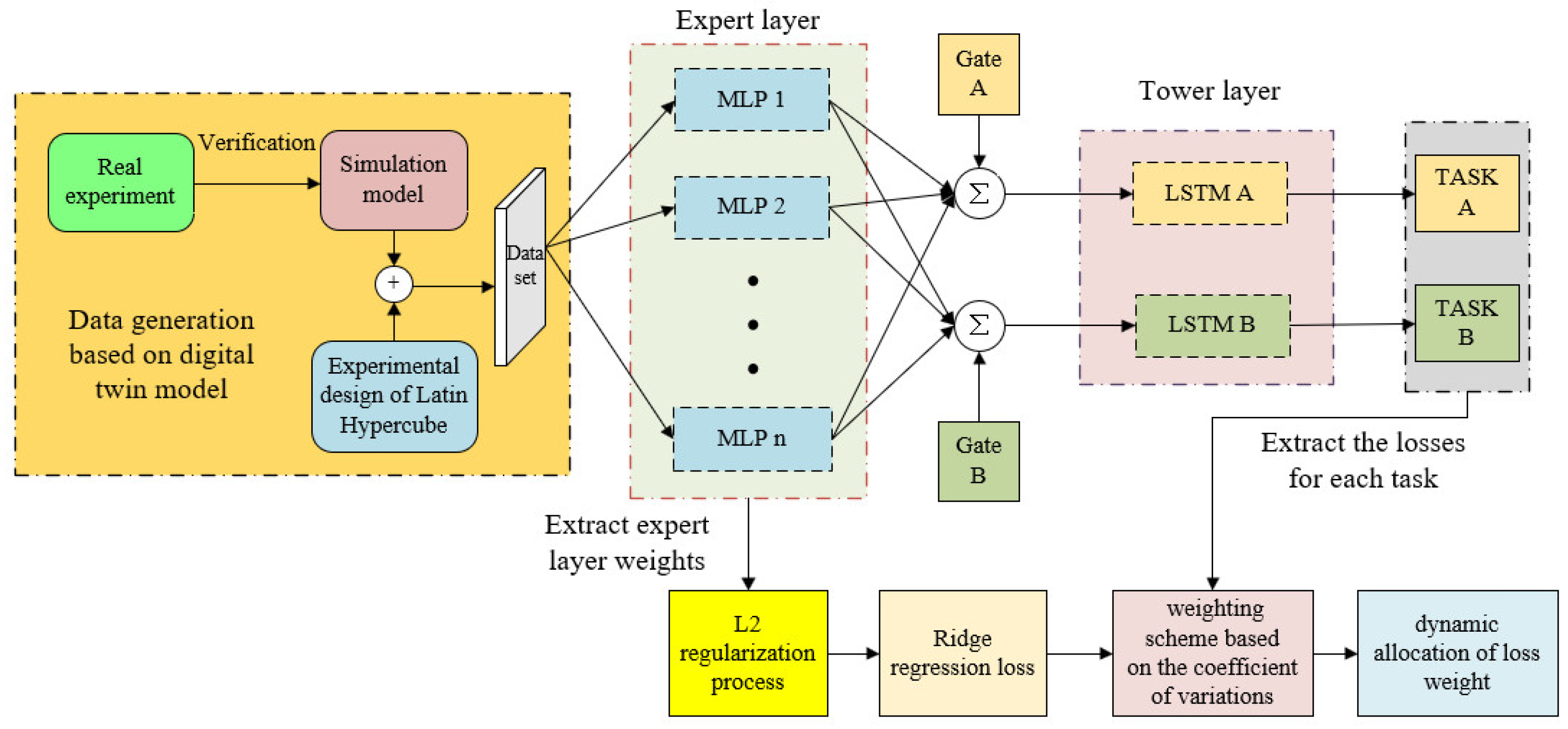
Initially, in this section, a data generation method, based on the digital twin model, is introduced. Consequently, the MMoE-LSTM network structure is presented, consisting of an improvement of the MMoE multi-task network architecture. Finally, the enhanced multi-task loss function, based on coefficient of variation weighting and L2 regularization, is highlighted. The overall workflow is shown in Figure 1.

2.1. Data Generation Based on Digital Twin Model

In the industrial domain, data collection using machine learning techniques is usually a time-consuming and labor-intensive process. Physical experiments can be expensive, while simulation experiments, based on digital twin models, represent a more economical and efficient alternative [37]. However, simulation experiments’ results may deviate from the actual outcomes. Moreover, excessive deviations can seriously affect the quality of the dataset and the training results of the network model. To ensure the simulation quality while balancing the relationship between cost and quality, as depicted in Figure 2, a data generation method, based on the digital twin model, is proposed.

Manufacturing wind turbine elastic supports relies on molds. To conduct physical experiments and test the structural mechanical performance indicators of elastic supports under various structural design parameters, new molds must be manufactured. This involves producing samples for physical testing. Using artificial neural network (ANN) technology to construct performance prediction models requires a substantial amount of experimental data. While physical experiments can yield precise data, the high costs associated with sample manufacturing and experimentation make it impractical to conduct extensive physical tests to provide training data. Digital twin technology, which creates virtual models of physical objects in a digital format and simulates their state in real-world environments, enables digital models to accurately reflect the actual state and behavior of physical entities. This can help researchers reduce experimental costs and conduct a large number of simulation studies, providing data for training ANNs.

Using existing physical test data to validate the reliability of the data generated by the digital twin model, the combination of digital twin technology and artificial neural network (ANN) technology uses data from digital twin models to train ANN-based prediction models. This enables the prediction of various structural performance data of wind turbine elastic supports, avoiding more simulations and computational costs. This study combines digital twin technology with artificial neural network (ANN) technology, leveraging the capabilities of digital twin simulation and the powerful data processing capabilities of ANNs, achieving accurate prediction of the complex structural performance at a lower experimental cost.

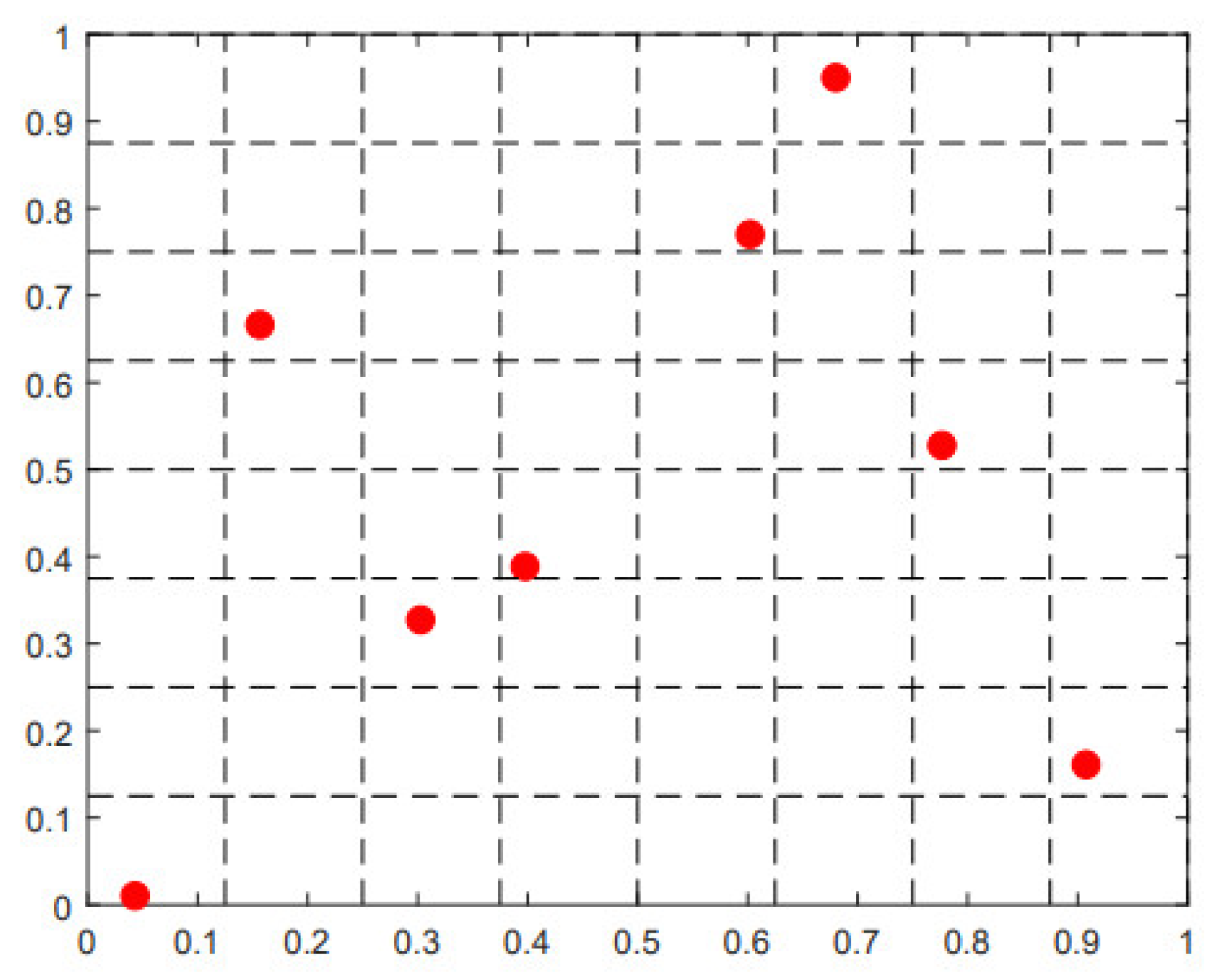
Latin hypercube sampling is a method utilized for selecting sample points within a multi-dimensional space. The primary objective is to generate a set of points that are uniformly distributed across the parameter space [38]. Assuming there are n input variables and m experimental design points, each variable is divided into m levels from the lower to the upper limit values. The value of each variable is randomly chosen from one of the levels, and each variable’s level of values is unique, thus constituting an experimental design point. In a matrix with dimensions m × n, each column represents a variable and each row represents a level. The sampling method is shown in Figure 3, the red dots on each column represent the level represented by a single sample on each parameter dimension.

By adopting Latin hypercube sampling to collect data, a good coverage of the entire parameter range is achieved compared to random sampling. This helps the neural network to learn, more comprehensively, various changes in input features. Therefore, it is an effective way to learn the relationship between input and output features, which enhances the predictive accuracy and generalization ability of the network model.

2.2. Network Model Framework

As already detailed, this study adopted the MMoE-LSTM network model, which is an improvement on the MMoE network model. The MMoE-LSTM network framework includes sub-networks, such as MLP and LSTM.

2.2.1. Multi-Task Learning Network Model

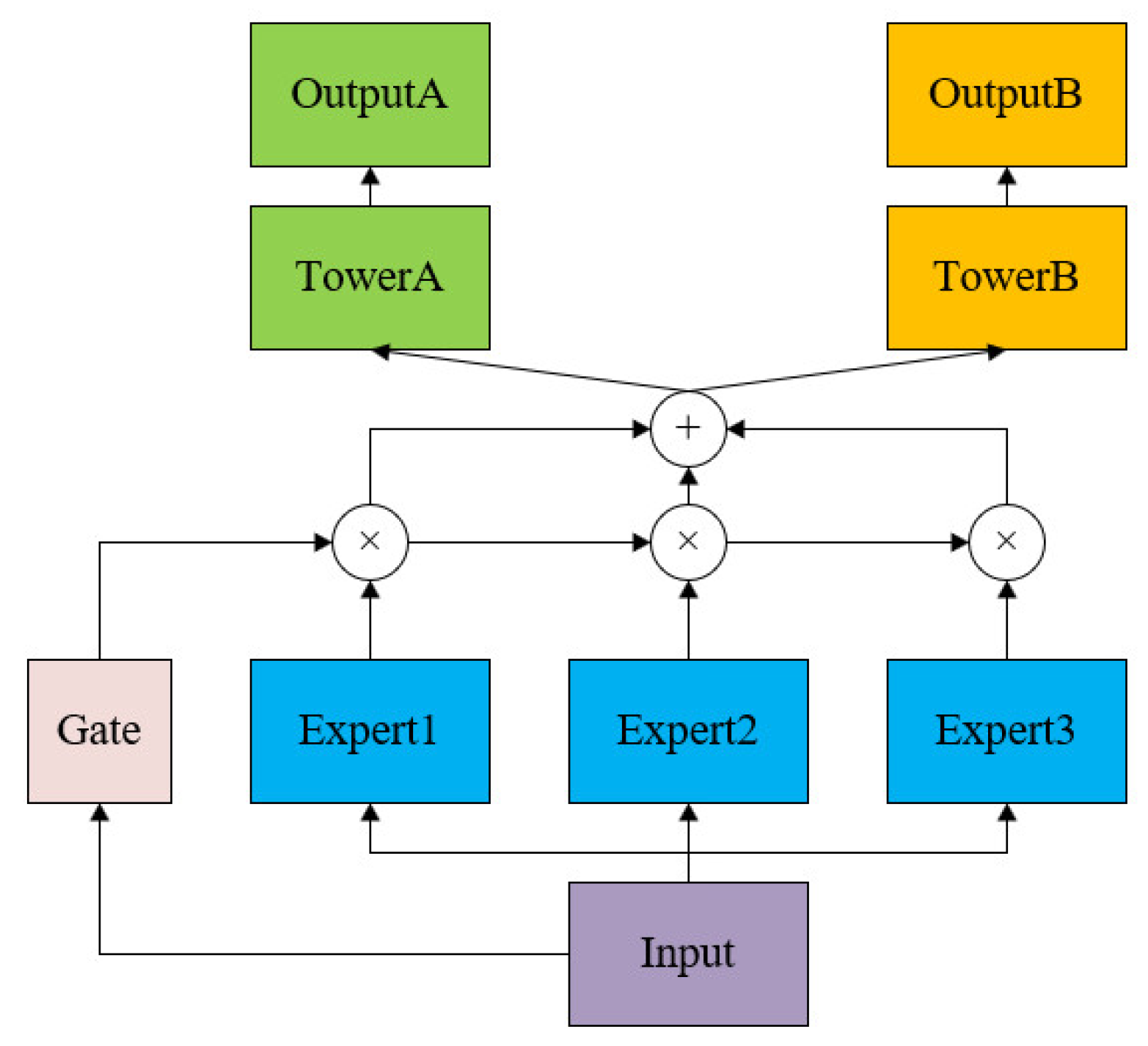
The MMoE model, an improvement of the MoE model, falls under the soft parameter sharing category. The structural framework diagram of the MoE network model, as shown in Figure 4, comprise three main components: an Expert layer, a gating network, and an output layer. The Expert neural network consists of a single-hidden-layer fully connected neural network, and its hidden layer activation function uses a Rectified Linear Unit (ReLU) to enhance the nonlinear mapping and mitigate overfitting. As for the gating network, this dynamically determines the importance of each Expert neural network for different tasks based on the input data. For each input data point, the gating network assigns weights to the output results of each Expert neural network, thereby evaluating the contribution of each Expert neural network to each task. Finally, for the output layer, each task’s output result is processed by a separate Tower neural network. This neural network combines the output results of each Expert neural network with the weights assigned by the gating network to produce the final output of the task results.

The original Mixture-of-Experts (MoE) Model can be formulated as follows [39]:

$$y={\sum }_{i=1}^n{g\left(x\right)}_i{f}_i\left(x\right)$$

(1)

where $\sum _{i=1}^n{g\left(x\right)}_i=1$ and ${g\left(x\right)}_i$, representing the i-th logit of the output of g(x), indicates the probability for expert $f_i$, where $f_i,i=\mathrm{1,2},\dots ,n$ shows n Expert networks and g represents a gating network that collects the results from all experts. More specifically, the gating network g produces a distribution over the n experts based on the input, and the final output represents a weighted sum of the outputs of all experts.

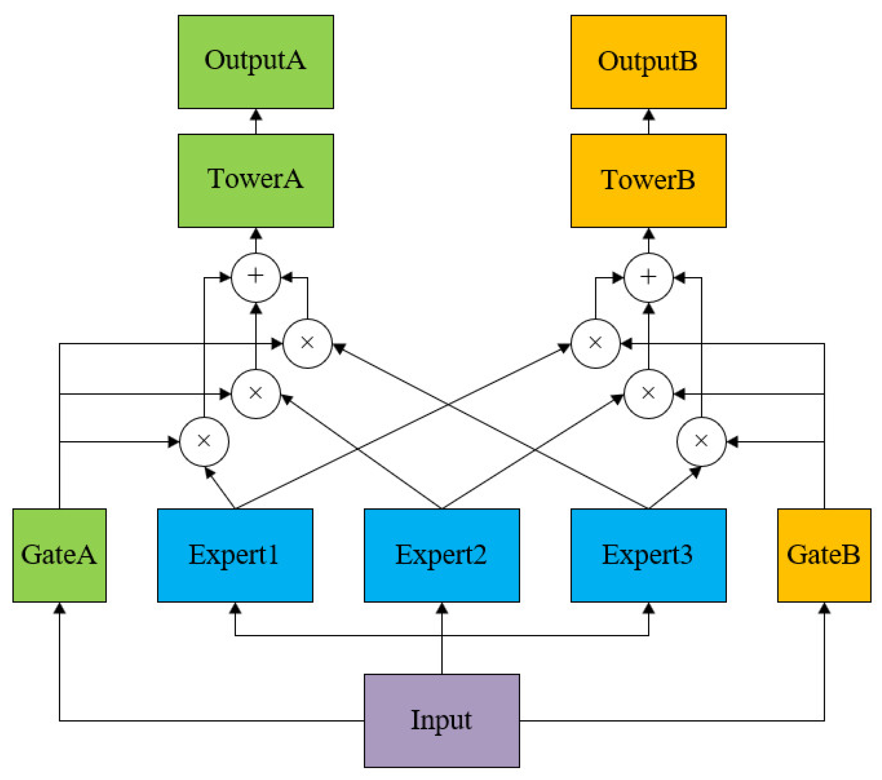
Unlike the MOE model, the MMoE model encompasses multiple gating networks, where each one is responsible for the output of a single task. There are common features among multiple tasks, as well as unique aspects for each one. The presence of multiple gating networks allows the MMoE model to better identify the differences between tasks while considering the correlation between them. Adding a separate gating network g^k for each task k, each output of task k can be formulated as follows:

$$y_k=h^k(f^k(x))$$

(2)

$$f^k(x)={\displaystyle \sum _{i=1}^n{g}^k{(x)}_i{f}_i(x)}$$

(3)

Moreover, the gating networks are simply linear transformations of the input using a softmax layer. They are expressed as follows:

$$g^k(x)=soft\max (W_{gk}x)$$

(4)

where $W_{gk}\in R^{n\times d}$ is a trainable matrix, $n$ represents the number of experts, and $d$ denotes the feature dimension. The MMoE network framework is shown in Figure 5.

2.2.2. MMoE-LSTM Network Model Framework

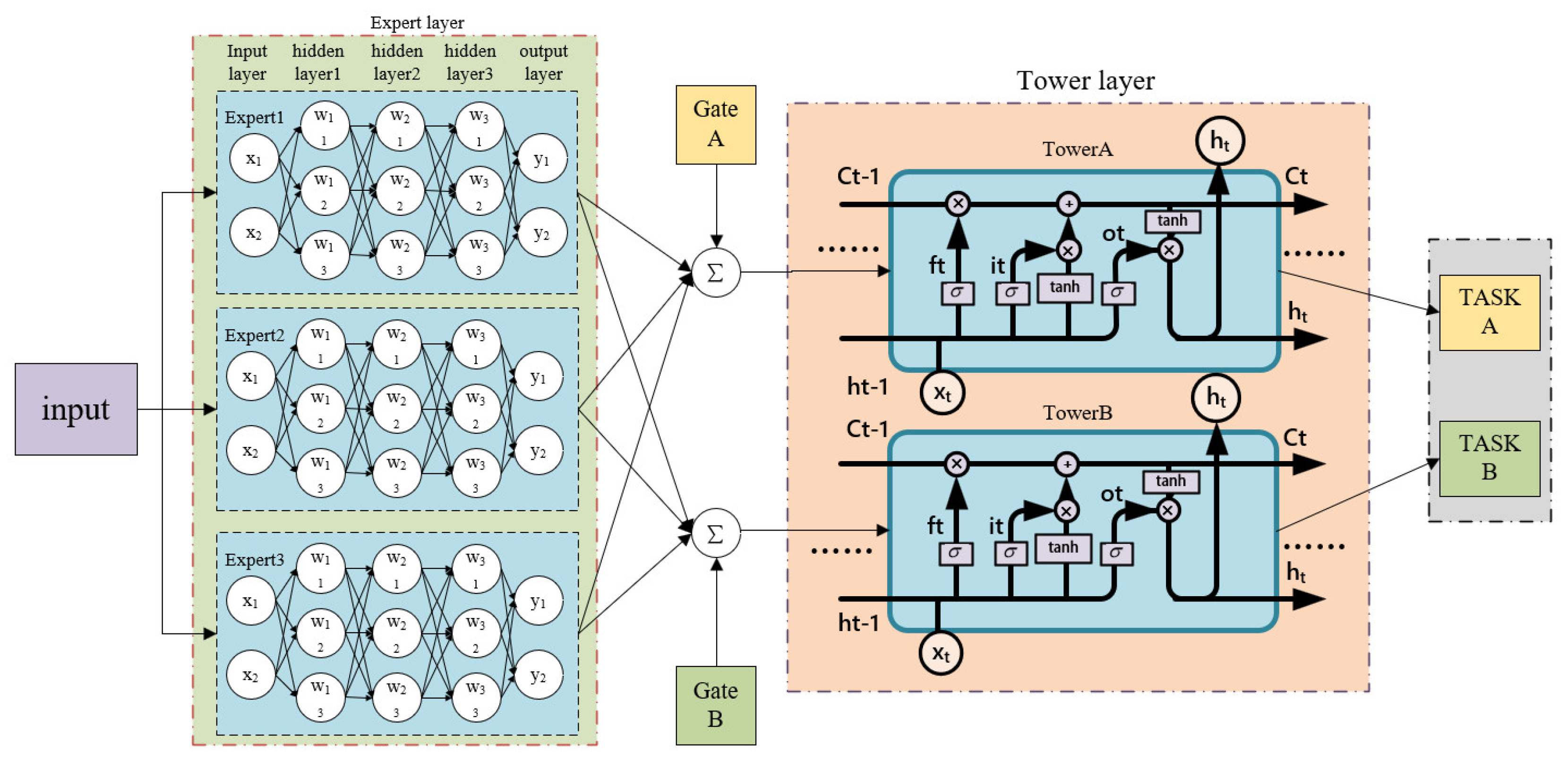
Unlike the MMoE network model framework, MMoE-LSTM sets the Expert neural network used to learn all aspects of data characteristics as MLPs. Unlike the single-hidden-layer neural network, MLP has multiple hidden layers, where each layer can introduce nonlinear transformation, and it has a stronger nonlinear modeling ability. The Tower layer fitting the output results of each task is replaced by LSTM from a single-hidden-layer neural network, which relies on LSTM’s unique gating mechanism to improve the ability of the Tower layer to deal with complex nonlinear features. The network model framework of MMoE-LSTM is shown in Figure 6.

Considering that the elastic support employs a hyper-elastic material like rubber, its performance data exhibit nonlinear and significant deformation characteristics in terms of stiffness and deformation. In such scenarios, the MLP, with its multi-hidden-layer structure, proves more effective than single-hidden-layer neural networks in capturing useful features from variable and nonlinear data. With its deep structure and gated mechanism, LSTM shows better effectiveness than fully connected neural networks in capturing the output data features of the Expert neural network. Therefore, compared to the traditional MMoE network framework, MMoE-LSTM can connect the memory and nonlinear modeling capabilities of LSTM networks to better identify the complex mechanical characteristics of elastic supports, thereby enhancing the model’s prediction effectiveness for elastic support performance data.

2.3. Multi-Task Loss Function Based on Coefficient of Variation Weighting and Ridge Regression

Multi-task learning models involve multiple loss functions, and during the training process, each task’s loss function is linearly weighted to derive the total loss function. The model’s training outcomes are highly sensitive to the weight coefficients assigned to each task’s loss function, necessitating considerable time for parameter tuning. When fusing the total loss function using a linear weighted method, challenges such as imbalanced loss decrease among different tasks and premature convergence of individual task loss functions may arise. To address these issues, this paper introduces the coefficient of variation weighting mechanism during the training process of the MMoE-LSTM model.

First, let’s define the coefficient of variation, also known as the relative standard deviation, as follows:

$$C_{it}={\sigma }_{it}/{\mu }_{it}$$

(5)

where $C_{it}$ represents the coefficient of variation for the i-th task at time step t, ${\sigma }_{it}$ denotes the standard deviation of the loss for the i-th task from generation 1 to t, and ${\mu }_{it}$ indicates the mean of the loss for the i-th task from generation 1 to t.

In this mechanism, the calculation of the loss for each task no longer relies solely on linear weighting to derive the total loss. Instead, the weight of each task’s loss in the total loss is determined by computing its coefficient of variation. The coefficient of variation represents the ratio of the standard deviation of each task’s loss to its mean, thereby reflecting the variability and uncertainty of the loss. A higher coefficient of variation for a task indicates greater fluctuation in its loss, implying that even minor changes in loss values could have a significant impact and may necessitate more attention and optimization relative to other tasks. Conversely, a task with a larger, stabilized loss value during training will be assigned a smaller weight.

The formula of variation for each task is as follows:

$$r_{it}=L_{it}/{\mu }_{it-1}$$

(6)

where $r_{it}$ represents the coefficient of variation for the i-th task at time step t, $L_{it}$ denotes the loss of task i at generation t, and ${\mu }_{it-1}$ indicates the average loss of task i from the first to the (t − 1)th generation.

Finally, the weight calculation formula for the loss of task i in the total loss at generation t is denoted as follows:

$$a_{it}=(C_{it}\times r_{it})/Z_t$$

(7)

where $Z_t$ represents the normalization factor, $Z_t=\sum _{i=1}^n(C_{it}\times r_{it}),$ and n is the total number of tasks.

Ridge regression, also known as L2 regularization, is a technique used during the training of a neural network model to mitigate the issue of weight explosion, where weight parameters become excessively large. This phenomenon can lead to issues such as gradient explosion and overfitting. L2 regularization addresses this by introducing a regularization penalty term to the total loss function, which helps control the size of the weight parameters. By adding this penalty term, L2 regularization helps prevent the occurrence of weight explosion, stabilizes the training process, and reduces overfitting. By constraining the weights of the network, this ensures that the model does not overly rely on any single feature or pattern within the training data, thereby improving the model’s ability to generalize to unseen data [40]. The formula for the penalty term of ridge regression is as follows:

$$l_{ridge}=\phi {\displaystyle \sum _{i=1}^p{\beta }_i^2}$$

(8)

In the formula, ${\beta }_i$ represents weight parameters in the model; $p$ represents the number of weight parameters; and $\phi$ highlights the regularization parameter, which controls the strength of regularization.

In the MMoE-LSTM model framework, there are multiple Expert neural networks, representing independent MLPs responsible for learning specific aspects of the input data. The introduction of ridge regression yields constraints that are placed on the weight parameters of these MLPs. The sum of squares of these weights, multiplied by a regularization parameter, is added to the total loss function; the result is considered as a loss term. This term limits the magnitude of the weights and helps in preventing issues such as weight explosion, overfitting, and gradient explosion.

In this work, the dynamic weighting mechanism, based on coefficient of variation weighting, is combined with the ridge regression penalty mechanism to constitute a new total loss function L. The ridge regression penalty term is also considered as an independent loss function. In casethe number of tasks is n − 1, the ridge regression penalty term is regarded as the n-th task, taking part in the weight value distribution calculation of the multi-task loss function. Therefore, the formula can be expressed as follows:

$$L(l_{1:n-1},a_{1:n},{\beta }_{1:p})={\displaystyle \sum _{i=1}^{n-1}(a_i}\times l_i)+a_n\phi {\displaystyle \sum _{i=1}^p{\beta }_i^2}$$

(9)

where $l_i$ is the loss of the i-th task, $a_i$ represents the dynamic weight coefficient of the i-th task loss, $n$ denotes the total number of tasks containing the ridge regression penalty item, $\phi$ indicates the regularization parameter, ${\beta }_i$ is the weight parameter of the Expert layer, and $p$ represents the number of Expert layer weight parameters.

Improving the loss function of multi-task learning models effectively resolves challenges such as imbalanced loss decrease, overfitting, and gradient explosion in multi-task learning. This enhancement strengthens the learning capability of the MMoE-LSTM model and improves predictive accuracy in multi-task networks. The parameters update of the whole network framework is based on Algorithm 1.

Algorithm 1. MMoE-LSTM optimization using multi-task loss function based on coefficient of variation weighting and ridge regression

Input: Training feature ${\mathit{x}}_{\mathbf{1}\mathit{:}\mathit{h}}$, regression label ${\mathit{y}}_{\mathbf{1}\mathit{:}\mathit{n}-\mathbf{1}}$, weight coefficients of initialized Expert layer ${\mathit{\beta }}_{\mathbf{1}\mathit{:}\mathit{p}}$, initialized task loss weight ${\mathit{a}}_{\mathbf{1}\mathit{:}\mathit{n}}$, Model initialization of network parameters $\mathit{W}$

Output: MMoE-LSTM parameters $\mathit{W}$

for each epoch t do In network model: $\mathrm{input}: {\mathit{x}}_{\mathbf{1}\mathit{:}\mathit{h}}$ $\mathrm{output}: {\widehat{y}}_{1:n-1},{\beta }_{i:p}=MMOE-LSTM(x_{1:h})$ In loss function model: $\mathrm{input}: {\widehat{\mathit{y}}}_{\mathbf{1}\mathit{:}\mathit{n}-\mathbf{1}}$, ${\mathit{y}}_{\mathbf{1}\mathit{:}\mathit{n}-\mathbf{1}}$$, {\mathit{\beta }}_{\mathbf{1}\mathit{:}\mathit{p}}$ $l_{1:n-1}=loss-fn({\widehat{y}}_{1:n-1},y_{1:n-1})$ $l_n=\phi {\displaystyle \sum _{i=1}^p{\beta }_i^2}$ $\mathrm{Update} {\mathit{a}}_{\mathbf{1}\mathit{:}\mathit{n}}$ $\mathrm{output}: L(l_{1:n-1},a_{1:n},{\beta }_{1:p})={\displaystyle \sum _{i=1}^n(a_i}\times l_i)$ $\mathrm{Update} \mathrm{model} \mathrm{parameters} \mathit{W}$ using Adam optimizer to find the minimum of $\mathit{L}\mathbf{(}{\mathit{l}}_{\mathbf{1}\mathbf{:}\mathit{n}-\mathbf{1}},{\mathit{a}}_{\mathbf{1}\mathit{:}\mathit{n}},{\mathit{\beta }}_{\mathbf{1}\mathit{:}\mathit{p}}\mathbf{)}$

end for

$\mathrm{return} \mathit{W}$

${\widehat{y}}_{1:n-1}$ represents the prediction result of the network model in the training process, whereas $loss-fn({\widehat{y}}_{1:n-1}$, $y_{1:n-1})$ consists of calculating the loss value for each task separately.

3. Experiment

This section discusses the generation of a dataset for studying the structural mechanical performance of the elastic supports of wind turbines, based on the digital twin model. The proposed method was validated experimentally using multiple datasets, showcasing its superiority over the existing techniques.

3.1. Data Generation

In this study, we validated the accuracy of the simulation results by conducting physical experiments. We examined the structural mechanical performance indicators of elastic supports across a range of structural design parameters using a digital twin model. Subsequently, we generated datasets for training network models.

3.1.1. Physical Test

This study centered on the elastic support of the generator in a 7 MW wind turbine, with a specific focus on conducting physical tests to measure its bidirectional static stiffness. To determine the rated load that each wind turbine elastic support must endure during normal working operations, we referenced the gravitational load necessary for testing the vertical static stiffness. This load is based on the performance parameters of the wind turbine, outlined in

Table 1. Wind-turbine-related parameters.

Parameter	Value
Wind turbine weight (t)	11.5
Number of elastic supports for assembly n	4
Rated speed (r/min)	1700
Rated input torque T(KN$·$m)	37.61
Distance between front and back elastic supports L(m)	1.6
Distance between left and right elastic supports B(m)	1.2

for reference.

The vertical gravitational load acting on each elastic support is defined as follows:

$$F_G=G/n$$

(10)

The vertical rated working load that each elastic support withstands is represented as follows:

$$F_{mean}=(T/2B)+(G/n)$$

(11)

According to Equation (11), the gravitational load that each elastic support needs to bear is determined as 28 kN, whereas the vertical rated working load is equal to 44 kN.

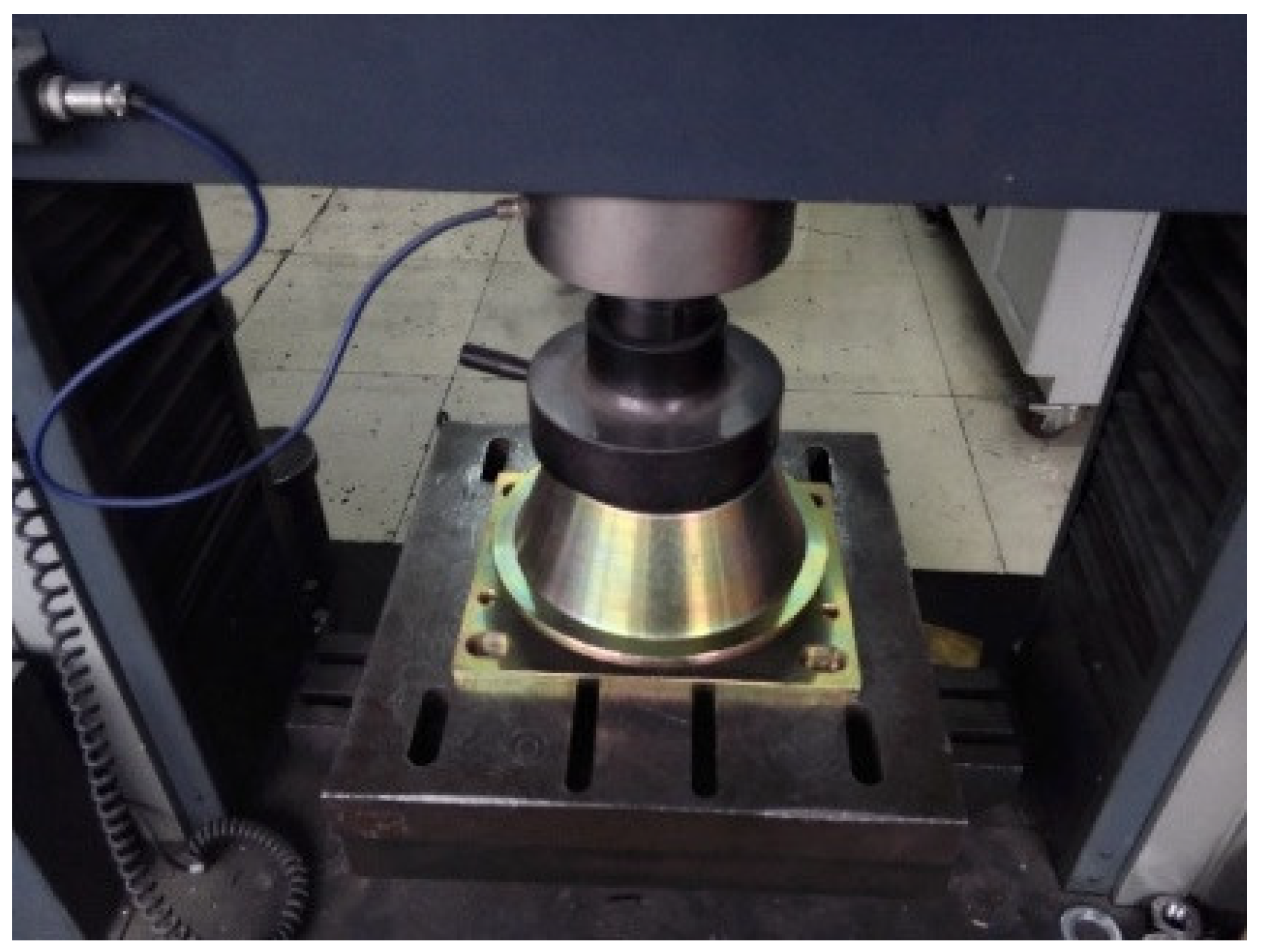
To test the static stiffness of the elastic support for a wind turbine generator, a microcomputer-controlled electro-hydraulic servo rubber testing machine, of model WXJ.200 (200 kN), is applied. The actual test is shown in Figure 7. The directional deformation occurring in the elastic support under various load values is measured to determine the bidirectional static stiffness of the overall structure of the elastic support.

The calculation method for static stiffness is as follows:

$$K=\frac{1.1F-0.9F}{S_2-S_1}$$

(12)

where F represents the measured load value, $S_2$ denotes the oriented displacement produced under 1.1 times the measured load, and $S_1$ represents the displacement produced under 0.9 times the measured load.

3.1.2. Three-Dimensional Model

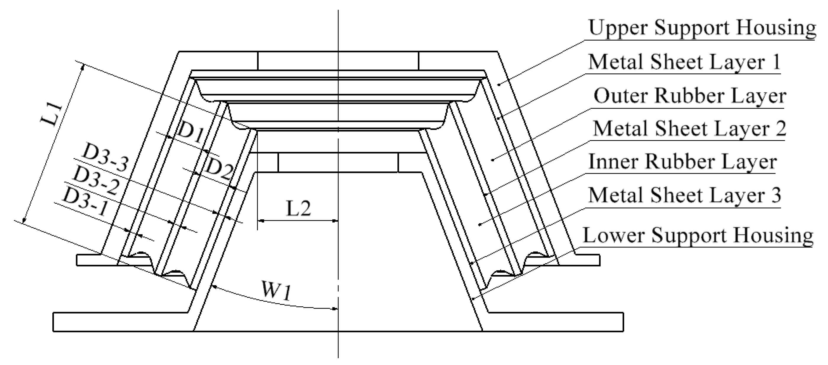
To construct a simulation model and conduct simulation calculations, it is imperative to initially create a three-dimensional model of the elastic support for the wind turbine. A simplified cross-sectional sketch of the wind turbine elastic support structure is depicted in Figure 8. This comprises a conical metal–rubber composite structure consisting of two layers of rubber, three layers of metal sheets, an upper support shell, and a lower support shell. Between the outer layer of rubber and the upper support shell, a layer of metal sheet 1 is installed. Additionally, between the two layers of rubber, metal sheet layer 2 acts as a separator. Similarly, between the lower support shell and the inner layer of rubber, metal sheet layer 3 is placed. The metal and rubber layers are connected by hot vulcanization, with each metal sheet layer possessing a uniform thickness.

The design parameters include outer rubber thickness D1, inner rubber thickness D2, metal sheet thickness D3, metal sheet length L1, inner metal sheet end radius L2, and taper W1. The ranges for these six design variables are provided in

Table 2. Design parameter value ranges.

Design Variable	Outer Rubber Thickness D1/mm	Inner Rubber Thickness D2/mm	Thickness of Iron Sheet D3/mm	Taper W1/(°)	Length of Iron Sheet L1/mm	Inner Iron Plate Port Radius L2/mm
Initial value	17	17	3	30	80	36
Upper limit value	20	20	5	36	100	40
Lower limit value	8	8	2	18	60	24

.

The elastic support was modeled parametrically using CAD software SOLIDWORKS (2022sp0.0). Subsequently, the three-dimensional model of the wind turbine elastic support was imported into the CAE software ANSYS WORKBENCH (2022R2) using the official CAD interfacing interface between SOLIDWORKS and ANSYS. This step prepared the model for subsequent simulation analysis.

3.1.3. Material Parameters

The wind turbine elastic support employs a rubber–metal composite vibration absorption mechanism, with the metal component crafted from QT345. Its specific material parameters are shown in

Table 3. QT345 material parameter table.

Material Property	Value
Density (kg/m3)	7850
Young’s modulus (GPa)	206
Poisson’s ratio	0.28
Yield stress (MPa)	345
Allowable stress (MPa)	230

. The rubber used is natural rubber with high hardness.

Note that the yield stress ${\sigma }_b$ is set to 345 MPa and the allowable stress [σ] is ${\sigma }_b/n$, where n represents the safety factor. When the safety factor is equal to 1.5, the allowable stress [σ] is set to 230 Mpa.

Rubber materials exhibit an extremely complex constitutive relationship, presenting significant challenges for the analysis of rubber products. Researchers have developed numerous rubber constitutive models through extensive theoretical analyses to describe their mechanical properties. Currently, the descriptive methods commonly used can be categorized into two main categories: the phenomenological description method, treating rubber as a continuous medium, and description based on statistical thermodynamics [41].

Based on phenomenological description, the strain energy density in the quadratic polynomial model can be expressed as follows:

$$U=f\left(I_1-3,I_2-3\right)+g\left(J-1\right)$$

(13)

Moreover, $g=\sum _{i=1}^N\frac{1}{D_i}{(J-1)}^{2i}$ and follows Taylor expansion, and then:

$$U={\displaystyle \sum _{i+j=1}^N{C}_{ij}}{\left(I_1-3\right)}^i{\left(I_2-3\right)}^j+{\displaystyle \sum _{i=1}^N\frac{1}{D_i}}{\left(J-1\right)}^{2i}$$

(14)

where $N$ represents the polynomial order, $C_{ij}$ denotes the material shear parameter, and the value of $D_i$ determines the compressibility of the material. It is worth noting that if all $D_i$ are null, the material is incompressible.

For the polynomial model, when $N=1$, one can obtain:

$${\mu }_0=2\left(C_{10}+C_{01}\right),k_0=2/D_1$$

(15)

$$\{\begin{array}{l}{I}_1={\lambda }_1^2+{\lambda }_2^2+{\lambda }_3^2\hfill \\ I_2={\lambda }_1^2{\lambda }_2^2+{\lambda }_1^2{\lambda }_3^2+{\lambda }_2^2{\lambda }_3^2\hfill \\ J={\lambda }_1^2{\lambda }_2^2{\lambda }_3^2\hfill \end{array}$$

(16)

where ${\mu }_0$ represents the initial shear modulus, $k_0$ indicates the initial bulk modulus, and ${\lambda }_1$, ${\lambda }_2,$ and ${\lambda }_3$ represent the three-directional principal stretches.

Moreover, when $N=1$, the expression for the complete polynomial, only employing terms of degree one, transforms into the strain energy expression of the Mooney–Rivlin model [42]. It is expressed as follows:

$$U=C_{10}\left(I_1-3\right)+C_{01}\left(I_2-3\right)+\frac{1}{D_1}{\left(J-1\right)}^2$$

(17)

Under normal operating conditions, the strain experienced by the wind turbine’s elastic support is relatively small. The Mooney–Rivlin model is known for effectively capturing the mechanical properties of rubber materials under conditions of small strain and is also considered the simplest among the existing rubber constitutive models. Therefore, the Mooney–Rivlin model was chosen as the constitutive model for the rubber material in the elastic support of a wind turbine, to be utilized in subsequent simulation calculations.

In the material library of ANSYS WORKBENCH, the Mooney–Rivlin model was utilized to characterize the rubber material. According to the data provided by the manufacturer of the elastic support, the parameters of the constitutive model were as shown in

Table 4. Constitutive model parameters.

Rubber Hardness	C10/MPa	C01/MPa	D1
50	0.3744	0.00936	0
60	0.4947	0.0139	0
65	0.59238	0.1481	0

.

3.1.4. Static Analysis and Mesh Independency Verification

The bidirectional stiffness and stress distribution of the elastic support under rated working conditions were simulated and tested using the static mechanics module of ANSYS WORKBENCH. The accuracy of these simulation results relies heavily on the mesh generation of the grid model, necessitating a verification of mesh independence.

The model is meshed using tetrahedral elements, and various meshes with different scales are constructed to illustrate the influence of mesh size and quantity on the simulation results. The multiple simulation results are depicted in

Table 5. Influence of different mesh sizes on simulation results.

Mesh Software	ANSYS WORKBENCH (2022R2)
Grid elements	44,340	50,488	58,990	78,896	109,834	161,394	304,545
Grid size/mm	10	9	8	7	6	5	4
Equivalent stress of rubber parts/Mpa	2.2629	2.3212	2.3646	2.4287	2.4632	2.4792	2.5026
Vertical deformation/mm	6.4438	6.5385	6.6812	6.7893	6.8742	6.9154	6.9362
Transverse deformation/mm	7.2563	7.3426	7.4581	7.5685	7.6132	7.6893	7.7246

.

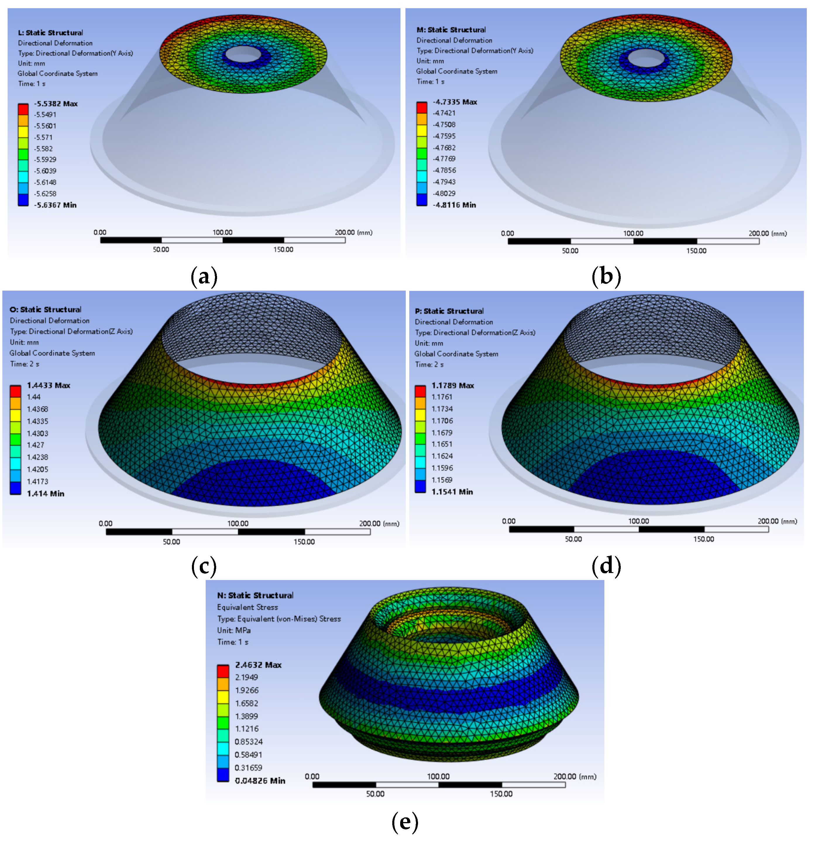
As shown in Table 5, when the mesh size is less than or equal to 6 mm and the number of mesh elements exceeds 109,834, further refinement of the mesh size results in simulation result changes of less than 2% across multiple simulations. Moreover, the average mesh quality exceeds 0.8. Considering the trade-off between simulation computational time and accuracy, a mesh size of 6 mm was selected. The partial simulation results are shown in Figure 9.

In Figure 9, the average vertical displacement of the top surface of the elastic support is utilized to evaluate the overall vertical static stiffness of the elastic support, while the average horizontal displacement of the outer shell of the elastic support side is employed for assessing the displacement of the overall lateral static stiffness of the elastic support. According to the static stiffness calculation Equation (11), the vertical static stiffness obtained from the simulation is 6.87 KN/mm and the lateral static stiffness is 7.61 KN/mm.

To calculate the error between the simulation test results and the real test results, the calculation formula is as follows:

$$E=\frac{\left|R_{exp}-R_{sim}\right|}{R_{exp}}\times 100\%$$

(18)

where $E$ represents the numerical error, $R_{exp}$ represents the physical test result, and $R_{sim}$ represents the simulation test result.

According to the error calculation formula, the numerical error between the vertical static stiffness levels obtained by simulation and a real test is 7.41%, and for lateral static stiffness, the error is 5.69%. As such, the numerical errors between the finite element simulation results and the physical experiment findings are both within 10%, indicating the reliability of the finite element simulation results.

3.1.5. Digital Twin Model Verification Experiment

To further validate the reliability of the digital twin model of the wind turbine elastic support, verification tests were conducted. The dimensions and material properties of the digital twin model were modified according to another type of elastic support.

Physical tests showed that this type of elastic support under a vertical load of 50 KN has a vertical static stiffness of 6.1 KN/mm, while under a vertical preload of 30 KN and a lateral load of 10 KN, the lateral static stiffness is 7.8 KN/mm.

Through simulation tests to simulate actual working conditions, the results were measured, as shown in Figure 10.

According to the simulation results, the vertical static stiffness (obtained from the simulation calculation) is 6.61 KN/mm, with an error of 8.36% compared to the physical test results. The lateral static stiffness is 8.24 KN/mm, with an error of 5.64% compared to the physical test results. As such, the errors between the data generated by the digital twin model and the data obtained from the physical test are within 10%, which verifies that after modifying the structural and material parameters of the digital twin model, the generated data still conform to the physical test results. This proves that the digital twin model can effectively generate data that meet the physical characteristics of the wind turbine elastic support, and we can surmise that the data generated by the digital twin model have a guaranteed accuracy.

If there are significant errors between the simulation data and the physical test data, these errors may be due to unreasonable simplifications during the construction of the digital twin model, incorrect definitions of material parameters, unreasonable mesh division of the model, or other such reasons. To improve the reliability of the digital twin model, it is necessary to adjust the geometric features, mesh shape, mesh size, and other details of the digital twin model according to the existing physical model and test results, to ensure that the simulation data generated based on the digital twin model can effectively describe the physical characteristics of the wind turbine elastic support.

3.1.6. Experimental Design

The experiment was carried out using the Latin hypercube sampling (LHS) method. Referring to Table 2, six structural design parameters are listed as input parameters, whereas the vertical static stiffness K₁, the lateral static stiffness K₂, the maximum stress σ₁ on the rubber part, and the mass M₁ of the rubber part represent the output parameters. A total of 200 design points were selected for simulation experiments, resulting in the generation of two datasets. The dataset using rubber material with a shore hardness of 50 is named dataset 1, while the one using rubber material with a shore hardness of 60 is named dataset 2. Partial data can be found in

Table 6. Part of dataset 1 (rubber hardness 50).

	Design Variable						Performance Index
	D1/ mm	D2/ mm	D3/ mm	W1/(°)	L1/ mm	L2/ mm	K1/ KN/mm	K2/ KN/mm	σ1/ MPa	M1/ kg
1	76.53	12.57	19.57	4.69	38.43	21.17	4.29	9.84	5.05	1.08
2	99.73	15.87	18.61	4.59	34.36	26.61	8.60	12.25	1.67	1.64
3	88.96	14.74	14.73	4.67	35.75	23.47	7.94	14.94	2.22	1.18
4	97.34	8.46	10.58	2.04	27.29	22.02	20.54	40.86	2.22	0.66
…	…	…	…	…	…	…	…	…	…	…
199	63.73	10.07	10.38	2.81	27.35	24.17	8.48	14.24	7.06	0.41
200	87.76	18.02	19.61	4.77	34.51	31.72	7.24	7.07	1.87	1.56

and

Table 7. Part of dataset 2 (rubber hardness 60).

	Design Variable						Performance Index
	D1/ mm	D2/ Mm	D3/ mm	W1/(°)	L1/ mm	L2/ mm	K1/ KN/mm	K2/ KN/mm	σ1/ MPa	M1/ kg
1	67.04	18.71	13.13	2.41	31.16	30.86	7.53	7.59	3.17	0.79
2	69.52	17.51	11.87	3.55	29.48	19.64	4.95	12.44	4.07	0.72
3	63.78	15.77	14.36	3.46	39.38	28.49	7.65	9.65	2.76	0.80
4	74.93	13.82	10.19	4.80	25.73	34.08	19.55	15.78	2.12	0.66
…	…	…	…	…	…	…	…	…	…	…
199	87.02	19.71	19.50	4.22	32.79	30.58	8.74	9.29	1.76	1.55
200	96.97	13.21	17.04	2.82	33.73	18.87	8.73	23.88	2.384	1.23

.

3.2. Data Processing and Evaluation Index

In this section of the study, two datasets generated from physical-based simulation models were preprocessed to meet the requirements of the network model training. The data consisted of six structural design parameters as input parameters and four structural performance indicators as output parameters.

Considering that the scales of the input and output parameters are distinct, to avoid issues related to instability in training, slow convergence, and poor training results, caused by the large differences between feature values, the dataset was normalized to obtain all parameters on the same scale. The mathematical formula for data normalization is as follows:

$$x_n=\frac{X_n-X_{\min }}{X_{\max }-X_{\min }}$$

(19)

where x_n represents the value of the n-th item in a dataset after normalization, X_n denotes the value of the n-th item in a dataset before normalization, X_max is the maximum value in the dataset before normalization, and X_min is the minimum value in the dataset before normalization.

The preprocessed dataset is shuffled and then partitioned into a training set and a validation set using the 3:1 ratio. The training set is employed for subsequent training of the network model, while the validation set is utilized to evaluate the predictive accuracy of the network model, rather than as training data for the network model.

To evaluate the superiority of the proposed method, the mean squared error (MSE) and the coefficient of determination R2 (R-squared) are used to evaluate the prediction results of the network model. They are expressed as follows:

$$MSE=\frac{1}{N_P}{\displaystyle \sum _{i=1}^{N_P}{(y_i-{\widehat{y}}_i)}^2}$$

(20)

$$R\text{-}squared=\frac{{\displaystyle \sum _{i=1}^{N_P}{({\widehat{y}}_i-y_{mean})}^2}}{{\displaystyle \sum _{i=1}^{N_P}{(y_i-y_{mean})}^2}}$$

(21)

where ${\widehat{y}}_i$ represents the predicted value, $y_i$ denotes the true value, $y_{mean}$ indicates the average of the true values, and $N_P$ represents the sample size.

3.3. Comparative Experiment of Multi-Model Based on Small Sample Dataset

The network models were developed using the open-source PyTorch (2.0.0) framework. The network input comprised six variables, all of which were design parameters of the elastic support structure. The neural network needed to learn four tasks simultaneously to achieve multi-task learning. Task 1 involves the mass of the rubber material used in the elastic support structure, Task 2 focuses on predicting the vertical static stiffness, Task 3 focuses on the lateral static stiffness, and Task 4 is on the maximum stress on the rubber part under the rated operating condition. These tasks represent various structural mechanics performance indicators.

Both the MMoE and MMoE-LSTM network frameworks contain five Expert networks, four Tower networks, and four gated networks. The Expert networks in MMoE-LSTM are all multi-layer perceptron with three hidden layers, containing 13, 27, and 13 neurons, respectively, in each hidden layer, and the activation function of the hidden layers is ReLU. The Tower networks are LSTM, with 13 neurons in the LSTM layer and two other layers. The output is fit through a linear layer. The Expert networks and Tower networks in MMoE are single-hidden-layer fully connected neural networks, with 13 neurons in the hidden layer; finally, the activation function of the hidden layer is ReLU.

The MLP, PLE, and Cross-Stitch Networks (CSNs) are employed for comparison. The MLP structure is simple, and in terms of multi-task learning, it uses typical hard parameter sharing. In this experiment, its structure consists of three hidden layers, with 13, 27, and 13 neurons, respectively, in each hidden layer, and the activation function of the hidden layer is ReLU. As for PLE, it has the same parameter settings for Expert and Tower networks as MMoE, with three common experts based on the common experts, where each task has a unique expert. Finally, the CSN contains four MLPs, each of which contains three hidden layers, with 13, 27, and 13 neurons, respectively, in each hidden layer, and the activation function of the hidden layer is ReLU. There are cross-connection layers between each multi-layer perceptron, suitable to achieve cross-integration of feature representations between the different tasks.

Moreover, MSE is used as the loss function for each task, and the Adam optimizer is applied for optimization, with a learning rate set to 0.001 and a training period set to 400.

A total of five experiments were conducted, using MLP, PLE, CSN, MMoE, and MMoE-LSTM network frameworks. After training, the results for the predictive abilities of all five models on the validation dataset were obtained, as shown in

Table 8. The final loss value and coefficients of determination of each neural network model.

Dataset	Task	MLP		PLE		CSN		MMoE		MMoE−LSTM
		MSE	R2	MSE	R2	MSE	R2	MSE	R2	MSE	R2
Dataset 1	1	8.9 × 10−3	0.9127	6.2 × 10−3	0.9532	9.6 × 10−3	0.9361	1.2 × 10−3	0.9649	1.4 × 10−4	0.9947
	2	1.2 × 10−2	0.8563	6.8 × 10−4	0.9341	7.3 × 10−4	0.9382	1.6 × 10−3	0.9265	1.9 × 10−4	0.9795
	3	8.2 × 10−2	0.8732	7.6 × 10−4	0.8965	9.7 × 10−4	0.8794	1.3 × 10−3	0.8692	2.5 × 10−4	0.9763
	4	8.9 × 10−3	0.7467	2.3 × 10−3	0.8072	7.3 × 10−3	0.7536	5.6 × 10−3	0.7730	3.4 × 10−3	0.8509
Dataset 2	1	6.3 × 10−3	0.9371	6.2 × 10−4	0.9849	2.4 × 10−3	0.9572	8.3 × 10−4	0.9781	8.7 × 10−4	0.9791
	2	8.4 × 10−3	0.8729	4.6 × 10−4	0.9629	8.6 × 10−4	0.9359	6.1 × 10−4	0.9432	1.9 × 10−4	0.9781
	3	1.3 × 10−3	0.8947	8.1 × 10−4	0.9163	1.2 × 10−3	0.9037	9.2 × 10−4	0.9094	4.5 × 10−4	0.9731
	4	7.2 × 10−3	0.7925	2.9 × 10−3	0.8397	3.5 × 10−3	0.8164	3.7 × 10−3	0.8143	2.4 × 10−3	0.8932

.

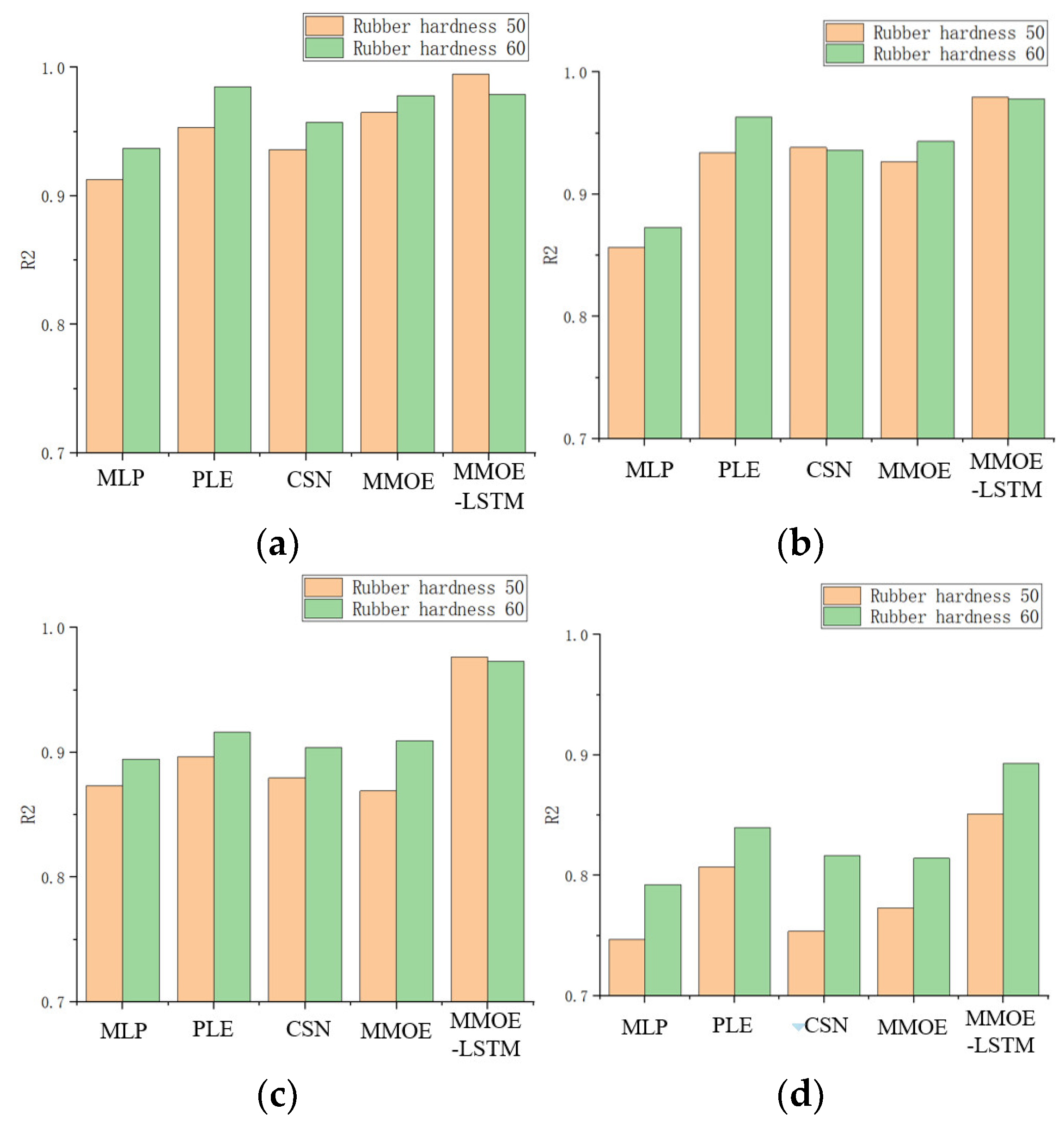
Under the same training conditions, a comparison of the predictive accuracy of each model for the four tasks was performed, and the results are illustrated in Figure 11.

The training results shown in Table 8 highlight that, under the same training conditions, the multi-task learning model MLP, employing hard parameter sharing, has the worst overall predictive ability for multiple task objectives. Meanwhile, although soft parameter sharing multi-task learning models MMoE, PLE, and CSN perform better than MLP, they still struggle in accurately capturing the complex patterns and extracting features from the data in small sample cases. Consequently, the predictive accuracy for individual tasks is poor, and the loss values for some tasks converge early during the training process.

Compared to the traditional MMoE network framework, the MMoE-LSTM can more efficiently learn the patterns and features in the data of structural mechanical performance indicators under small sample conditions. The predictive ability of the model for multiple task objectives is significantly improved; yet, there is still an issue concerning premature convergence of individual task losses and imbalanced loss decrease among tasks during the training process.

Referring to the results in Figure 11, the predictive accuracy for task 4 is not high for all models, with the loss value for task 4 only reaching a magnitude of 1 × 10⁻³, while the loss values for other tasks reach a magnitude of 1 × 10⁻⁴. This suggests that there is a poor correlation between task 4 and the other tasks; furthermore, the multi-task learning network models also have a poor predictive accuracy for this task. Even with enhancements at the level of the network structure, this problem is not resolved.

3.4. Comparative Experiment of Multi-Task Loss Function Optimization

Although the MMoE-LSTM network framework exhibits a superior performance compared to other network frameworks on both datasets, the predictive accuracy for tasks with poor correlations remains low. To address this issue, this study employed a dynamic loss weighting approach based on the coefficient of variation weighting and ridge regression, rather than employing a linear weighted method to fuse loss functions in the MMoE-LSTM model framework. This approach was then compared to other methods for fusing multi-task loss functions on the dataset of elastic support structure mechanics performance indicators. After finishing the training, the predictive capabilities of the network models, trained using various methods on the validation dataset, were as displayed in

Table 9. The final loss value and coefficients of determination of each multi-task loss function fusion method.

Dataset	Task	Uncertainty Weighting		Geometric Loss		Scaled Loss Approximate Weighting		COV−L2
		MSE	R2	MSE	R2	MSE	R2	MSE	R2
Dataset 1	1	2.7 × 10−4	0.9932	7.2 × 10−3	0.9437	5.6 × 10−3	0.9846	2.9 × 10−4	0.9929
	2	6.9 × 10−4	0.9386	1.6 × 10−3	0.9251	4.3 × 10−4	0.9686	4.4 × 10−4	0.9618
	3	6.7 × 10−4	0.9334	8.4 × 10−4	0.9037	5.1 × 10−4	0.9598	2.9 × 10−4	0.9721
	4	2.2 × 10−3	0.9109	2.8 × 10−3	0.8967	2.3 × 10−3	0.9186	5.1 × 10−4	0.9577
Dataset 2	1	2.3 × 10−4	0.9936	4.7 × 10−3	0.9477	1.2 × 10−3	0.9659	3.1 × 10−4	0.9917
	2	2.1 × 10−3	0.9138	5.9 × 10−4	0.9583	5.7 × 10−4	0.9506	2.9 × 10−4	0.9642
	3	3.9 × 10−4	0.9582	3.7 × 10−4	0.9820	6.3 × 10−4	0.9619	4.3 × 10−4	0.9758
	4	2.1 × 10−3	0.9125	2.6 × 10−3	0.8993	1.9 × 10−3	0.9204	5.0 × 10−4	0.9601

.

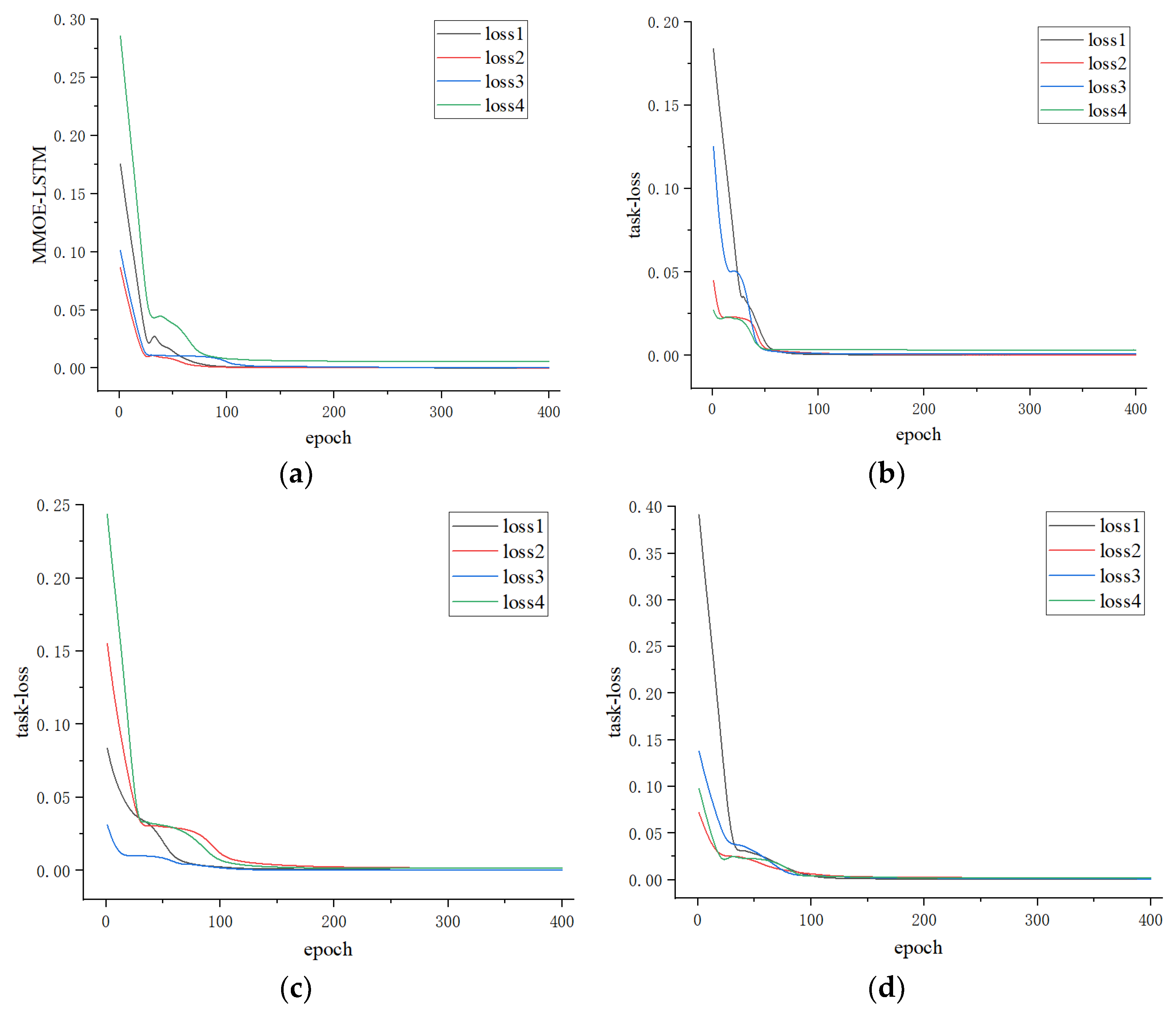
Under the same network framework (MMoE-LSTM) and parameter settings, the loss function optimization method proposed in this study outperforms other multi-task loss function optimization methods when being applied on both datasets. After optimizing the loss function, although the MMoE-LSTM model does not fully outperform the un-optimized model in predicting all four tasks, it successfully tackles the problem of premature convergence of individual task loss functions and imbalanced loss decrease between tasks due to the poor correlation between tasks. Therefore, the loss of each task reaches a magnitude of 1 × 10⁻⁴. A comparison chart is given in Figure 12. Compared to the use of the proposed loss function optimization method during the MMoE-LSTM model training process, the loss functions of the four tasks have all decreased to a lower level, without encountering the problem of premature convergence of a single task’s loss function due to poor correlation between individual tasks.

4. Conclusions

This study enhances the network framework of the MMoE model and the method for fitting the multi-task total loss function, achieving multi-objective prediction of the mechanical PIS of wind turbine elastic supports using small sample datasets.

First, a digital twin model was constructed based on a physical model, and the results of the physical experiment were compared with the results of a simulation experiment. The error between the simulation and the physical experiment was less than 10%, which verified the reliability of the digital twin model. Based on these comparisons, the Latin hypercube method was applied for the experimental design, and a large amount of data reflecting the relationship between structural design parameters and mechanical PIs was generated through simulation, avoiding the high costs of physical tests and providing a reliable data source for subsequent network model training.

Moreover, in order to further improve the learning energy of a multi-task prediction model on complex nonlinear data, this study improved MMoE-LSTM based on MMoE. Under the same training conditions, the MMoE-LSTM prediction model achieved an improvement of 0.03 to 0.1 in the R2 value for multiple tasks compared to other multi-task prediction models. The experimental results indicate that the MMoE-LSTM prediction model is better equipped to handle the nonlinear characteristics of elastic supports as reflected in structural mechanical PIs, such as stiffness and stress.

To address the issue of uneven loss decreases among tasks in multi-task learning, this study combined the dynamic weighting mechanism based on coefficient of variation weighting with the ridge regression penalty mechanism to form a new multi-task loss function optimization method. On the basis of the MMoE-LSTM prediction model, the multi-task loss function optimization method proposed in this study was employed. The experimental results showed that the MSE loss values of each task decreased to a 1 × 10⁻⁴ magnitude, eliminating the issue of premature convergence of individual task loss values. Under the same training conditions, compared to other multi-task loss function optimization methods, the MMoE-LSTM prediction model utilizing the optimization method proposed in this study demonstrated a comprehensive superiority in terms of the R2 values and MSE loss values for multiple tasks.

The experimental results indicate that using the method proposed in this study to fit the multi-task total loss function can effectively address the issues of premature convergence of individual task loss functions and imbalanced loss decrease across multiple tasks. These issues are caused by several factors including limited data, a low correlation between tasks, and strong nonlinear characteristics of the data. Additionally, the proposed method outperforms other approaches in terms of effectiveness.

The method proposed in this study can achieve multi-objective prediction of the mechanical PIs of wind turbine elastic supports at a low cost, providing guidance for new product development.