Validation of Ecology and Energy Parameters of Diesel Exhausts Using Different Fuel Mixtures, Consisting of Hydrogenated Vegetable Oil and Diesel Fuels, Presented at Real Market: Approaches Using Artificial Neural Network for Large-Scale Predictions

Abstract

Machine learning models have been used to precisely forecast emissions from diesel engines, specifically examining the impact of various fuel types (HVO10, HVO 30, HVO40, HVO50) on the accuracy of emission forecasts. The research has revealed that models with different numbers of perceptrons had greater initial error rates, which subsequently reached a stable state after further training. Additionally, the research has revealed that augmenting the proportion of Hydrogenated Vegetable Oil (HVO) resulted in the enhanced precision of emission predictions. The use of visual data representations, such as histograms and scatter plots, yielded significant insights into the model’s versatility across different fuel types. The discovery of these results is vital for enhancing engine performance and fulfilling environmental regulations. This study highlights the capacity of machine learning in monitoring the environment and controlling engines and proposes further investigation into enhancing models and making real-time predictive adjustments. The novelty of the research is based on the determination of the input interface (a sufficient amount of input parameters, including chemical as well as technical), which characterizes the different regimes of the diesel engine. The novelty of the methodology is based on the selection of a suitable ANN type and architecture, which allows us to predict the required parameters for a wide range of input intervals (different types of mixtures consisting of HVO and pure diesel, different loads, different RPMs, etc.).

1. Introduction

It is well-known that diesel engines are needed in our society for several reasons [1,2]. The main important reason is the high thermal efficiency of fuel energy conversion to mechanical energy compared to other types of engines [3,4]. Heavy machinery, shipping, long-distance transportation, and agricultural machinery could be titled as the very successful examples of adaptation in society [5,6,7]. Great versatility can be realized, as diesel engines can run on a variety of fuels, including biodiesel and renewable diesels, such as HVO (Hydrogenated Vegetable Oil) [8]. Due to that, flexibility and the potential to reduce environmental impact occur. HVOs generally emit fewer greenhouse gases and pollutants compared to conventional diesel, improve air quality, and reduce environmental impact. HVO can be used in existing diesel engines without requiring any modifications, making it a convenient choice for fleet operators and consumers searching to reduce their carbon footprint without investing in new vehicles or equipment [9,10].

However, different diesel engine modes are related to different combustion processes, which generate unpredictable emissions [11,12]. The ability to use empirical formulas to create distributions of predicted emissions (smoke, CO, NOx, etc.) is, in many cases, unproductive due to the uncertainty of the initial conditions. The use of an artificial neural network for predictions and estimations makes it possible to solve a complex task.

(a)

It allows for acquiring and merging a broader and more varied collection of training data to assess if the enhanced dataset can mitigate the initial high error rates and accommodate the intricacy of the neural network models.

(b)

It allows for performing trials to determine the ideal equilibrium between the quantity of perceptrons in the hidden layers and the extent of training to reduce the likelihood of overfitting and to establish a steady error rate.

(c)

It expands the scope of fuel types in the trials by including different kinds of fuel, such as HVO10 to HVO50, to thoroughly evaluate their influence on the accuracy of emission predictions.

(d)

It allows for devising and executing a set of experiments to further investigate the machine learning model’s capacity to adapt predictions according to the fuel type, with a specific emphasis on regional and regulatory discrepancies.

(e)

It can be used to create advanced visualization tools to effectively demonstrate the distribution and precision of emission forecasts across various fuel types, hence improving the comprehensibility of the data.

(f)

It can be used to conduct cross-validation experiments utilizing supplementary datasets to verify the dependability and uniformity of the prediction model, thus guaranteeing its resilience when applied to various data inputs.

(g)

It can be used to conduct research of longer durations to observe the effectiveness and precision of the model in real-life situations and investigate the incorporation of real-time data for dynamic prediction and improvement.

(h)

It can be used to examine the possible advantages and difficulties of using advanced neural network structures, such as deep learning or convolutional neural networks, to forecast diesel engine emissions.

The implementation of predictive control approaches represents a notable advancement in the optimization of internal combustion engines (ICEs), which are inherently intricate and nonlinear systems.

Generally, it is very difficult to relate the ecological parameters of diesel engines to technological parameters of fuel and engine behavior. Due to origin of experimental data (complex task, chaotic nature), traditional self-regulation procedures for data are necessary (statistical filters, partial fitting of dependencies, etc.) We decided to use a non-traditional approach to ANN after the training procedure can predict the output parameters with high precision. The novelty of the research is based on the determination of the input interface (sufficient amount of input parameters, including chemical as well as technical), which characterizes the different regimes of the diesel engine.

The novelty of the methodology is based on the selection of a suitable ANN type and architecture, which allows us to predict the required parameters from a wide range of input intervals (different types of mixtures consisting of HVO and pure diesel, different loads, different RPMs, etc.). The architecture of ANNs (single hidden layer, number of perceptrons, shape of nonlinear function) is tightly related to establishing the nonlinear relationship between inputs and outputs (learning procedure), and this routine, as a “state-of-art” technology, could be titled as a technological novelty for technical predictions.

Predictive control plays one of the most important roles in the driving of the machine learning processes. ICEs and virtual sensors for fault detection systems are powerful tools for continuous control and rapid prediction of deviations from averaged values. Generally, control of exhaust could be presented under the supervision of presented systems. Hoang [13] presented a review paper that evaluated the structure and applicability of the artificial neural networks (ANNs) model, comparing predicted results with experimental data. ANNs have emerged as a promising approach to predict engine performance and exhaust emissions in biodiesel-fueled diesel engines. The ANN model demonstrated a high determination coefficient, achieving an accuracy of over 95% in predicting engine behaviors based on trained, tested, and validated data. Norouzi et al. [14] reviewed the application of Model Predictive Control (MPC) for ICEs and analyzed recent developments in MPC and AI-ML-MPC for ICE control applications. ICEs are complex, nonlinear systems with operational limits like emissions, noise, and actuator constraints. Optimizing ICEs requires extensive experimentation and costly calibration of the Engine Control Module (ECM). MPC methods have shown promising results for real-time optimal control. Ricci et al. [15] analyzed the integration of virtual sensors into on-board control systems, assessing the potential of advanced machine learning technologies to replace physical sensors. The control of internal combustion engines is becoming increasingly challenging due to increasing performance and emission regulations. Machine learning techniques, such as virtual sensors and fault detection systems, are being used in the automotive field for real-time and low-cost implementation. The LSTM + One-Dimensional Convolutional Neural Networks (1DCNNs) architecture, which combines Long Short-Term Memory (LSTM) with 1DCNN, has proven promising for signal analysis. Kwak et al. [16] used ANN to predict the frequency and amplitude of combustion instability. Experimental data from a CH₄-fueled combustor were used to train the ANN model. The study found that the equivalence ratio, axial flame distance, and injection velocity varied the frequency and amplitude of combustion instability. The ANN trained using three input parameters accurately predicted both frequency and amplitude, confirming the importance of these parameters. Anand et al. [17] predicted the efficiency and NOx emission of a spark ignition engine using the ANN model, originally proposed for real-time computations in electronic control units. A two-zone, quasi-dimensional thermodynamic simulation of a four-stroke SI engine fueled with biogas was conducted. The model predicted the combustion and emission characteristics of biogas, revealing that carbon dioxide can reduce NOx emissions, but lower cylinder pressures reduce engine power and thermal efficiency. Hanuschkin et al. [18] investigated cycle-to-cycle variations in a four-stroke direct-injection spark-ignition gasoline engine using high-speed scanning particle image velocimetry and in-cylinder pressure measurements. Binary classifiers predicted high-indicated mean effective pressure combustion cycles based on in-cylinder flow features and engineered tumble features. The results were independent of machine learning methods and robust to hyper-parameter selection.

ANNs have become a fundamental tool [19] in predictive analysis for assessing engine performance and environmental effects. ANNs are used in many applications to forecast outcomes and show their adaptability and precision in improving operational efficiency and tackling environmental issues in the automotive and energy industries [20,21]. Böyükdipi et al. [22] investigated the impact of ammonia (NH₃) as a fuel additive on engine vibration parameters in sunflower biodiesel. Ammonia was blended into sunflower biodiesel at varying ratios and combusted under no-load conditions. Vibration data were recorded and analyzed using ANN models. The results showed that the ammonia additive in sunflower biodiesel negatively affected engine vibration. The accuracy rates of the ANN models were 99.206%, 99.675%, and 99.505%. Wang et al. [23] described an application of adaptive neural network modeling and MPC for engine simulation. A radial basis function neural network was used to model crankshaft speed, intake manifold pressure, and manifold temperature. The reduced Hessian method was implemented for nonlinear optimization in MPC, making it suitable for internal combustion engines. Park et al. [24] studied gas turbine combustor operating characteristics using real-time data from industrial gas turbines. Input parameters included Turbine Exhaust Temperature (TET) and major design parameters. The predictive neural network structure was optimized, with an average predicted Root Mean Square Error (RMSE) below 0.02296. The mean TET had the highest accuracy, but sudden changes in operation could increase the prediction error. Peak errors occurred at start-up and shutdown processes. Park et al. [25] used ANN to detect faults in large-scale industrial gas turbines. ANN predicted fuel injection characteristics, preventing frequent operating failures during start-up procedures. Data from GE 7FA gas turbines were used, and the method could detect overheating that started before OP4. A sensitivity analysis of the gas turbine’s operating characteristics for each nozzle was performed to identify fuel supply system problems and advance nozzle system abnormalities. Ziółkowski et al. [26] used artificial neural networks to analyze fuel consumption in motor vehicles and human impact on the environment, focusing on passenger cars. A database of 1750 vehicles was used to train the neural networks, with the MLP 22-10-3 network selected. The model’s predictions were analyzed using linear Pearson correlation coefficients and coefficients of determination. A reduced number of neurons was built, and the model’s ex post prediction errors were evaluated. The tool is intended for designing passenger cars with internal combustion engines, providing a more accurate prediction of fuel consumption. Nejadmalayeri et al. [27] used sparse experimental data and URANS simulation results, demonstrating their effectiveness in predicting in-cylinder pressure profiles. Low-cetane-number fuels increase misfire risk in diesel engines. To mitigate this, an ignition assistant and a reliable engine-control system are needed. Traditional training data collection is time-consuming and expensive. A data-driven model was developed to predict average cylinder pressure, varying cetane number, main injection timing, and ignition assistant power. Jadidi et al. [28] analyzed the soot formation in combustion systems, which is a growing concern due to their environmental and health effects. Despite the complexity of soot evolution, most industrial device simulations neglect or approximate it due to high computational costs. The study used a supervised ANN technique to accurately predict soot concentration fields in ethylene/air laminar diffusion flames with low computational cost. The network performed well in both training scenarios and new flames, with relatively low integrated error. Zhang et al. [29] identified four types of oscillating combustion in industrial gases based on various factors, such as intrinsic mixing, kinetics, heat loss interaction, single inflowing fluctuation, inflowing fluctuation superposition, and fuel switching. The study analyzed these types using unsteady perfectly stirred reactor combustion models and chemical explosive mode analysis. Short-term and long-term prediction models were established using NARMAX and neural network methods, providing validation and data support for controller and actuator design.

Si et al. [30] presented a sophisticated DRG-CSP-ANN method as a joint method combining a Directed Relation Graph (DRG), Computational Singular Perturbation (CSP), and ANN to develop a new skeletal mechanism for methane MILD combustion. The reduced mechanism, Reduced-ANN, simplifies the detailed GRI-3.0 mechanism to 13 species and 35 reactions, outperforming other skeletal mechanisms. The method reduces errors in predicting autoignition time and flame propagation speed, making it a promising method for mechanism reduction.

Deep Convolutional Neural Networks (DNNs) have revolutionized turbulent combustion simulations and automotive engine design. By surpassing the challenges of physical modeling, they offer fresh perspectives on the multidimensional aspects of these problems. Rinav et al. [31] used DNN to estimate nitrogen oxide (NOx) emissions in heavy-duty vehicles. The approach used variables from two datasets, an engine dynamometer and a chassis dynamometer, to predict NOx emissions. The models had high accuracy, with R² scores above 0.99 for both models on cold/hot Federal Test Procedure and Ramped Mode Cycle data. The models had a mean absolute error percentage of approximately 1%, comparable to physical NOx emission measurement analyzers. DNN NOx emissions models can also be effective tools for fault detection in Selective Catalytic Reduction systems. Warey et al. [32] created a model that can be used as an emissions prediction sub-model in the Virtual Engine Model framework, thus reducing computational costs. Analysis-driven pre-calibration of modern automotive engines is crucial for reducing hardware investments and accelerating engine designs. Advanced modeling tools like the Virtual Engine Model (VEM) use Computational Fluid Dynamics (CFD) to streamline the calibration process. However, accurate predictions of emissions, particularly carbon monoxide, hydel, and smoke, remain a challenge. A machine learning approach was used to correlate in-cylinder images with engine-out emissions, resulting in improved predictions and qualitative trends. Johnson et al. [33] used a machine learning approach to correlate in-cylinder images of early flame kernel development in a spark-ignited gasoline engine with flame propagation. High-speed images were captured for 357 cycles, and three models were trained: a linear regression model, a Deep Convolutional Neural Network (CNN), and a CNN built with assisted learning. The study found that early flame images provided information for regression and CNN models, but limitations exist due to complex thermal physics. Future research should consider increasing training data or introducing additional measurements. Owoyele et al. [34] used the deep artificial neural networks to replace lookup tables in tabulated combustion models. The grouped multi-target artificial neural network was introduced, allowing for accurate capture of flame liftoff, autoignition, and other quantitative trends. The approach was validated using an n-dodecane spray flame and methyl decanoate combustion in a compression ignition engine. The use of neural networks in conjunction with the grouping mechanism reduces memory footprint and computational costs, allowing for higher-fidelity engine simulations with detailed mechanisms. Mondal et al. [35] used the deep neural network trained on inexpensive experiments to predict unstable operating conditions in a swirl-stabilized combustor. The intermittent operation of fossil fuel power plants and the unpredictable availability of renewable energy sources present new challenges to suppressing high-amplitude pressure oscillations, such as Thermoacoustic Instabilities (TAIs), which can lead to performance degradation and system failures. Predicting these instabilities is crucial for combustion system design and operation. Data-driven approaches have shown success in predicting instability maps, but limited data are often needed for practical combustion systems. Wang et al. [36] analyzed the engine exhaust emissions, and modeling was provided using radial basis function neural networks (RBFNNs) to predict engine performance under various working conditions. The model used various input parameters, including engine speed, load, fuel flow rate, air mass flow rate, scavenge air pressure, maximum injection pressure, electronic parameters, and environmental conditions. The results showed that the R² = 0.984, with smaller mean % errors.

The conclusions of the literature review can be presented as follows. ANNs are used by many researchers for the determination of unknown engine parameters. ANN is one of the most advanced methods of engine mode parameter simulation. As one of the best realizations of ANN for technical purposes, the feedforward neural network allows for training based on proven engine modes and therefore simulates new, yet unknown, modes. The ecological aspect is very important here, because the determination of waste concentrations takes place virtually with high accuracy. Technical parameters of ANN (number of hidden layers, number of perceptrons in the hidden layer, optimal number of input/output units) are under question and depend on the tested situation.

Feedforward neural networks are useful for prediction tasks because they can learn complex data relationships, and accurate predictions are based on input features. Three important reasons are significant: ANN as a universal approximator, the applicability of ANN, and nonlinearity. Based on the Universal Approximation Theorem, feedforward neural networks with one hidden layer with enough neurons can fit any continuous function with arbitrary precision. ANNs can adapt to different types of data and tasks by adjusting their architecture, activation functions, and other parameters. Feedforward neural networks can model nonlinear relationships between input and output variables. This flexibility allows them to capture complex data patterns that linear models cannot.

2. Materials and Methods

The energy and environmental performance of the engine was investigated using a compression ignition (CI) engine and special measuring equipment, the layout of which is shown in Figure 1. The main technical characteristics of the engine are presented in

Table 1. The main technical characteristics of the CI engine.

Parameter	Value
Number of cylinders	4/OHC
Displacement	1.9 dm3
Bore	79.5 mm
Stroke	95.5 mm
Compression ratio	19.5
Power	66 kW (at 4000 rpm)
Torque	180 Nm (at 2000–2500 rpm)
Filling of cylinders with air	Turbocharger
Fuel injection	Direct injection

, and the main characteristics of the test equipment are presented in

Table 2. The main characteristics of internal combustion engine test equipment.

Equipment	Measurement Range	Accuracy
Engine load bench KI-5543	0–440 Nm	±1.2 Nm
Electronic fuel scales SK-5000	0–5000 g	±1.0 g
Air mass meter BOSCH HFM 5	8–370 kg/h	±2%
Temperature sensor (K-type thermocouple)	0–1200 °C	±1.5 °C
SOI matavimo įranga VAG-Com	0–20 CAD bTDC	±1.0° CAD
Exhaust gas analyzer AVL DiCom 4000
Volumetric CO2 concentration	0–20%	±0.1%
Volumetric CO concentration	0–10%	±0.01%
Volumetric CH concentration	0–20,000 ppm	±1 ppm
Volumetric NOx concentration	0–5000 ppm	±1 ppm
Volumetric O2 concentration	0–25%	±0.01%
Smokiness (opacity)	0–99.99%	±0.01%

. This equipment enabled us to control the engine speed and load, measure the fuel and air consumption, evaluate the exhaust gas composition, and measure the temperature and pressure at various points in the engine. The engine’s electronic control system controls the fuel injection strategy, the turbocharger performance, and exhaust gas regeneration, and we could adjust the control algorithms of these devices accordingly.

During the experimental tests, the engine was operated at various speeds and loads. The power system of the engine was controlled in two ways: 1—by means of an electronic control unit (ECU) and 2—by means of an additional adjustment of the Start of Injection (SOI) of the fuel and the Exhaust Gas Recirculation (EGR). This extended the limits of the engine control algorithm stored in the ECU memory and set the engine performance over a wider range of the fueling system control. Fuel injection was adjusted by adjusting the SOI from 2 Crank Angle Degree before Top Dead Centre (CAD bTDC) to 1 CAD bTDC. The EGR ratio was adjustable from 0 to 0.45. The engine was tested in seven stages, and details of the engine’s operating conditions and control details at each stage are shown in Figure 2. Only stationary states are presented in our experiment, without intermediate time-dependent states. In Figure 2, showing the Brake Thermal Efficiency (BTE) of an engine, we can see the seven stages of the test carried out with the engine running at different loads and speeds and at different SOI and EGR adjustments. Ten parameters for validation of ANN prediction were used in our simulation (see

Table 3. The physico-chemical properties of the fuel blends.

Properties	HVO10	HVO30	HVO40	HVO50
Kinematic viscosity at 40 °C, cSt	3.802	3.149	3.034	3.000
Dynamic viscosity, mPa · s	3.125	2.550	2.451	2.365
Density at 15 °C, g/mL	0.822	0.810	0.808	0.793
Cold filter plugging point, °C	−12	−27	−28	−34
Pour point °C	−39	−40	−42	−45
Flash point, °C	90.0	90.0	75.2	63.9
Water content, % V/V	0.0031	0.0025	0.0023	0.0021
Cetane number	54.5	58.1	59.6	59.9
C/H ratio	6.69	6.46	6.34	6.22
Stoichiometric air to fuel ratio, kg air/1 kg fuel	14.56	14.67	14.73	14.79
Lower heating value (LHV), MJ/kg	42.67	42.83	42.92	43.13

and

Table 4. Experimental parameters of diesel engine used for an ANN as the input parameters.

Cluster	Index	Abbr.	Parameter	Units	Interval
					XMIN	XMAX
1	0	P10	$\mathrm{The} \mathrm{excess} \mathrm{air} \mathrm{ratio} \left(\mathit{\lambda }\right)$	-	1.0	10.0
1	1	P03	Brake mean effective pressure (BMEP)	MPa	0.0	1.2
1	2	P02	EGR ratio	-	0.0	0.5
1	3	P11	Start of Injection (SOI)	CA bTDC	−3.0	18.0
2	4	P09	Cetane number	-	5.0	85.0
1	5	P01	Engine speed (n)	rpm	800.0	4000.0
2	6	P04	Volume fraction of HVO100	%	0.0	100.0
2	7	P05	Volume fraction of D100	%	0.0	100.0
2	8	P12	C/H ratio	-	5.0	7.0
2	9	P06	$\mathrm{Stoichiometric} \mathrm{air} \mathrm{to} \mathrm{fuel} \mathrm{ratio} ({\mathit{l}}_{\mathbf{0}}$)	1 kg of air/1 kg of fuel	10.0	20.0
2	10	P08	Lower heating value (LHV)	MJ·kg−1	18.0	60.0
2	11	P07	Density	kg·m−3	600.0	900.0

). One of the presented parameters, BTE (R02), was used for the explanation of the different regimes (stages) of the diesel engine. Parameter R02 is presented in two forms, experimental value R02 and, simulated by ANN, value R02*, which is the subject of the following discussion. Parameter RolNo on the x-axis represents a technical experimental number that plays a role in enumeration only.

During the experiment, engine performance was measured when the engine was running on different blends of pure diesel (D100) and HVO (HVO100). These fuel blends were purchased from a petrol station at different times of the year (summer, autumn, and winter), and the HVO concentration in the fuel blends was 30% (HVO30), 40% (HVO40), and 50% (HVO50), respectively. Fuel dealers use certain additives to maintain the mixed fuel’s stability. The HVO10 fuel blend was created by thoroughly combining the fuel components in a container for a duration of 2–3 min. Throughout the testing procedure, fuel mixture stability was maintained by redirecting a portion of the fuel flow from the fuel pump and injectors back to the fuel tank. This allowed for a continuous mixing process to occur, as shown in Figure 1. A blend of 10% HVO with diesel (HVO10) was prepared using pure D100 and HVO100 fuels. The physico-chemical properties of all of the fuel blends used in the experiments were tested in the laboratory and are shown in Table 3.

The tests were repeated 5 or more times with the engine running in different modes for fuel blends with different HVO concentrations. The wide range of tests allowed us to assess the dependence of the engine’s energy and environmental performance on the fuel composition, the engine’s operating conditions, and the control algorithm. The energy efficiency of different fuel blends was assessed according to the brake-specific fuel consumption (BSFC) and the Brake Thermal Efficiency (BTE). The ecological performance was assessed by measuring the concentration of carbon dioxide (CO₂) in the exhaust gases and calculating the specific emissions of CO₂ (SCO₂), as well as the concentration of oxygen (O₂), the specific emissions of carbon monoxide (SCO), the specific emissions of unburned hydrocarbons (SCH), the concentration of NOx, and the specific emissions of NOx (SNOx), and by presenting the measured smokiness.

3. Simulation Setup

3.1. Data Collection

The performance of ANNs is highly dependent on the ANN architecture and the dynamic training mode. Three different stages (amount of input layer, number of perceptrons in the hidden layer, number of hidden layers, amount of output layer) are described in previous work [37]. Clusterization of input/output data according to similar or related properties allows for decreasing the random fluctuations of the total network error (TNE). We decided to create the first input cluster according to the technical conditions (P10, P03, P02, P11, P01) and the second input cluster according to the burning chemistry suggestions (P09, P04, P05, P12, P06, P08, P07) (see Table 4). This assumption (grouping or clusterization) allows for significantly improving the ANN learning process and avoiding unpredictable increases in the TNE. For the output, three clusters were created: one for volumetric O₂ concentration (R08), SNO_x (R04), and volumetric concentration of NO_x (R09); a second for smoke (R00), brake-specific fuel consumption (BSFC) (R01), and Brake Thermal Efficiency (BTE) (R02); and a third for SHC (R05), SCO (R03), volumetric CO₂ concentration (R07), and SCO₂ (R06) (see

Table 5. Experimental parameters of diesel engine used for ANN as the output parameters.

Cluster	Index	Abbr.	Parameter	Units	Interval
					YMIN	YMAX
1	7	R08	Volumetric O2 concentration	%	0.5	20.0
1	8	R04	SNOx	g·kWh−1	0.1	20.0
1	9	R09	Volumetric NOx concentration	ppm	10.0	10,000.0
2	3	R00	Smokiness	m−1	0.001	100.0
2	4	R01	Brake-specific fuel consumption (BSFC)	g·kWh−1	150.0	3000.0
2	5	R02	Brake Thermal Efficiency (BTE)	-	0.01	0.5
3	6	R05	SHC	g·kWh−1	0.01	2.0
3	0	R03	SCO	g·kWh−1	0.5	10.0
3	1	R07	Volumetric CO2 concentration	%	0.1	15.0
3	2	R06	SCO2	g·kWh−1	100.0	2000.0

).

3.2. Simulation Routine

Figure 3 represents the schema of the realized ANN in the framework of VALLUM01 [38]. Due to adjusting possibilities, bias was included in the hidden layer. The programmed package VALLUM01, which contains a graphical, user-friendly interface for input, output, and control, was created using the JAVA Eclipse framework, version: 2021-12 (4.22.0)). For ANNs, two typical classes from [39] were used: matrix and neural network. As an S-shaped function, a sigmoidal function was used:

$$\sigma \left(x\right)=\frac{1}{1+e^{-x}}$$

(1)

An ANN consists of an input layer, with the number of units L = 12 (yellow), a single hidden layer, with the number of perceptrons M = 100,000,000 (blue), and an output layer, with the number of units N = 10 (green). Normalization/denormalization plugins were used for conversion/deconversion of any real value (pink) from the requested interval into the (0; 1) interval. Information flow was directed from bottom to top.

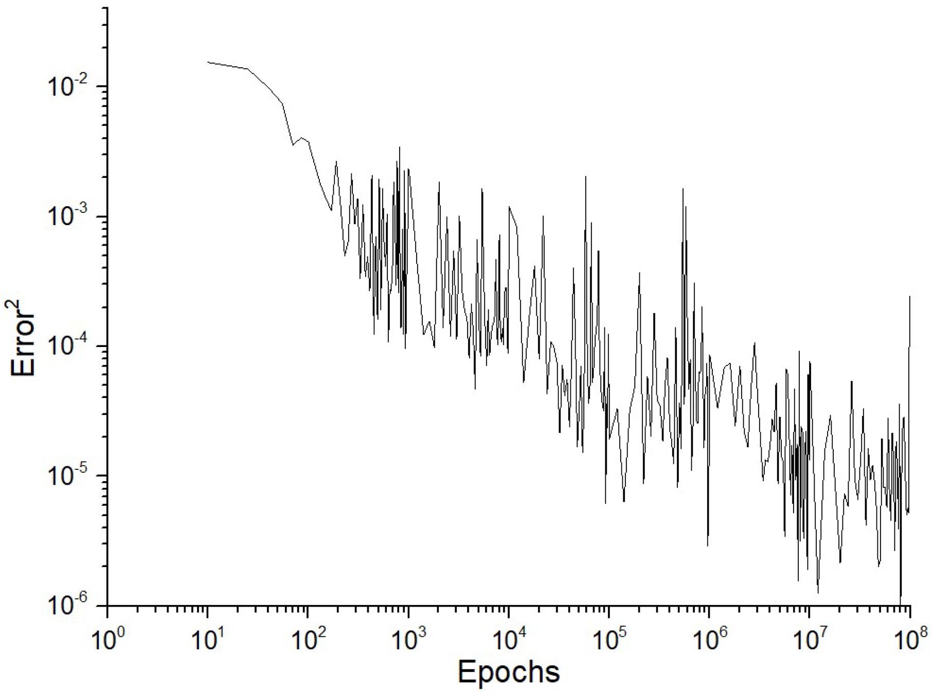
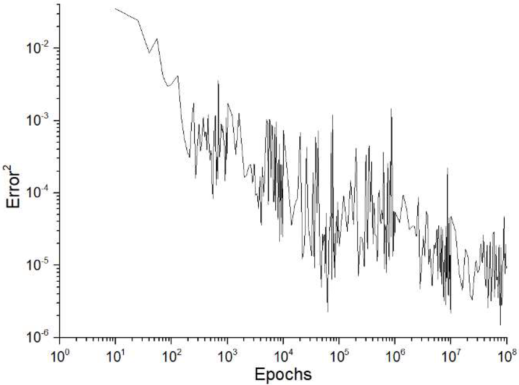
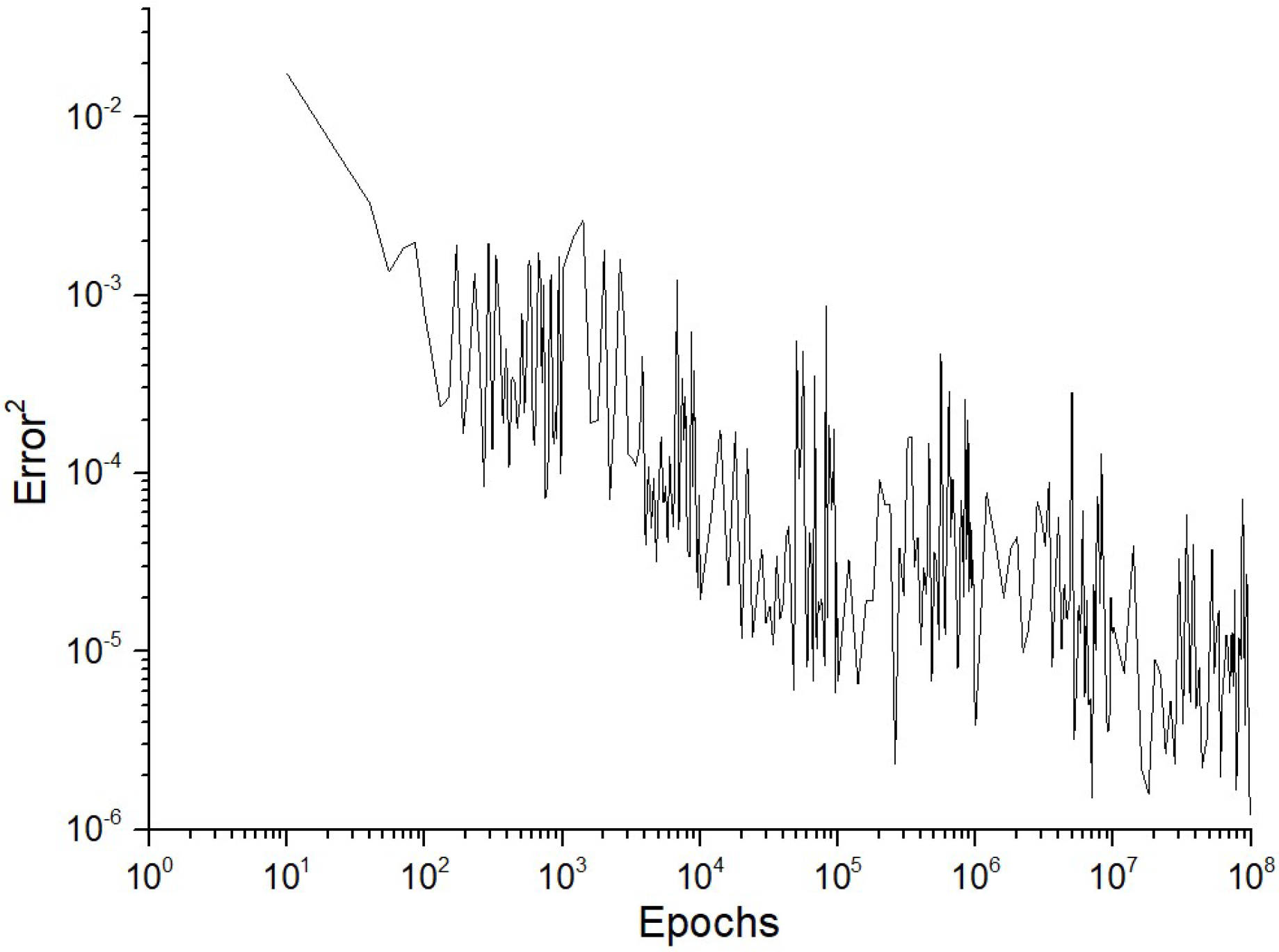
4. Results

Table 6. The procedure of training and validation of ANNs. Input layer L = 12, output layer N = 10, amount of perceptron in the hidden layer M, learning rate 0.01.

Project	One Hidden Layer	Training					Validation
Name	M	Routine	File	Events	Epochs	TNE2	File	Events
T50	50	T7	50-10304050.csv	717	100,000,000	Table 7-1
T100	100	T8	100-10304050.csv	717	100,000,000	Table 7-2
T200	200	T9	200-10304050.csv	717	100,000,000	Table 7-3
10	100		100-10304050.csv				10.csv	164
30	100		100-10304050.csv				30.csv	166
40	100		100-10304050.csv				40.csv	213
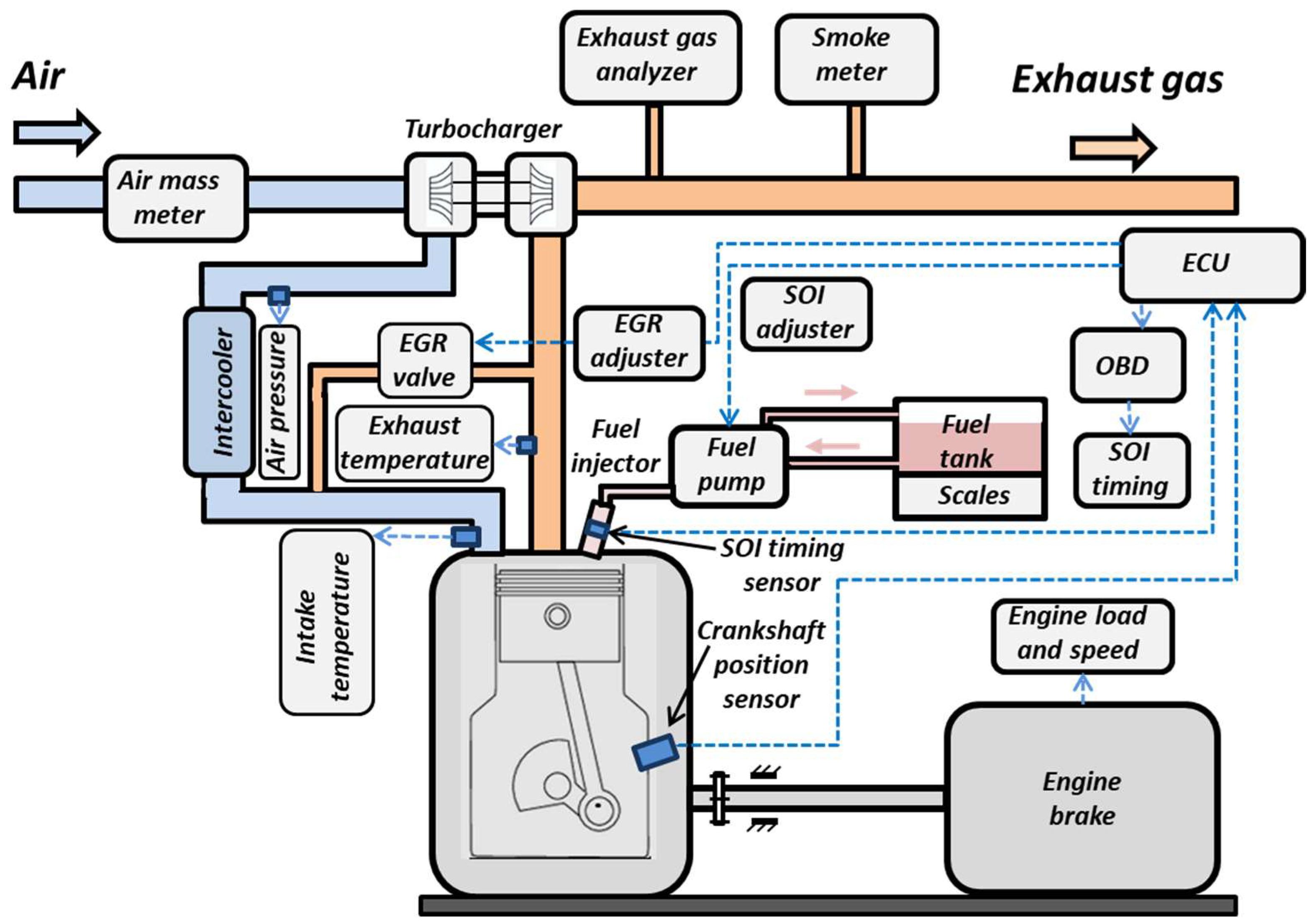
50	100		100-10304050.csv				50.csv	174

describes the provided procedures for training and validation of ANNs. In this case, the parameters are presented according to the notations in Figure 3. Initially, the training data file was formed from files 10.csv, 30.csv, 40.csv, and 50.csv without any selection, and all records were included. Finally, the number of events of the training file 10304050.csv was distinguished to be 717 (164 + 166 + 213 + 174). The training procedure was provided using 100,000,000 epochs for ANN consisting of a single hidden layer containing M = 50, M = 100, and M = 200 perceptrons (three separate training projects T50, T100, T200). Then, for the validation procedure, separate files, 10.csv, 30.csv, 40.csv, and 50.csv, were used in the prediction regime using only one training stamp, 100-10304050.

Table 7. TNE² dependence on epochs number. Evolution of the ANN training. Number of events, 717. Number of epochs, 100,000,000.

Number of Perceptrons in the Single Hidden Layer
M = 50
M = 100
M = 200

seems to depict the error rate of a machine learning model during its training phase across a certain number of iterations, known as epochs. There are three distinct plots that correspond to three different training regimes. These regimes are distinguished by the “number of perceptrons in the single hidden layer” of a neural network, which are M = 50, M = 100, and M = 200. Each figure exhibits a consistent decline, suggesting that as the number of epochs grows, the square of error rate TNE² typically decreases. The observed result is anticipated as the neural network acquires knowledge from the training data gradually, modifying its weights to minimize the total network error.

The variations in the error rate indicate that the training process encounters some variability, which may be attributed to certain variables, such as the data’s complexity, the learning pace, or the existence of noisy data.

When comparing the three graphs, it is not immediately evident if increasing the number of perceptrons in the hidden layer has a substantial effect on the pace at which convergence occurs or the stability of the error rate. Nevertheless, there seems to be a pattern in which the plots with a greater number of perceptrons (M = 100 and M = 200) exhibit an initially higher error rate but thereafter demonstrate a more consistent drop compared to the M = 50 plot.

Without precise mistake rate numbers, it is impossible to measure the extent of progress in error reduction. Nevertheless, it seems that as the network grows in complexity (with an increased number of perceptrons), the initial error also increases, indicating the possibility of overfitting or the need for more epochs to achieve a similar decrease in error.

Essentially, Table 6 illustrates how the quantity of perceptrons in a single hidden layer impacts the learning procedure of a neural network. Nevertheless, in the absence of further context or quantitative data, it is difficult to make definitive inferences about the efficacy of any system.

Table 8. R01 parameter dependence on fuel type.

Fuel	Parameter	Distributions of Predicted Value
HVO10
HVO30
HVO40
HVO50

,

Table 9. R02 parameter dependence on fuel type.

Fuel	Parameter	Distributions of Predicted Value
HVO10
HVO30
HVO40
HVO50

,

Table 10. R07 parameter dependence on fuel type.

Fuel	Parameter	Distributions of Predicted Value
HVO10
HVO30
HVO40
HVO50

,

Table 11. R06 parameter dependence on fuel type.

Fuel	Parameter	Distributions of Predicted Value
HVO10
HVO30
HVO40
HVO50

,

Table 12. R08 parameter dependence on fuel type.

Fuel	Parameter	Distributions of Predicted Value
HVO10
HVO30
HVO40
HVO50

,

Table 13. R03 parameter dependence on fuel type.

Fuel	Parameter	Distributions of Predicted Value
HVO10
HVO30
HVO40
HVO50

,

Table 14. R05 parameter dependence on fuel type.

Fuel	Parameter	Distributions of Predicted Value
HVO10
HVO30
HVO40
HVO50

,

Table 15. R09 parameter dependence on fuel type.

Fuel	Parameter	Distributions of Predicted Value
HVO10
HVO30
HVO40
HVO50

,

Table 16. R04 parameter dependence on fuel type.

Fuel	Parameter	Distributions of Predicted Value
HVO10
HVO30
HVO40
HVO50

and

Table 17. R00 parameter dependence on fuel type.

Fuel	Parameter	Distributions of Predicted Value
HVO10
HVO30
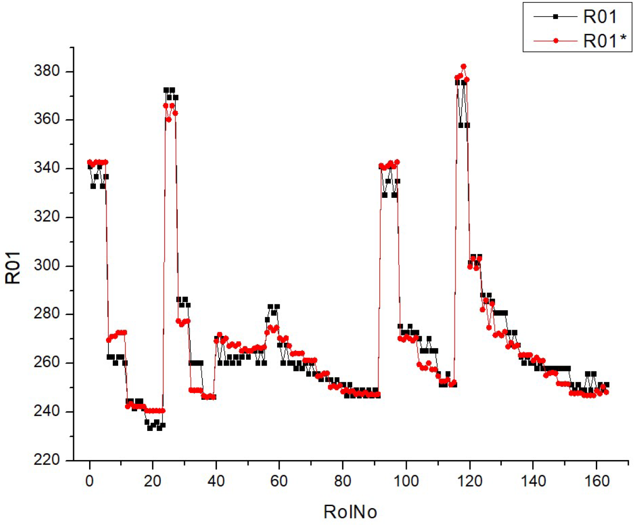
HVO40
HVO50

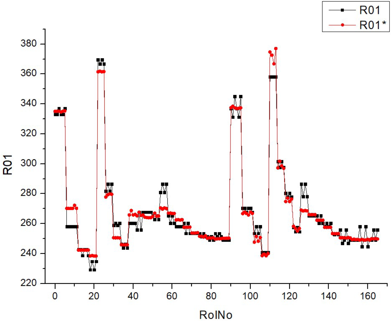
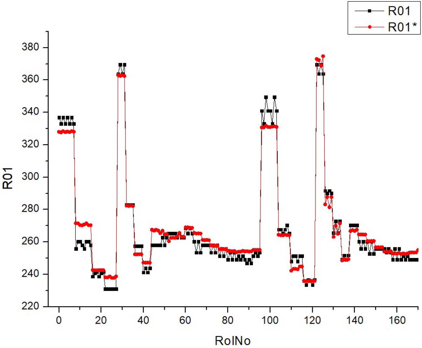
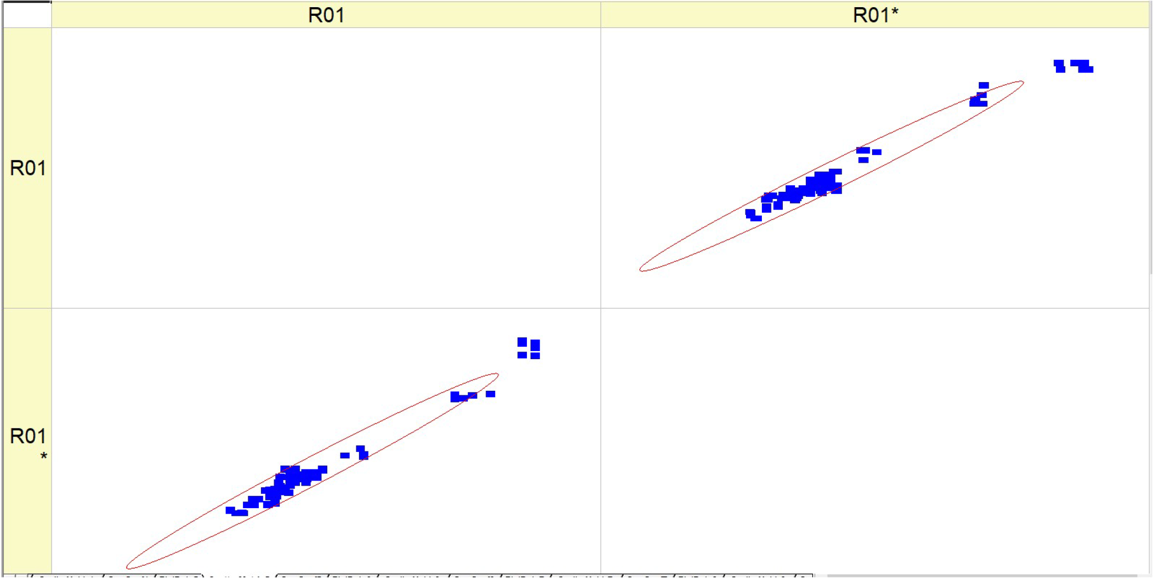
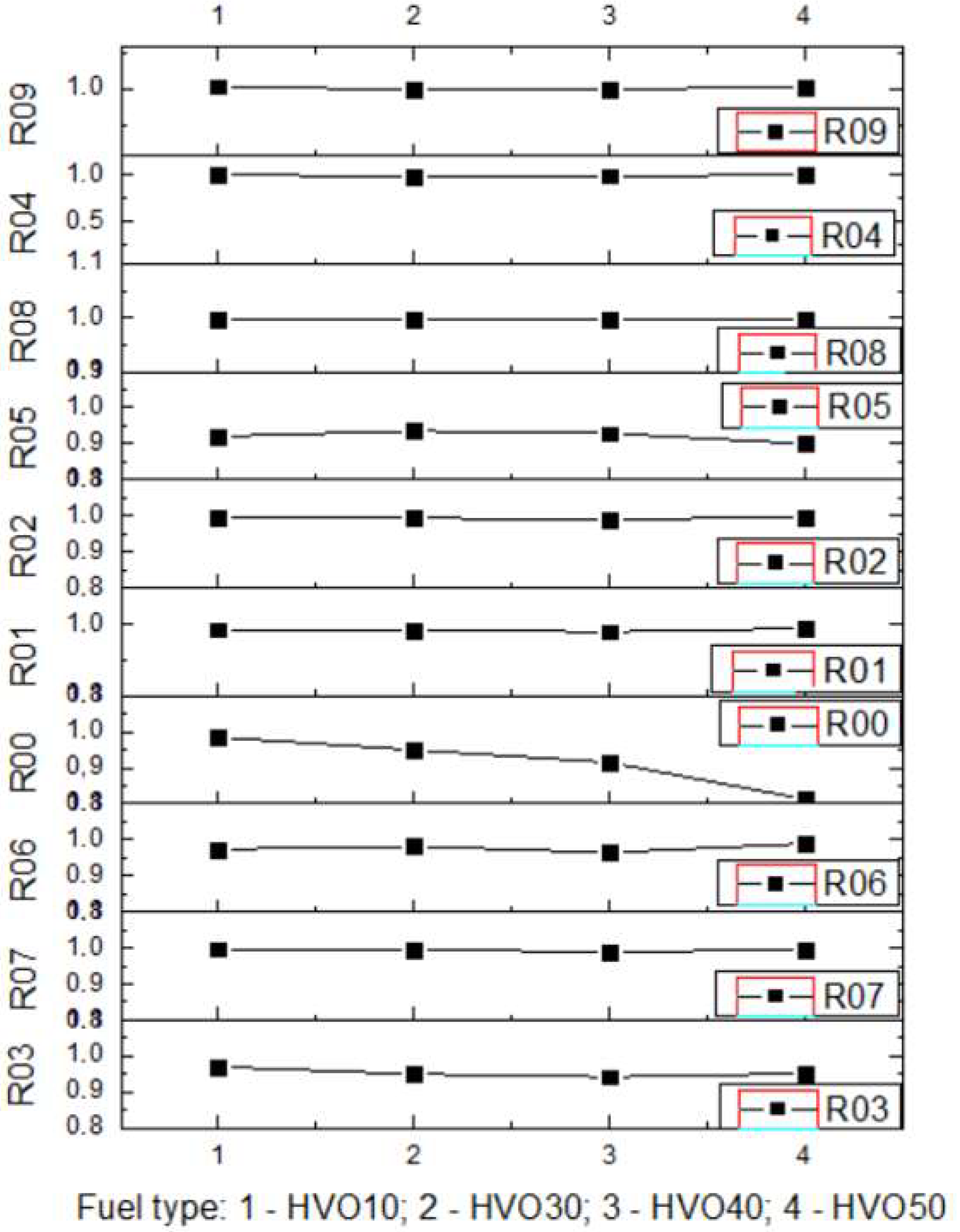
represent the impacts of parameters R01, R02, R07, R06, R08, R03, R05, R09, R04, and R00 on fuel type (HVO10, HVO30, HVO40, and HVO50). The nomenclature of the parameters is presented according to Table 4. All sets of parameters are presented in the following form, R01 … R10, for experimentally obtained values, and R01* … R10* for predicted values using ANN for validation of previously used experimental values in the regime of ANN training. A small deviation in the simulated values from the experimental values allows the work of ANN to be considered reliable.

BSFC depends on both the fuel properties and the engine operating mode. The lower heating value (LHV) of HVO100 is higher than that of D100, so, as the HVO concentration increases, the LHV of the fuel mixture increases (Table 3), and the BSFC decreases (Table 8). For all fuel blends, it is characteristic that the BSFC decreases as the load is increased from low to medium, or as the Start of Injection (SOI) is increased to the optimum. However, increasing the Exhaust Gas Recirculation (EGR) ratio shows an increasing trend of the BSFC. This means that the prediction of the BSFC depends on many factors, most of which we are trying to assess.

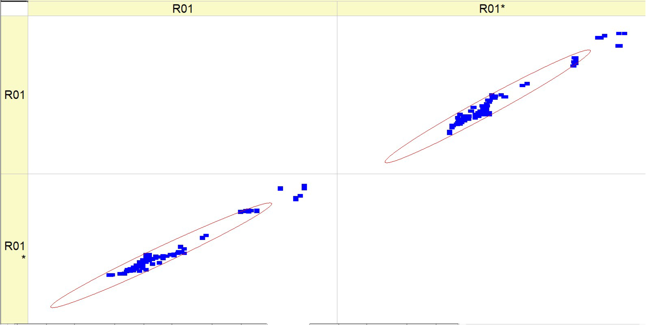
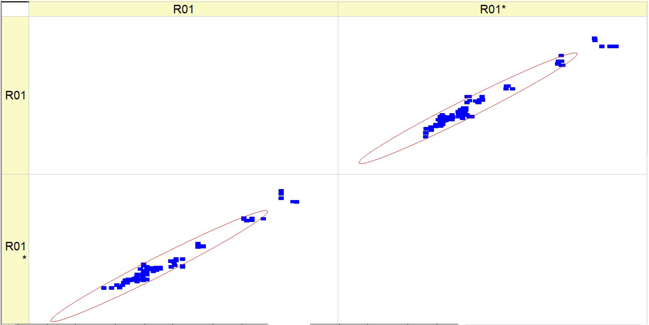
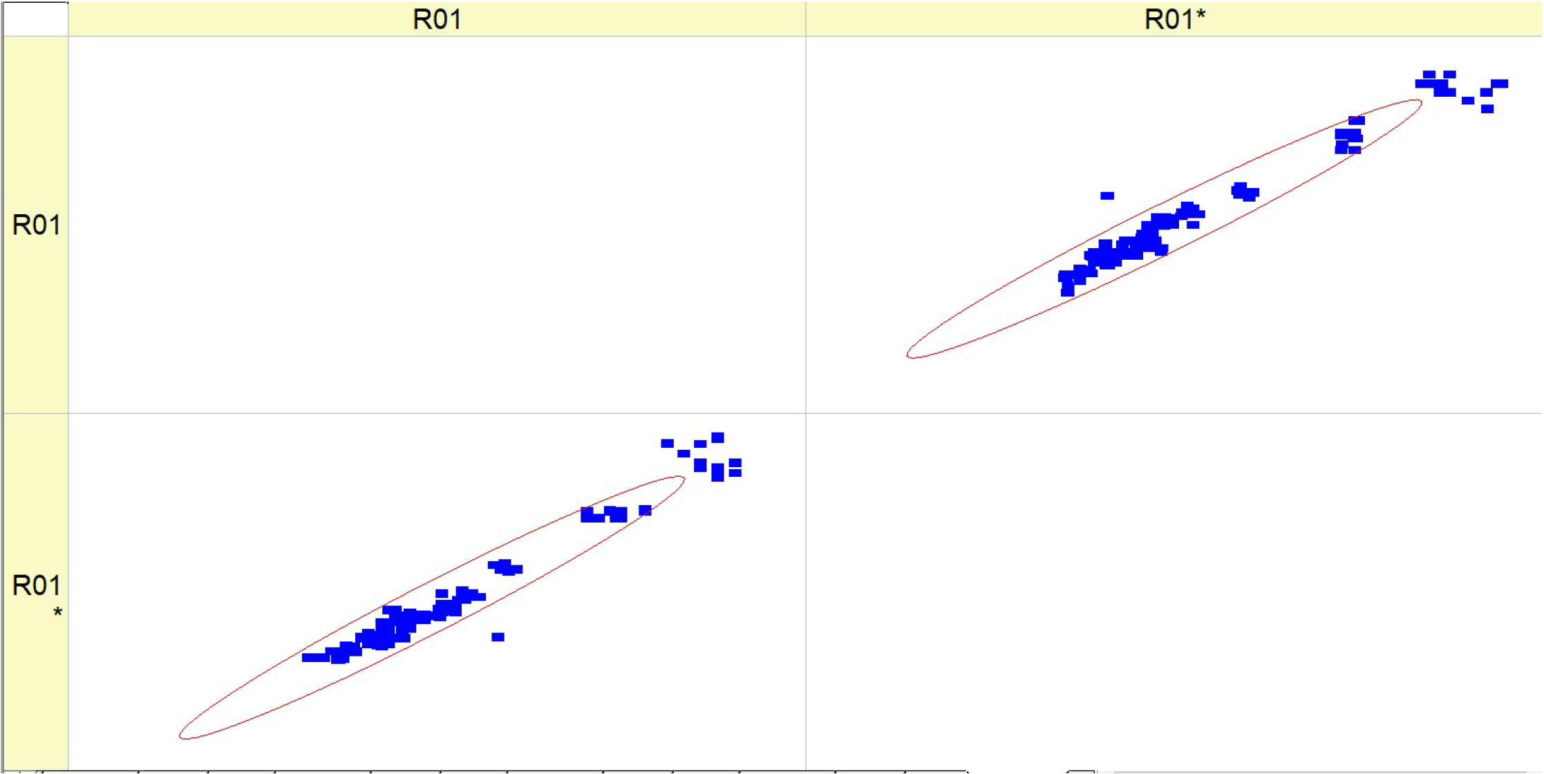
Table 8 (R01) displays histograms and scatter graphs representing various fuel types. The histograms display the distribution of BSFC readings over several runs, identified as RunNo. Each histogram provides a comparison between two datasets or situations, specifically referred to as R01 and R01*. The histograms for each fuel type exhibit distinct distribution patterns of BSFC, with some levels displaying smaller and taller peaks, while others exhibit broader distributions or several peaks. The scatter plots on the right show the relationship between anticipated BSFC values and actual measured values. An ideal forecast would result in all data points aligning perfectly along the diagonal line shown on the graph.

The clustering of data points along this diagonal line indicates the level of precision in the forecast. Scatter plots with points in close proximity to this line indicate more accuracy in the model’s predictions.

The histograms indicate that the distribution of BSFC values is influenced by the fuel type, which may be due to the varying impact of different fuel types on engine efficiency.

The scatter plots for each fuel type demonstrate the model’s proficiency in reliably predicting BSFC. A higher concentration of data points along the diagonal line would suggest a model with more reliability. It seems that the scatter plots for higher fuel types (HVO40 and HVO50) have data points that are tightly packed around the diagonal line, suggesting a better degree of accuracy in predicting outcomes at these levels.

The presence of R01 and R01* indicates that the parameter measurements are coherent, or that several models or methodologies are being compared under the same fuel type. Both the histograms and scatter plots suggest that the fuel type affects BSFC values and their prediction. Different fuel compositions may result in varying degrees of fuel efficiency and model accuracy.

To summarize, this chart compares the distribution of BSFC values at various fuel types with the accuracy of their forecasts. The variability in histograms and the concentration of scatter plot points indicate that both the real BSFC values and the model’s ability to forecast are affected by the fuel type used.

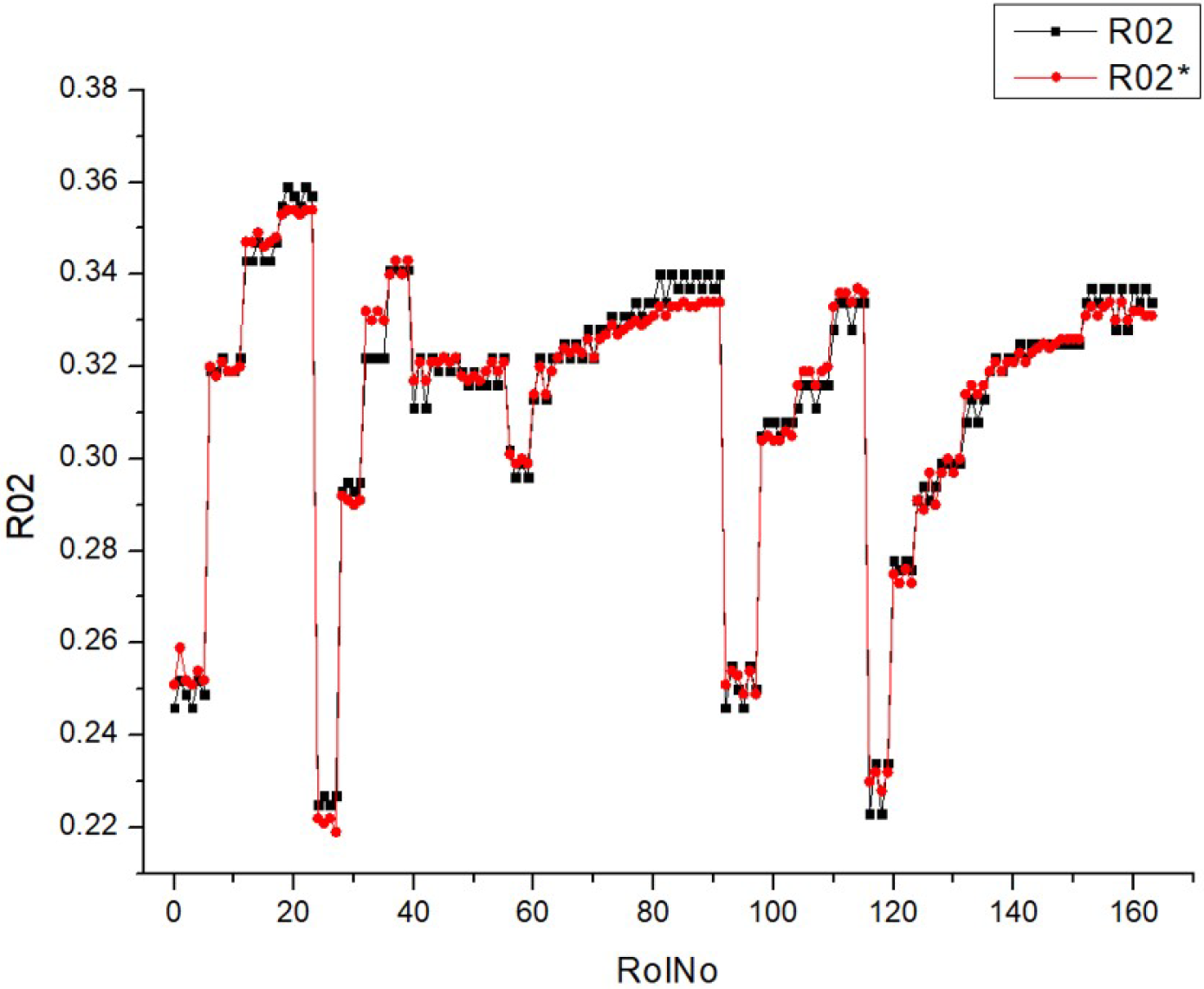
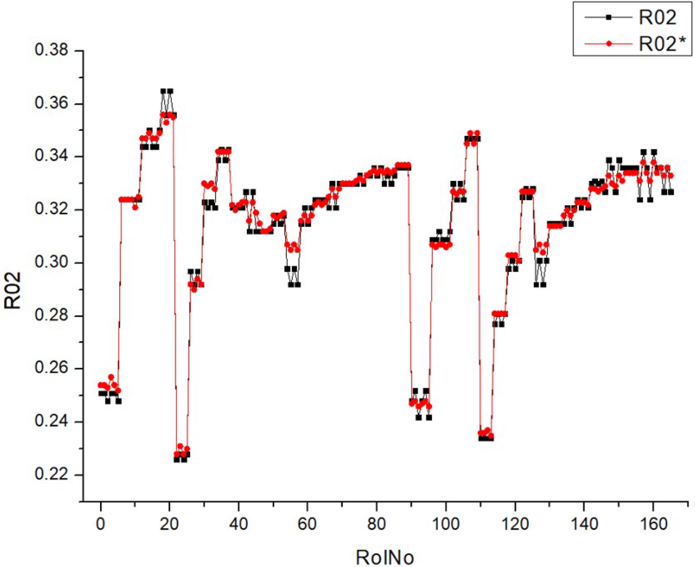
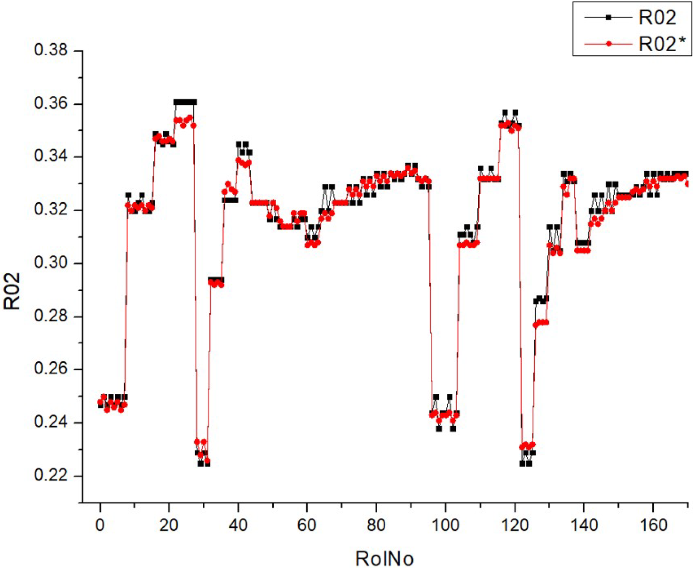
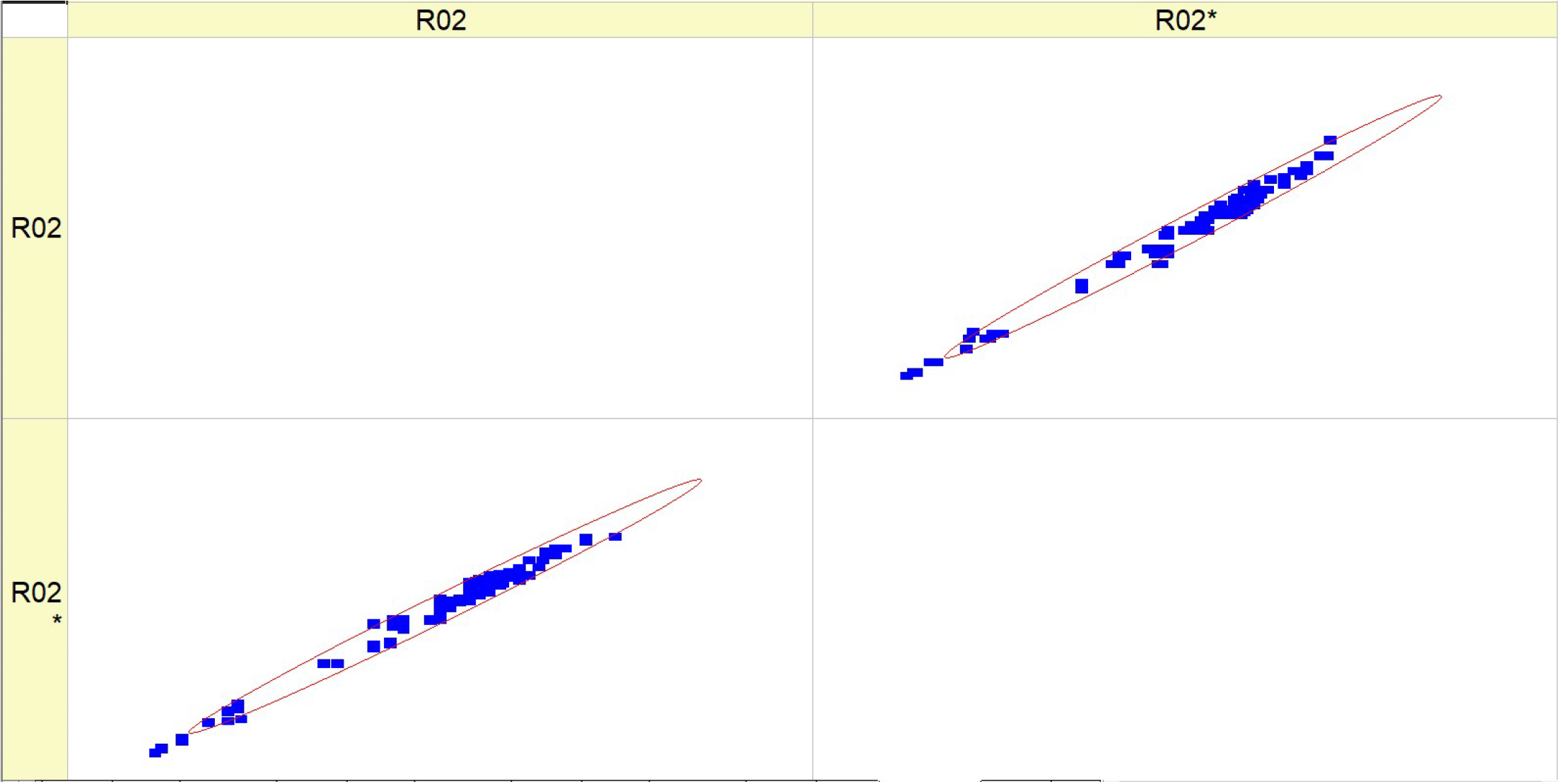
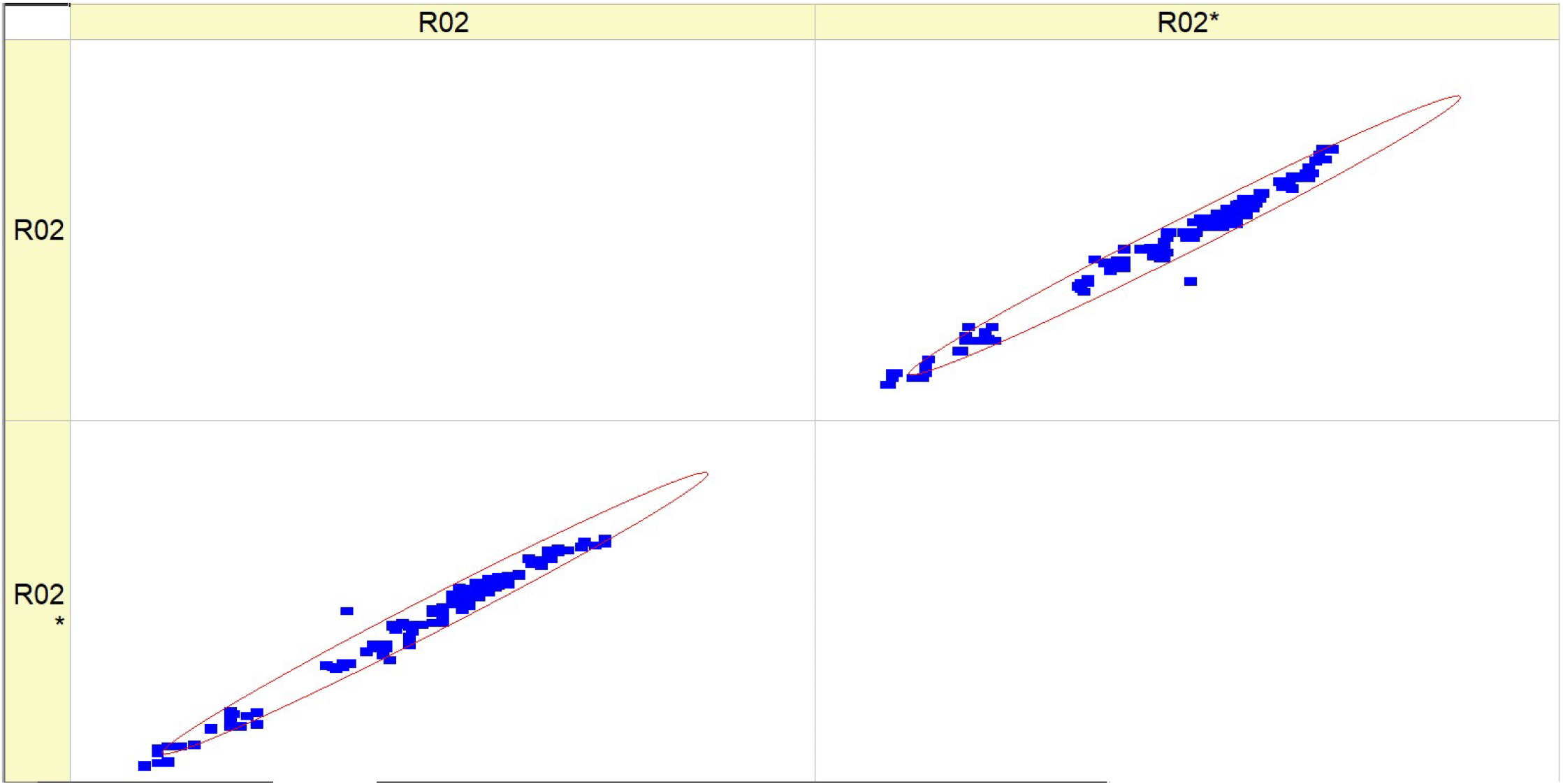
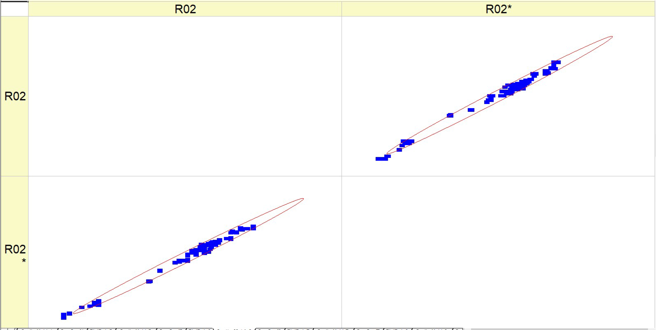
BTE shows the efficiency of the transformation of fuel energy (LHV) into the mechanical energy of the engine. The BTE depends on the BSFC and LHV of the fuel mixture. Table 9 (R02) displays a collection of histograms and scatter plots that pertain to different fuel types (HV010, HV030, HV040, and HV050).

Each histogram displays the frequency distribution of the BTE throughout a series of experiments, identified as RunNo. Two circumstances are shown for each fuel level, denoted as R02 and R02*, representing either distinct experiments or distinct measuring techniques. The histograms display the fluctuations in BTE for several runs, with particular levels demonstrating a higher frequency of certain efficiency ranges. The scatter plots on the right illustrate the comparison between the anticipated BTE values and the actual, measured values. Points that are closer to the diagonal line represent more precise forecasts. The dispersion of data points differs for each fuel type, with some fuels exhibiting a close grouping along the diagonal, indicating a high level of prediction precision.

The histograms depicting the fuel types demonstrate variations in the distribution and frequency of BTE readings. These findings indicate that the engine’s efficiency fluctuates not just across different runs but also in accordance with the specific kind of fuel used.

The scatter plots indicate that the accuracy of the prediction model fluctuates depending on the fuel types. This is demonstrated by the closeness of data points to the diagonal line, where tighter clusters indicate more precise forecasts. There is a noticeable pattern where fuel types HV040 and HV050 contain data points that are closely clustered around the diagonal line, suggesting that there may be increased accuracy in predictions at these levels. The existence of two separate sets of outcomes for each fuel type (R02 and R02*) indicates that the behavior of the parameter is constant across several experiments or that the model’s forecasts can be replicated under different circumstances. Both of the histograms and scatter plots suggest a correlation between fuel kinds and their efficiencies, where the BTE is impacted by the specific properties of each fuel type. This, in turn, impacts the accuracy of the model’s predictions.

To summarize, the image presents a comparison between the actual and expected BTE of engines that use varying volumes of fuel. The discrepancies in the histograms and the concentration of data points in the scatter plots along the diagonal line suggest that the performance of the engine and the predictive capability of the model are affected by the kind of fuel used.

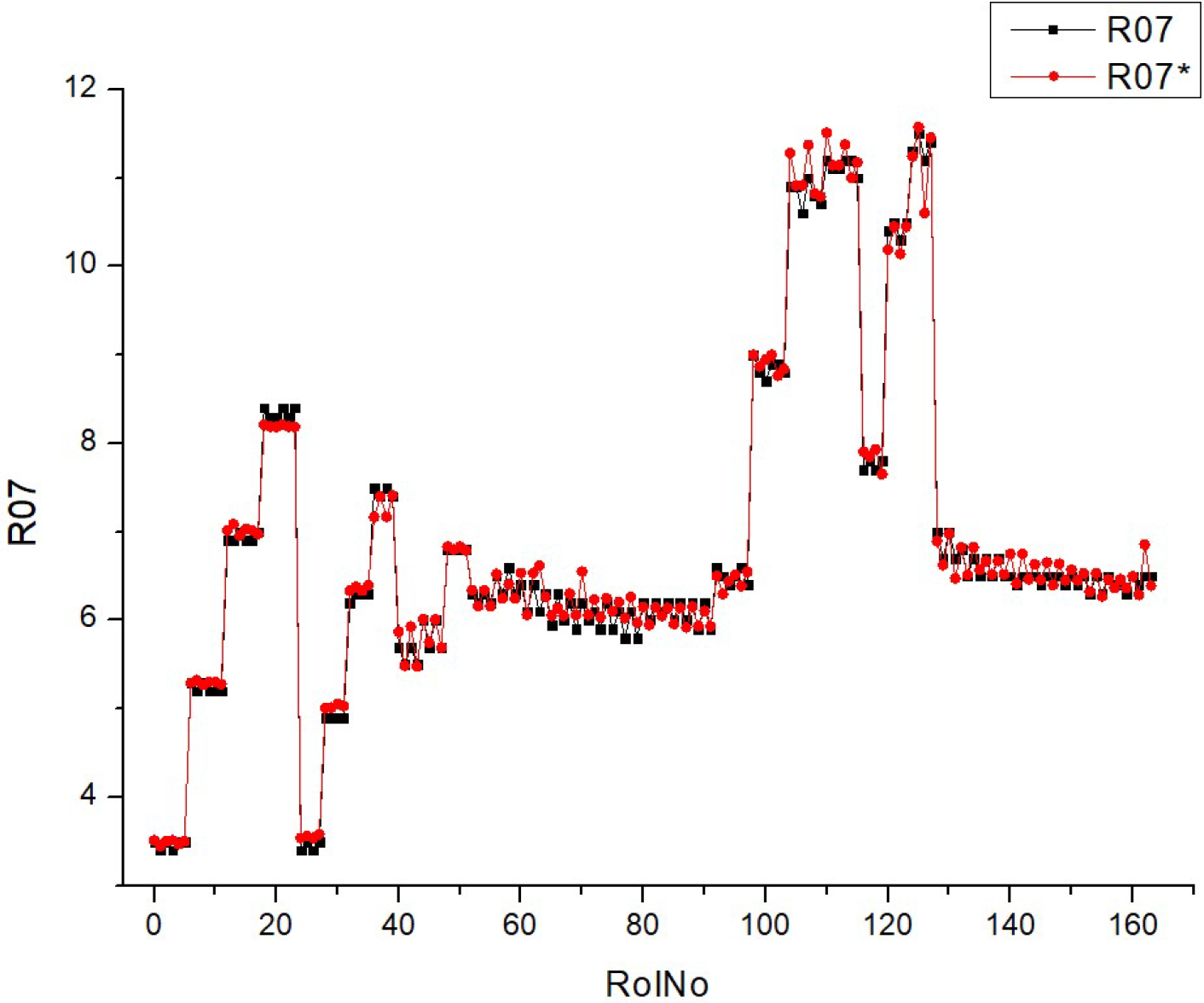
The concentration of CO₂ in the exhaust gases depends mainly on fuel consumption, fuel composition (C/H ratio), completeness of the combustion process, and the excess air ratio in the cylinder. As the engine load is increased, the CO₂ concentration rises by a significant amount, but as the share of HVO in the fuel mixture is increased, the CO₂ concentration is lower (Table 10) due to the lower C/H ratio and the lower BSFC. Higher EGR leads to a significant increase in CO₂ concentrations by reducing excess air, but optimizing the SOI leads to a slight reduction in CO₂ concentrations due to reduced fuel consumption.

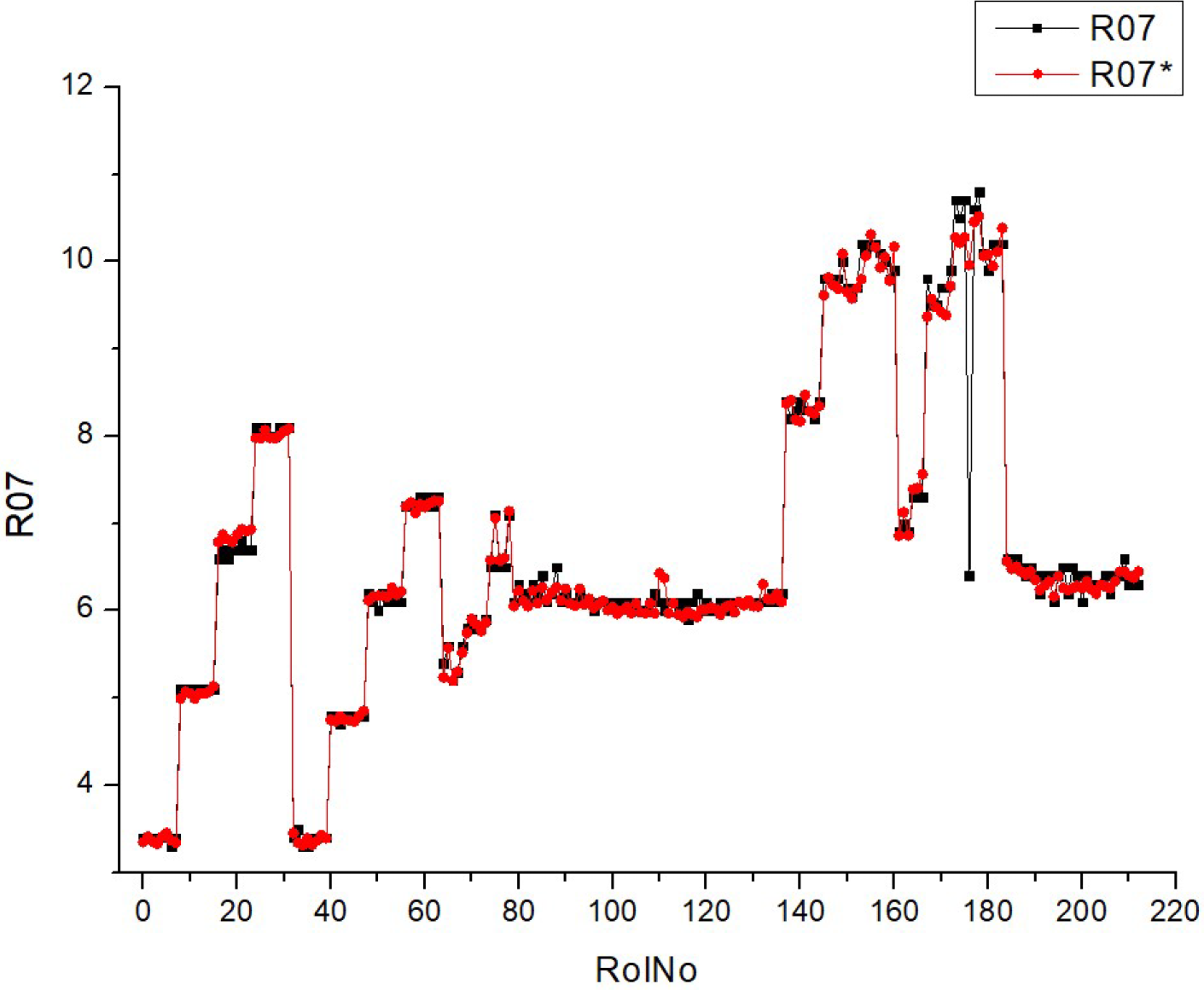
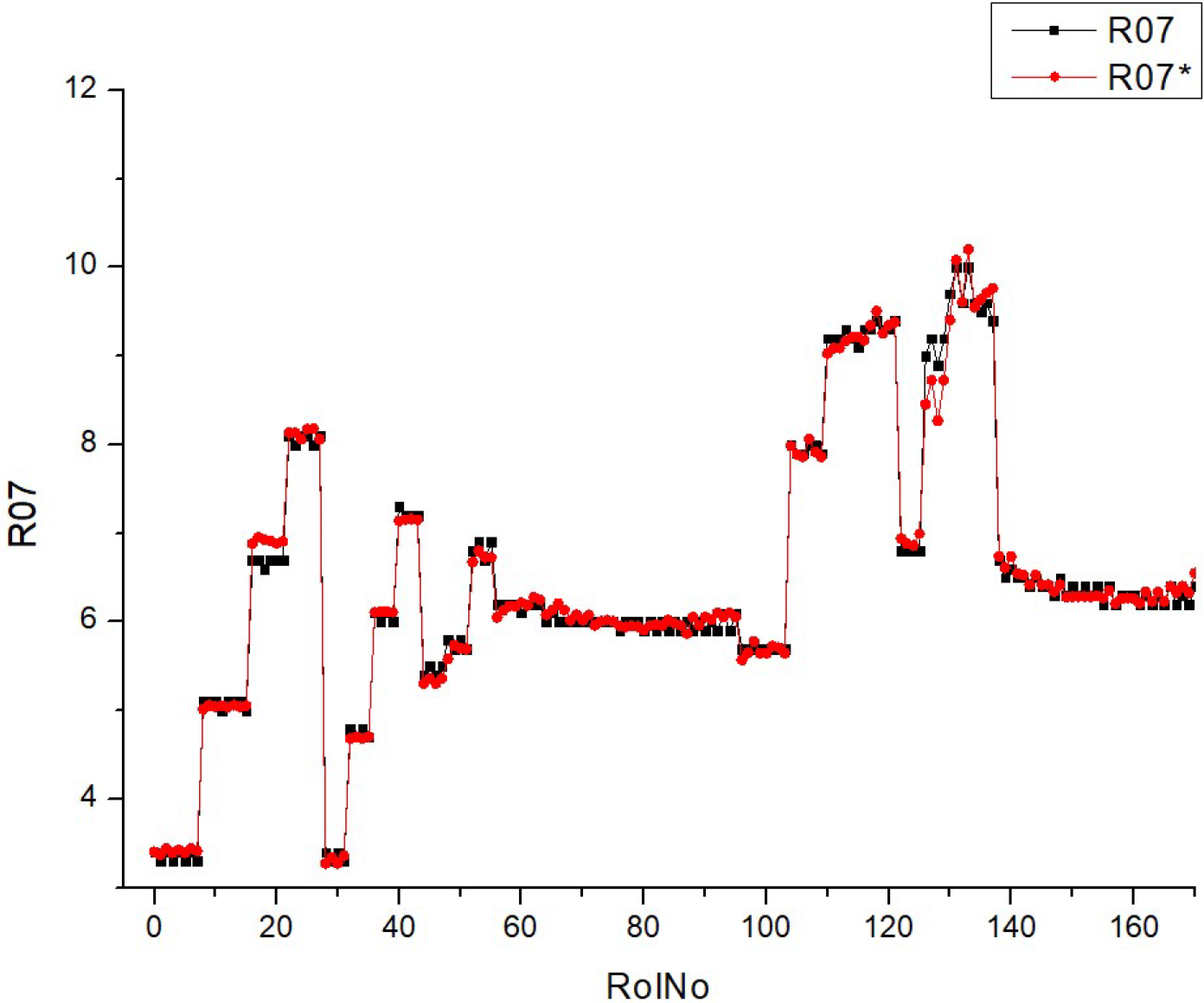
Table 10 (R07) displays a collection of histograms and scatter plots that pertain to either CO₂ concentration. The histograms illustrate the distribution of a certain parameter over numerous runs (RunNo). The unspecified parameter is presumably associated with emissions or another fuel attribute at varying concentrations of CO₂.

Each graphic has two superimposed histograms, labeled R07 and R07*, which likely reflect distinct datasets. The histograms exhibit different shapes and distributions for each fuel type, suggesting that the parameter is sensitive to variations in the CO₂ content of the fuel. The presence of peaks in the histograms indicates that certain values of the parameter occur more often, while the width of the peaks reflects the extent of fluctuation around these common values.

The scatter plots visually depict the correlation between expected and actual values of a parameter, where the dots are distributed around a diagonal line that represents the ideal prediction. The closeness of the dots to the diagonal line indicates the precision of the forecasts. Greater proximity between data points indicates higher levels of prediction precision. The scatter plots demonstrate a constant increase in predicted accuracy throughout various fuel types, as demonstrated by the concentration of data points along the diagonal line. This indicates that the model’s predictions are in good agreement with the actual results, particularly when the fuel types are greater.

When comparing histograms and scatter plots, we may detect a correlation between the concentration and spread of fuel types in histograms (which indicates the amount of variation in the parameter) and the clustering of scatter plot points around the diagonal line (which indicates the accuracy of forecasts). The findings for R07 and R07* in both histograms and scatter plots exhibit comparable patterns, suggesting that the observed correlations are stable across other datasets or situations.

The predictability of the parameter increases when the fuel types rise from HV010 to HV050. This improvement might be due to changes in CO₂ concentration or other relevant aspects.

Essentially, this picture depicts the correlation between fuel types and a certain parameter associated with CO₂, as well as the accuracy of a predictive algorithm in forecasting this parameter. The repeatability of the data between R07 and R07* is shown by the resemblance in the distributions and trends seen in the scatter plot.

The comparison is made across multiple fuel types (HVO10, HVO30, HVO40, and HVO50) for Table R07. The morphology and dispersion of the histograms indicate that the distribution of the observed parameter fluctuates across different fuel types. Some histograms have more pronounced peaks, indicating a higher frequency of certain values, while others display a wider distribution, suggesting more variability. The quantity and positions of the peaks vary, indicating that the parameter reacts distinctively to changes in fuel blends.

The scatter plots illustrate that the clustering of data points around the diagonal line, which represents the accuracy of predictions, differs depending on the fuel type. Certain fuel types may exhibit a higher degree of data point clustering, indicating a greater level of accuracy in predictions. The dispersion seen in the scatter plots, deviating from the ideal diagonal line of perfect prediction, suggests that the model’s predictive ability varies among various fuel types. This may indicate variations in the predictability of the parameter based on the fuel mixture. The scatter plots exhibit a discernible pattern where an increase in fuel type corresponds to improved prediction accuracy, demonstrated by the data points grouping in closer proximity to the diagonal line.

Although there may be variations in the details, the histograms generally exhibit a multimodal distribution for each fuel type, suggesting that the parameter has numerous prevalent values or states that it alternates between. The inclusion of two histograms in each plot (R07 and R07*) indicates the existence of consistent patterns of behavior for the parameter across many datasets or experimental settings.

To summarize, the fuels listed in Table R07 have distinct features in their histograms and differ in the accuracy of their predictions, as shown in the scatter plots. However, they also have similarities in terms of the overall patterns of prediction enhancement with increased fuel types and the shapes of their data distributions. These similarities and differences may provide valuable information about how the composition of fuel affects the parameter being measured and the accuracy of the model used for making predictions.

The specific exhaust emissions of individual components give a more objective picture of the emissions of each component. In this case, the mass of pollutants per unit of engine power (g/kWh) is calculated. In this way, the specific CO₂ emissions (SCO₂) also show the positive impact of HVO on reducing these greenhouse gases (Table 10). But, unlike CO₂ concentration, SCO₂ emission decreases with increasing engine load, and it can be significantly reduced by adjusting the SOI.

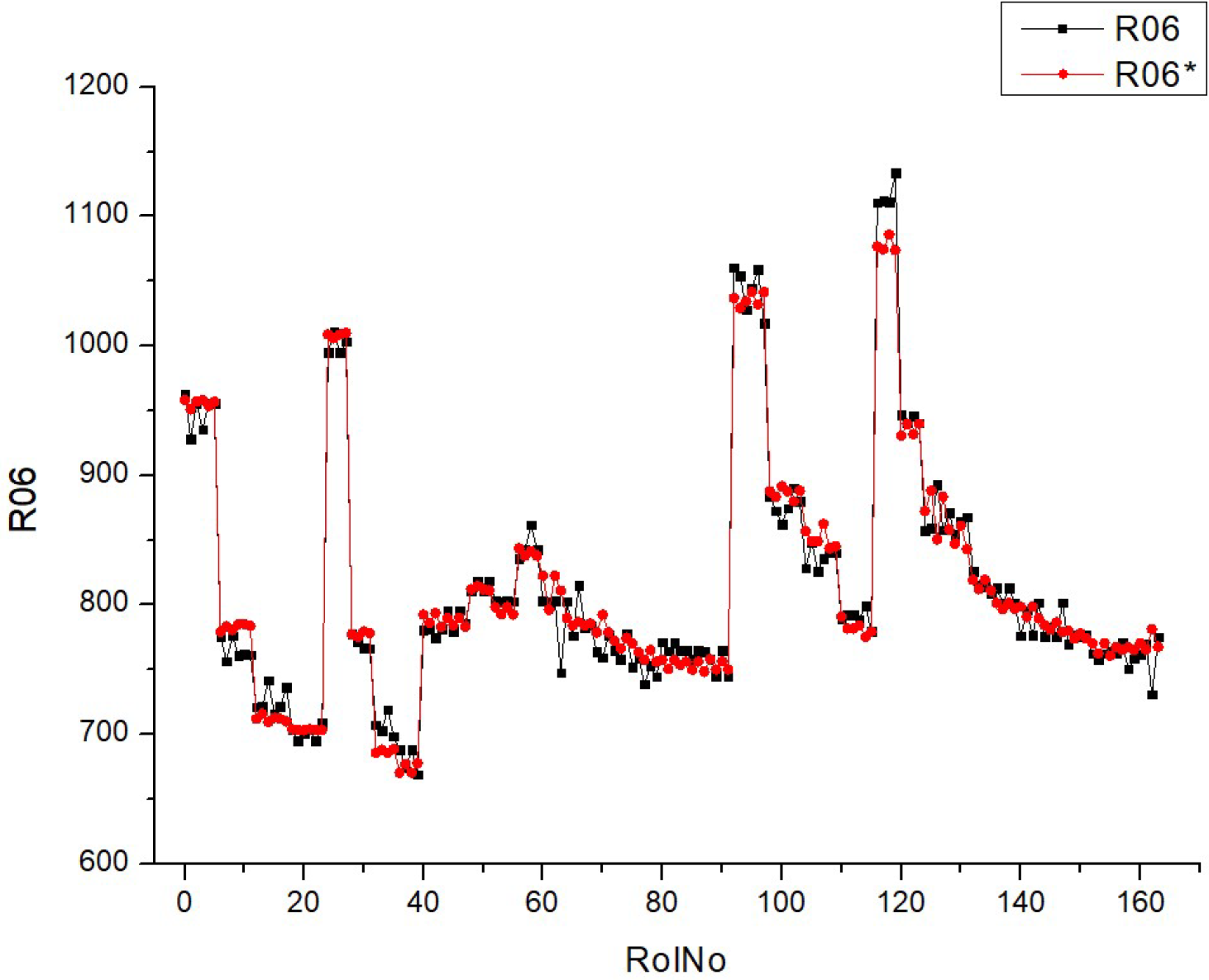
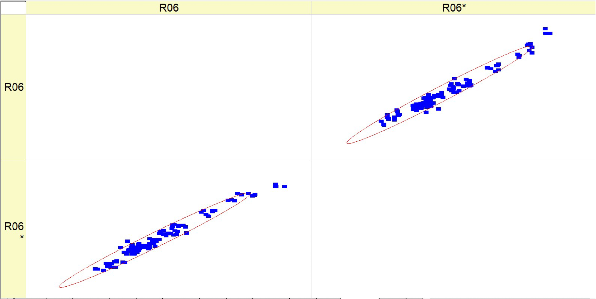
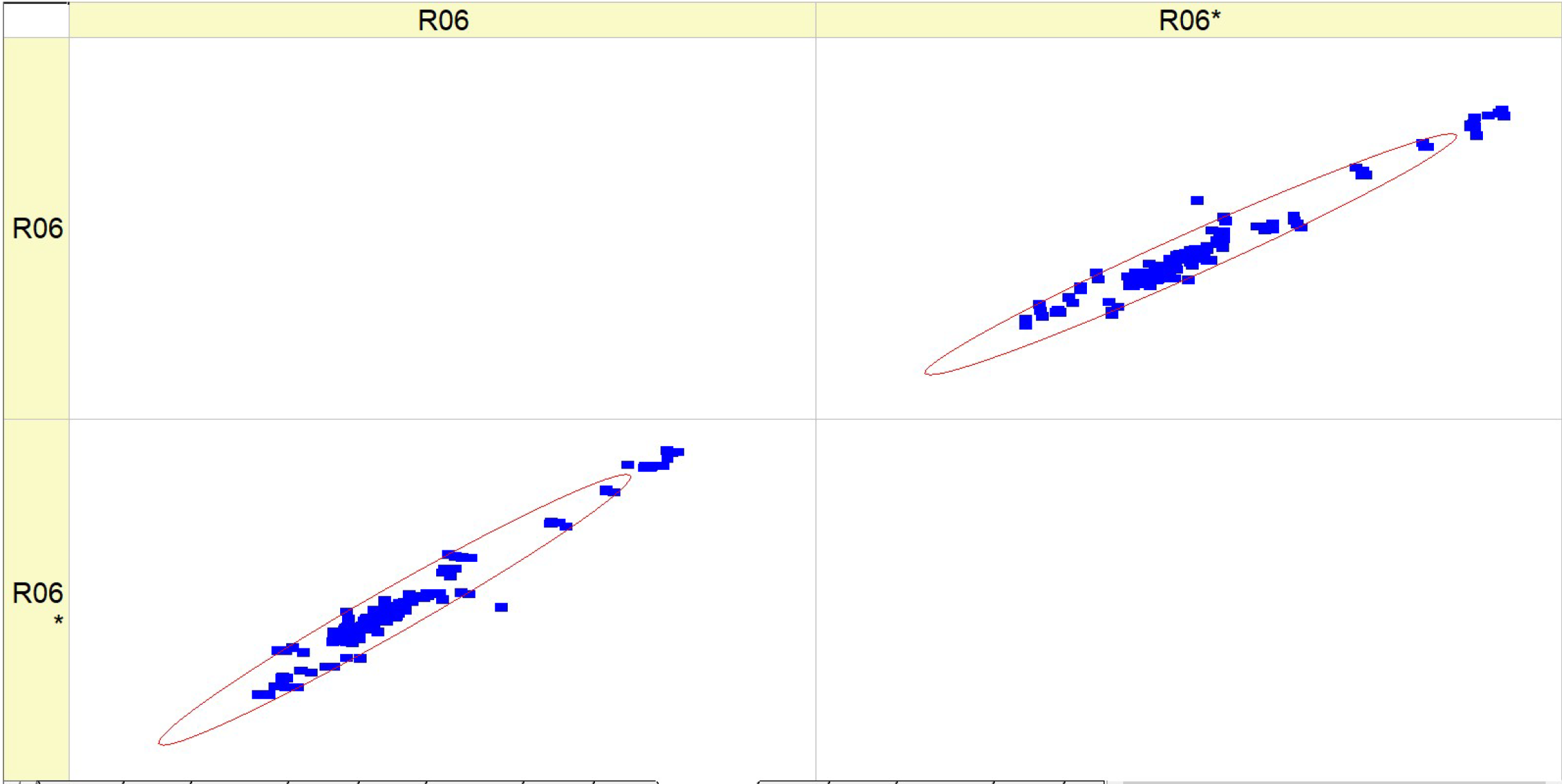
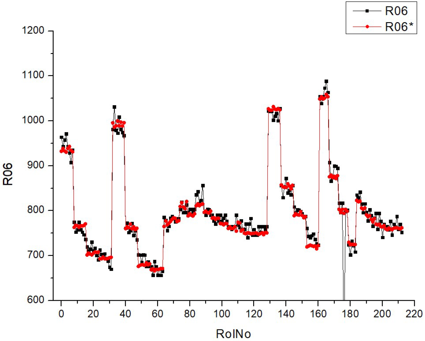
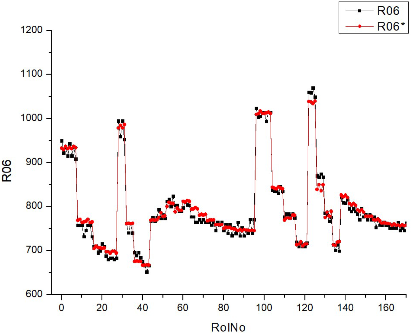
Table 11 (R06) includes a collection of histograms and scatter plots that are related to the SCO₂ result. Typically, there is an observed correlation between histograms with narrower peaks and scatter plots with data points that are more densely clustered around the diagonal. Consequently, when there is a decrease in the variability of the parameter being monitored, the predictions become more precise.

The consistency between the histograms and scatter plots for both R06 and R06* indicates that the observed associations are dependable and that the model’s prediction ability remains constant under varying situations. There is an implicit assumption that increasing the fuel types leads to greater stability and predictability of the parameter associated with SCO₂.

Table 11 presumably demonstrates the impact of various fuel compositions on a particular parameter linked to supercritical SCO₂, as well as the predictive model’s ability to effectively anticipate this parameter. The performance of the model shows enhancement with increased fuel types, as demonstrated by the concentration of data points around the diagonal on the scatter plots. The validation of the study’s conclusions relies heavily on the repeatability of results, as shown by the parallels seen between R06 and R06*.

The distribution of data inside the histograms changes depending on the fuel types. Certain histograms have a broader distribution, while others have tighter peaks, suggesting varying levels of concentration of the parameter values. The quantity and acuteness of peaks vary across the fuel types, indicating potential flexibility in the parameter’s response to different fuel compositions. The scatter plots exhibit varying degrees of conformity to the diagonal line, indicating differences in the prediction precision of the model for each fuel type. For some types of fuels, the data points are closely grouped around the diagonal, which suggests a greater level of accuracy in predictions. In contrast, for other fuels, the data points are more spread out. The scatter plots may exhibit varying deviations from the diagonal line, indicating that the model’s ability to make accurate predictions depending on fuel mix may vary. The scatter plots provide a clear pattern of progress in fuel type prediction, as demonstrated by the growing concentration of data points along the diagonal line. This indicates a steady trend in which the model’s forecasts are enhanced as the fuel percentages increase. The histograms for all fuel types have a multimodal pattern, indicating that the parameter has many common values or behaviors over the range of runs.

The histograms for conditions R06 and R06* exhibit comparable distribution shapes within each fuel type, suggesting that the model’s performance is stable across many datasets or trials. Essentially, the fuels included in Table R06 exhibit distinct characteristics in terms of parameter distribution and prediction accuracy. However, they also have a commonality in terms of the overall improving trend in model predictions and the form of their distributions. The presence of a multimodal distribution suggests that the parameter behaves consistently across various fuel compositions. Additionally, the improved accuracy of forecasts at higher fuel types indicates a potential link between fuel composition and the predictability of the parameter.

Analyzing the histograms and scatter plots of Tables R06 and R07 allows for the identification of any disparities or similarities in the parameter distribution and the precision of projected values. Upon first observation, the morphologies of the distributions in R06 and R07 have some resemblance, as they both display many peaks (modes) across the runs.

An observable distinction may be seen in the extent and elevation of the summits. R07 has a greater number of well-defined peaks with less overlap between the two conditions (R07 and R07*) in comparison to R06. This observation suggests a more consistent and unique behavior of the parameter across several experimental circumstances.

The scatter plots for R06 and R07 depict the correlation between the anticipated and observed values of the parameter under investigation.

Both R06 and R07 provide scatter plots that show an increase in forecast precision as the fuel type rises (with points closer to the diagonal line). Nevertheless, the plots obtained from R07 exhibit a more compact clustering pattern along the diagonal, particularly at higher fuel types, implying superior predictive accuracy in R07 compared to R06.

The extent of dispersion, or how far off the points are distributed from the diagonal line, also provides insight into the variability of the forecast. Although both R06 and R07 exhibit scatter, the plots in R07 may suggest little reduced variance, implying a more precise prediction model in R07.

Upon examining both the histograms and the scatter plots together, it seems that the R07 model has a slightly higher level of refinement or tuning. This is evident from the presence of more pronounced peaks in the histograms and a more compact clustering in the scatter plots.

It is worth mentioning that there is a constant improvement in the accuracy of forecasts as fuel types grow in both R06 and R07. This indicates that the model’s predictions become more dependable with larger concentrations of the parameter being researched.

The comparison between R06 and R07 reveals parallels in terms of the general patterns, indicating enhanced forecasts at greater fuel types. Nevertheless, R07 may have somewhat more accurate distributions of the parameter and enhanced precision in predictions, as shown by more compact clusters along the diagonal in the scatter plots and more distinct peaks in the histograms. These findings, however, are presented with the proviso that the comparisons are only based on the visual evaluation of the figures supplied, as there is no access to the actual data or extra context from the research.

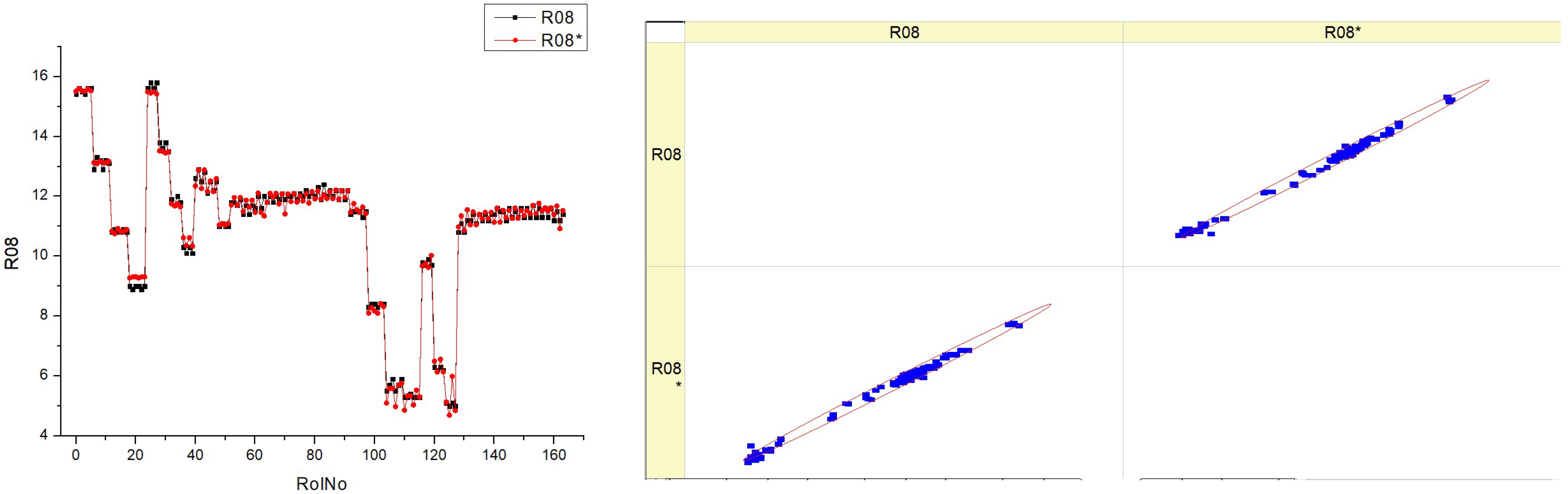
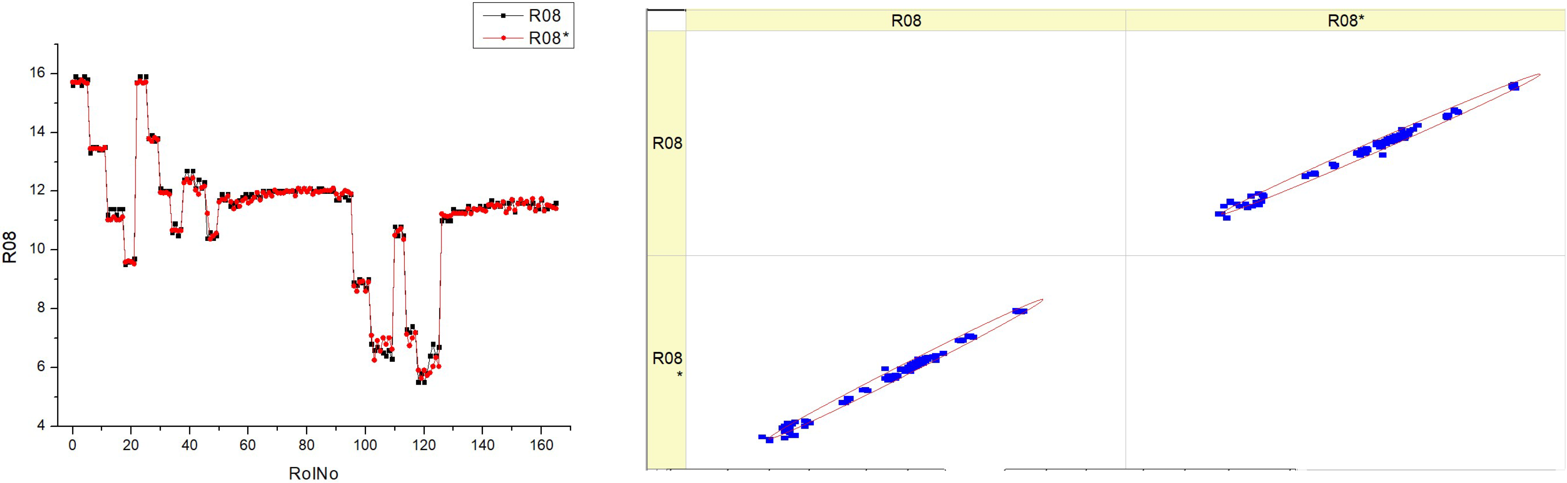
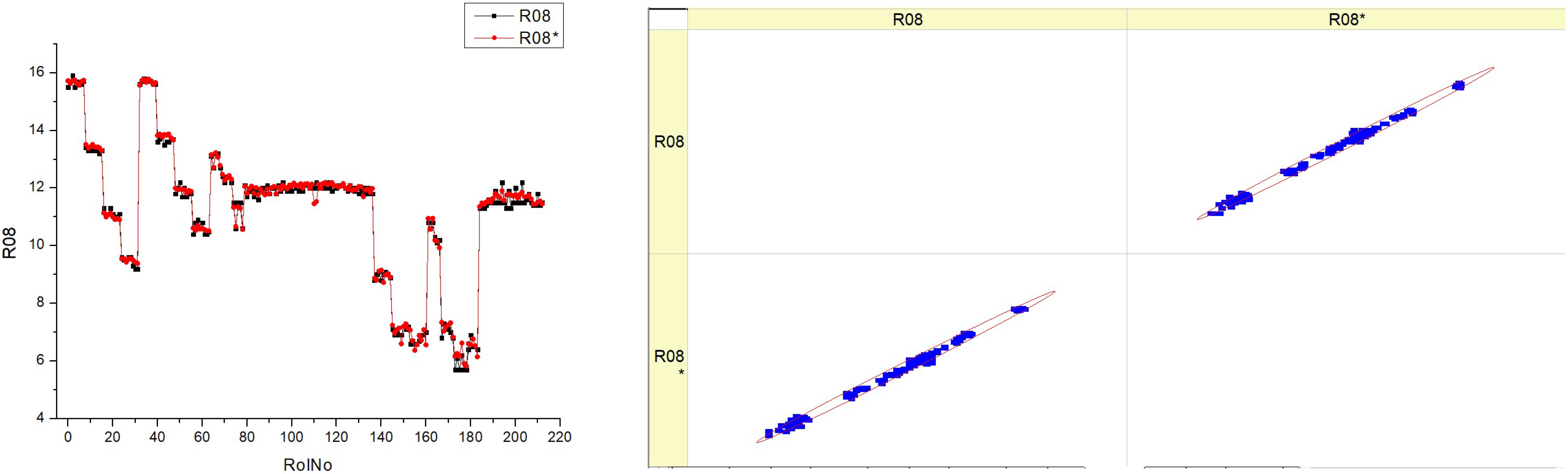
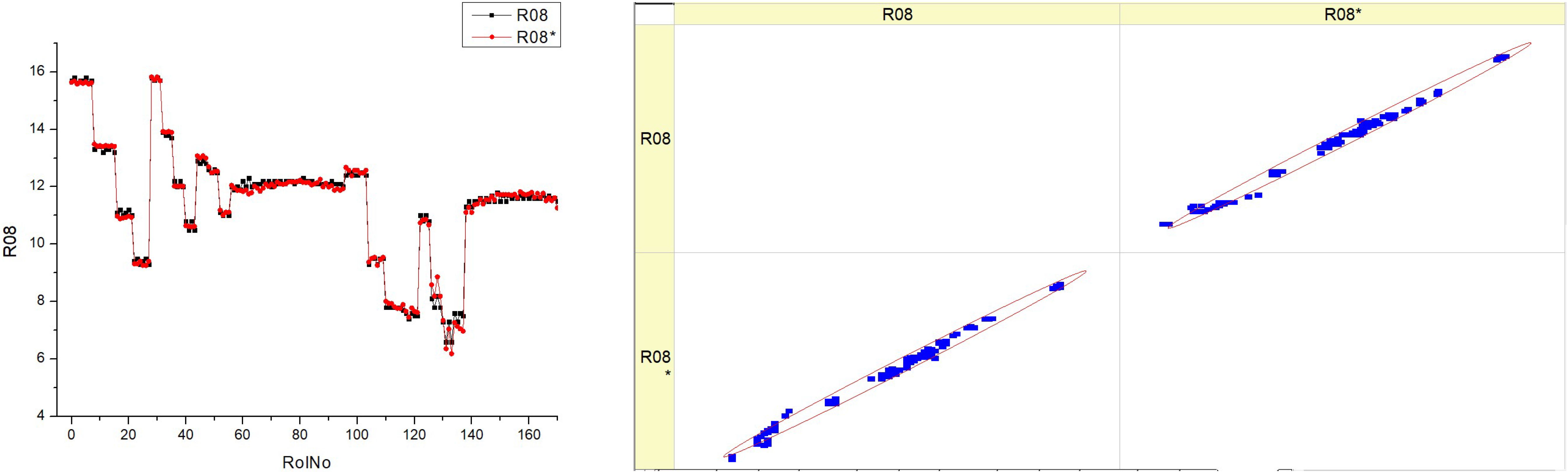
The concentration of O₂ in the exhaust provides additional information about the combustion conditions in the cylinder of the engine. A lower O₂ concentration indicates that the fuel has less excess air and is less likely to fully oxidize. This trend is characterized by an increase in the EGR ratio (Table 12) and confirmed by an increase in smokiness. An increase in the concentration of HVO in the fuel mixture has no significant effect on the O₂ concentration in the exhaust gas, as the higher air requirement for HVO combustion (Table 3) is compensated by the lower HVO consumption.

Table 12 (R08) seems to display measurements and an analysis of O₂ concentration in exhaust gases. The histograms on the left show the distribution of the O₂% for each fuel type in several runs, denoted as RunNo. Each fuel type is represented by two datasets, labeled R08 and R08*, which may indicate distinct experimental circumstances.

The histograms illustrate the variability in the oxygen content at different fuel types. Some histograms show a high occurrence of certain oxygen values, while others exhibit a broader range of values throughout the experiments.

The scatter plots on the right show the correlation between the anticipated values of O₂% and the actual measured values. The proximity of the data points to the diagonal line directly correlates with the accuracy of the forecasts.

The graphs exhibit variations based on the fuel type, with some plots displaying data points closely grouped around the diagonal line, suggesting a greater degree of accuracy in predictions. The histograms demonstrate that the O₂ distribution varies depending on the fuel type, indicating that various fuel types may have distinct effects on the combustion process. The scatter plots illustrate the accuracy of the predictive algorithm in forecasting the O₂%. The proximity of the dots to the diagonal line differs across different fuel types, suggesting that the accuracy of the model may be affected by the precise composition of the fuel.

There could be a pattern where fuel types HV040 and HV050 show scatter plots with data points clustered more closely around the diagonal line. This might indicate that the model’s predictions are more precise for these specific fuel types.

The existence of two data series for each fuel type (R08 and R08*) suggests the potential for reliable measurement across many trials or situations, or the strength of the prediction model used.

The combination of histograms and scatter plots may provide insights into the impact of various fuel types on the oxygen content in exhaust gases, as well as the predictive capability of a model in relation to this content.

Essentially, the diagram illustrates the comparison between the observed and forecasted levels of oxygen content at various fuel types. It demonstrates the variations in both the measured percentage of O₂ in real-world scenarios and the expected values, depending on the kind of fuel used. The discrepancies in histograms and the aggregation of data points in scatter plots suggest a correlation between fuel composition and combustion efficiency, as shown by the oxygen concentration in the exhaust gases.

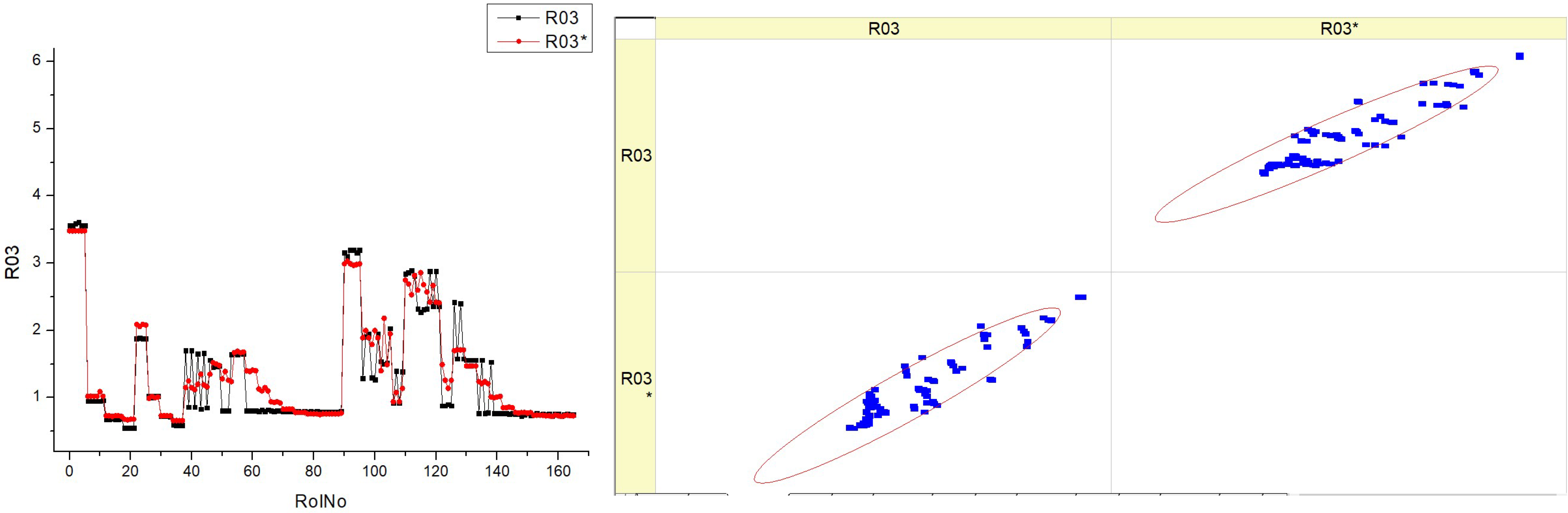
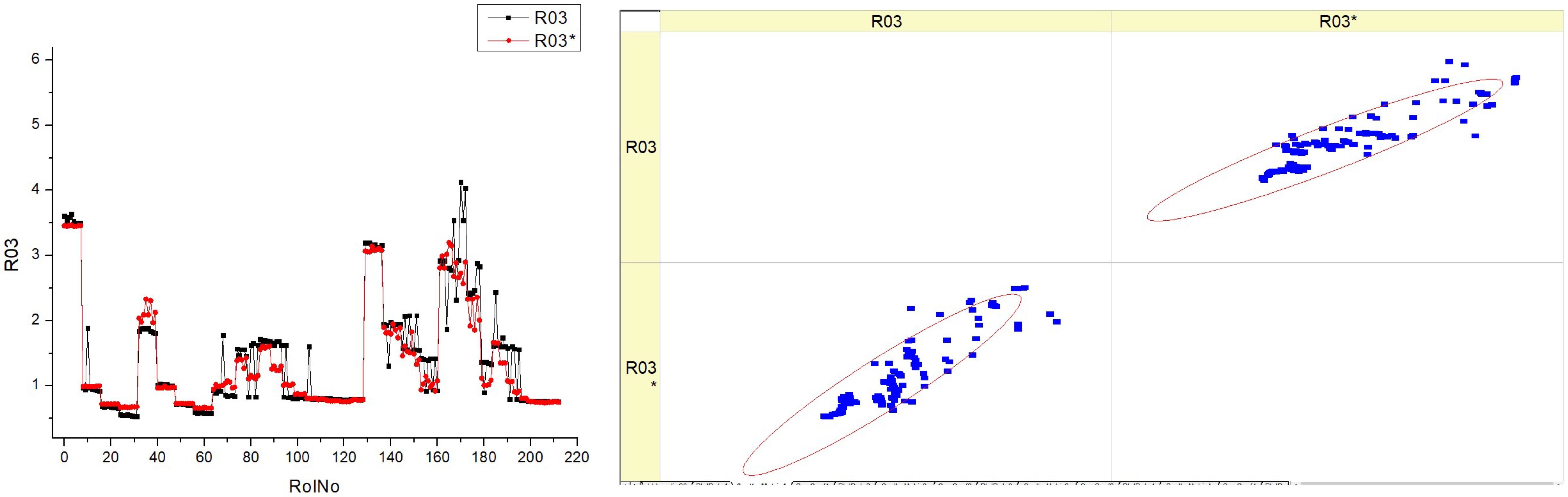
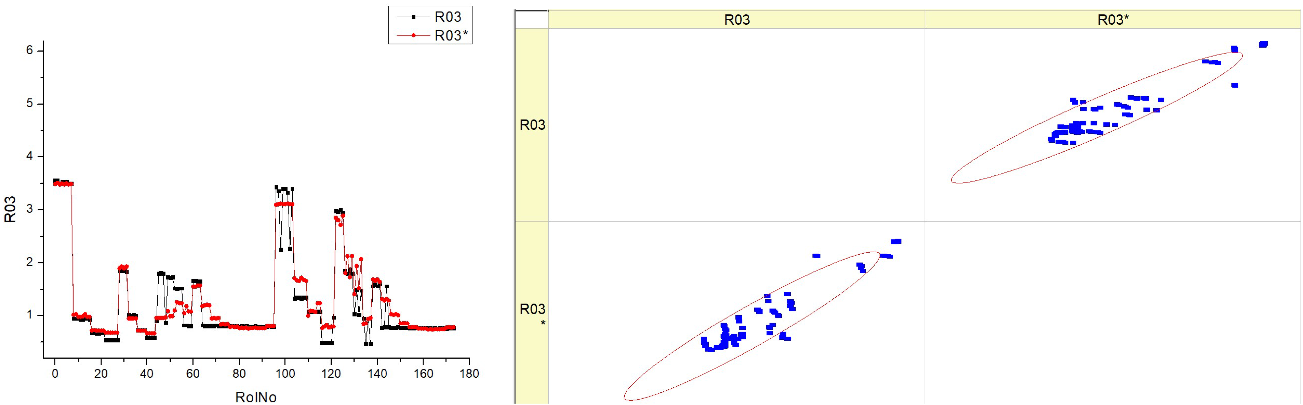
CO and HC in the exhaust indicate incomplete combustion. This trend is typical when the engine load is constant, and increasing the EGR ratio decreases the O₂ concentration due to the recirculation of combustion products (CO₂ and H₂O) into the cylinder. However, as the engine load increases, specific carbon monoxide emissions (SCO) decrease (Table 13), as the concentration of CO increases less compared to how much the load increases. Increasing the concentration of HVO in the fuel mixture shows a decreasing trend in SCO emissions due to the decreasing C/H ratio of the fuel and better HVO atomization and combustion characteristics. It is likely that the prediction accuracy for SCO is lower compared to the other parameters analyzed, as the CO concentration in the compression ignition engine is close to the minimum measurement limit of the gas analyzer.

There are four distinct datasets (R03), labeled HVO10, HVO30, HVO40, and HVO50, each representing a different fuel type (Table 13). Each dataset consists of two types of graphical representations: a histogram and a scatter plot. Each graphic has two superimposed histograms, which presumably reflect two distinct situations or datasets (R03 and R03*) for the sake of comparison. The histograms display fluctuations in the parameter throughout several runs, with some runs demonstrating a greater occurrence of certain parameter values. The histograms exhibit varying shapes and distributions for different fuel levels, indicating that the parameter being monitored is responsive to changes in the fuel type. The scatter plots seem to be a visual representation that compares the anticipated values with the actual values of a certain parameter. This comparison is represented by the presence of linear trend lines. Every data point on the scatter plot corresponds to a specific measurement, and its position on the plot indicates its actual value compared to its expected value.

In an ideal scenario, if forecasts are flawless, all data points would align precisely along the diagonal line. Any deviations from this line indicate flaws in prediction. The scatter plots indicate that when the fuel type rises (from HVO10 to HVO50), the data points tend to form tighter clusters around the diagonal line. This suggests that the prediction model gets more precise and reliable at higher fuel types.

The figure does not clearly demonstrate the direct link between the histograms and the scatter plots. However, it suggests that as the parameter’s variability lowers (resulting in a narrower histogram), the accuracy of the predictions improves (evidenced by scatter points closer to the diagonal).

It seems that increasing the fuel types (HVO30 to HVO50) leads to more consistent outcomes, as demonstrated by the closer grouping of peaks in the histogram and points in the scatter plot.

The appearance of two histograms on each plot (R03 and R03*) suggests the possibility of two distinct trials or studies, each exhibiting slightly different distributions. This indicates the repeatability or variability of the findings under slightly varied circumstances.

Essentially, this picture is probably illustrating how the amount of fuel affects the stability of a certain parameter and the precision of its forecast. Additionally, it assesses the outcomes of two datasets or situations in order to determine their consistency or emphasize disparities between them.

Now, let us analyze the distinctions and resemblances among these fuels. The peaks and spread of the histogram vary across various fuel types. This indicates that the parameter being measured has distinct distributions for each fuel type. The peaks exhibit variations in both height and sharpness, suggesting that some fuels possess a higher concentration of certain parameter values, while others have a broader range. For instance, HVO10 may have a smaller peak in comparison to HVO30, indicating a higher level of consistency in its behavior at a certain run number. The distribution of points along the diagonal line varies across the different fuels. A tighter cluster of points in one fuel type implies more accuracy in the model’s predictions for that particular fuel compared to others.

The scatter plots show that the distance of the points from the diagonal line, which represents perfect prediction, may vary for each fuel type. This indicates that the model’s ability to forecast the parameter changes depending on the fuel composition.

Both the histograms and scatter plots for various fuel types consistently demonstrate the same pattern of decreasing errors and enhancing predictions. This suggests that irrespective of the kind of fuel, the model is acquiring knowledge and generating more accurate forecasts as time progresses or as more data are available.

The histograms for each fuel type exhibit a multimodal distribution, characterized by several peaks seen over the run numbers. This implies that the parameter exhibits a cyclic or periodic pattern over several runs for all types of fuels.

There is a correlation between the fuel type and the forecast accuracy. As the fuel type rises, the dots in the scatter plots for increasing fuel percentages cluster more closely around the diagonal line, indicating improved prediction accuracy.

To summarize, while there are distinct variations in the behavior and predictive precision of the parameter for each fuel type, there is a common consistency in the pattern of the data distribution and the model’s increasing effectiveness. This suggests that the fuel type has an impact on the underlying mechanism that controls the parameter, but the nature of this process remains constant regardless of the fuel type.

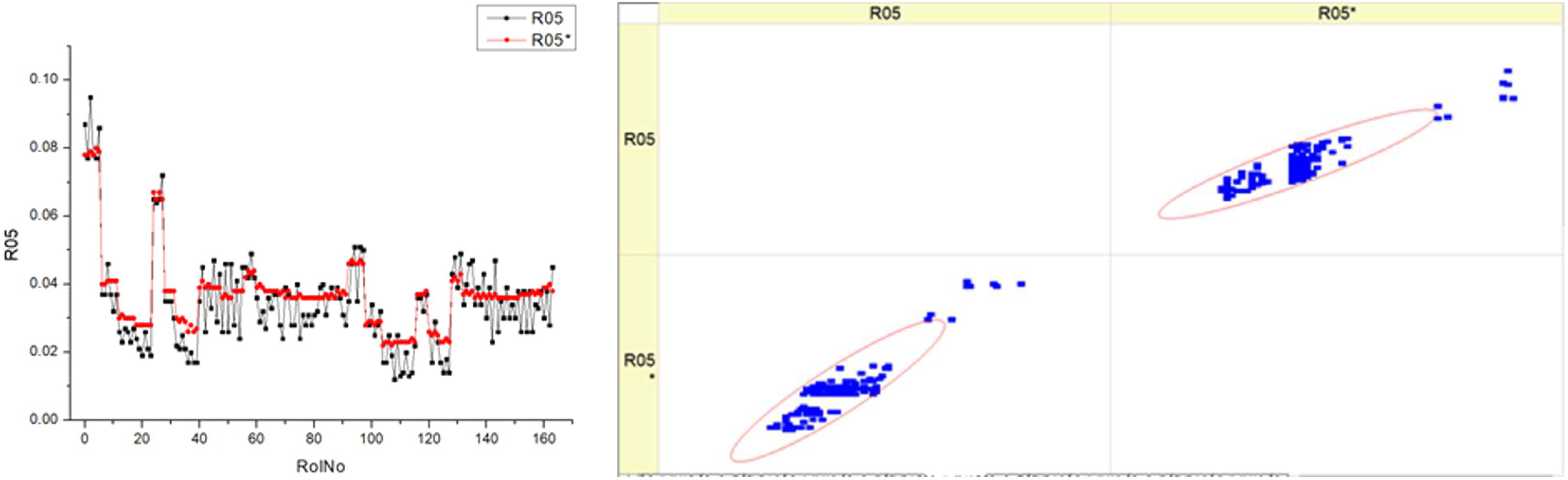
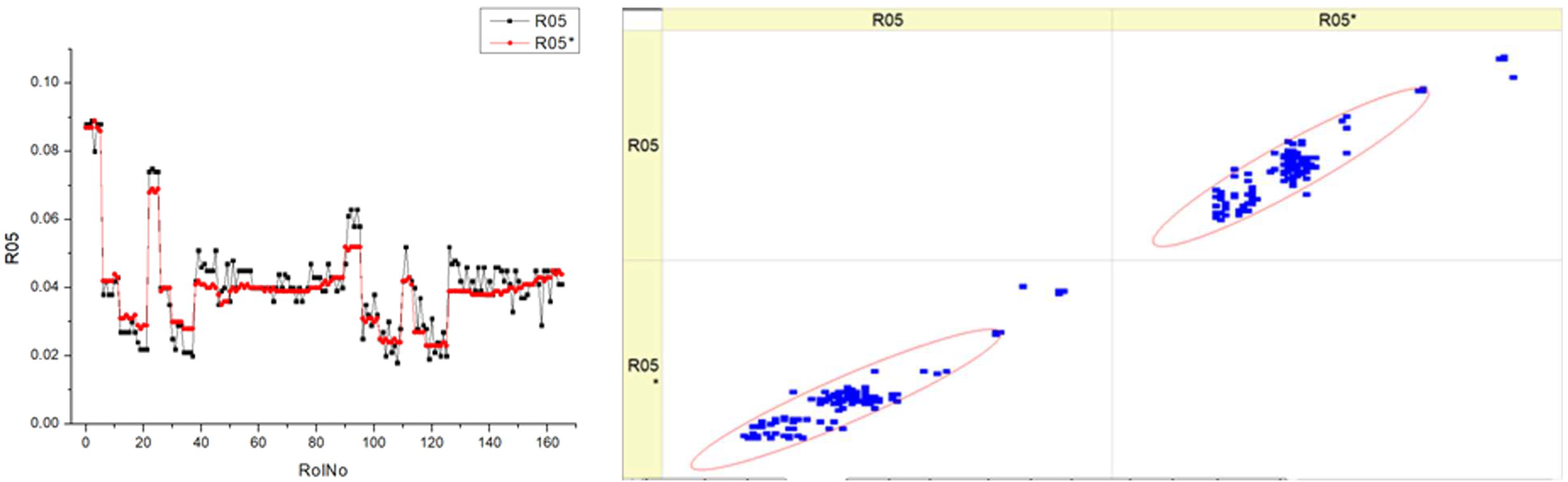
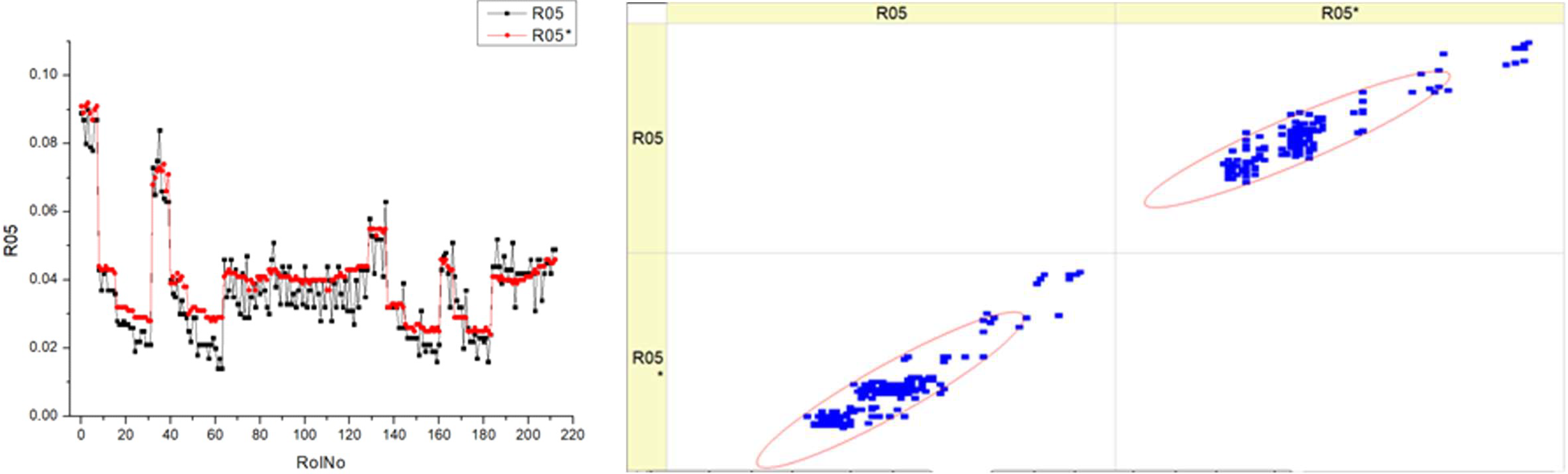
Specific hydrocarbon emissions (SHC) decrease significantly with increasing engine load (Table 14), as the concentration of HC in the exhaust gas demonstrates less of an increase as the load increases. The change in the EGR ratio does not significantly affect the change in SHC, as the O₂ concentration is quite high, and the combustion-inhibiting effect of EGR is compensated by the higher temperature at the start of combustion. Increasing the concentration of HVO in the fuel mixture results in a negligible change in SHC emissions, as the higher-quality atomization of lower-viscosity fuels with higher HVO concentration is likely to be canceled out by the earlier start of ignition at lower temperatures due to a higher cetane number. The predicted SHC emission rates are more stable than the experimentally determined ones because the gas analyzer data were not stable at low concentrations of HC pollutants.

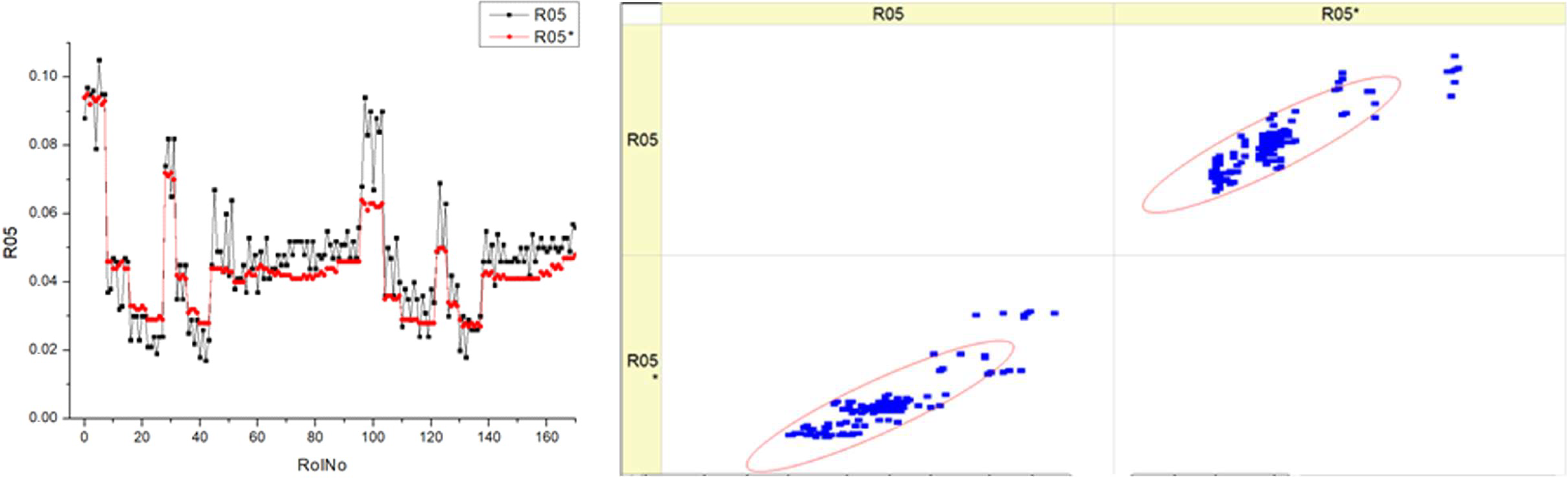
Table 14, labeled R05, displays the SHC. The histograms on the left side illustrate the distribution of the SHC parameter for each fuel type overt a range of runs or measurements (RunNo). Each fuel type has two sets of data, labeled R05 and R05*, which may indicate distinct experiments and circumstances. The distribution patterns of SHC throughout the runs are shown, with some runs exhibiting several peaks while others display wider dispersion. The scatter plots on the right juxtapose the projected SHC values with the actual measured values, where the diagonal line signifies flawless forecast accuracy. A denser clustering of points along the diagonal line suggests more precision in forecasts. The scatter plots illustrate that the accuracy fluctuates across various fuel types.

The histograms indicate that the SHC parameter fluctuates with different fuel types, suggesting that the composition of the fuel may impact the efficiency of hydrocarbon consumption.

The scatter plots illustrate the efficacy of the prediction model. The fluctuating distance of points from the diagonal line implies that the model’s capacity to precisely forecast SHC is influenced by the fuel type. Upon examining the scatter plots, it seems that greater fuel types may be associated with a tendency towards enhanced forecast accuracy. This may be deduced from the concentration of data points in close proximity to the diagonal line. The existence of two datasets for each fuel type (R05 and R05*) suggests the strength of the measuring techniques or the consistency of the model’s ability to forecast accurately in various experiments or circumstances.

Both kinds of graphs may demonstrate the influence of the fuel mixture on the engine’s particular hydrocarbon consumption and the accuracy of a model in predicting this consumption.

Essentially, this image illustrates the correlation between the actual performance of an engine, measured in terms of SHC, and the accuracy of a predictive model in forecasting this performance across various fuel mixes. The discrepancies seen in the histograms and the patterns of clustering in the scatter plots indicate that both the actual consumption of hydrocarbons in the real world and the ability to anticipate this consumption are influenced by the particular kind of fuel being utilized.

The formation of nitrogen oxides (NO_x) during combustion in a compression ignition engine is mainly influenced by the combustion temperature. The combustion temperature rises and the NO_x concentration in the exhaust gas increases with increasing engine load (Table 15) as more fuel is injected into the cylinder per cycle, and, with the advancing SOI, the heat release peak happens in a smaller combustion volume. Advancing the SOI due to a lower temperature in the cylinder at the start of fuel injection prolongs the ignition delay, which results in more fuel injected in the delay phase and more heat released once combustion starts. Increasing the EGR ratio reduces the combustion temperature and NO_x emissions by returning combustion products (CO₂ and H₂O) to the cylinder, which reduces the O₂ concentration and slows down the combustion speed. Increasing the concentration of HVO in the fuel mixture should reduce the NO_x concentration as the cetane number of the fuel increases (Table 3), and faster ignition should reduce the ignition delay and temperature rise. However, increasing the HVO content of the fuel did not result in a noticeable reduction in NO_x concentrations, as the engine was warmed up to operating temperature and the increase in the cetane number did not have a significant effect. In the case of the NO_x assessment, the measurement data were significantly higher than the gas analyzer’s lower measurement limit, and the NO_x values were stable for each engine’s operating mode. It can be seen visually that the predicted NO_x concentrations are close to the experimental values.

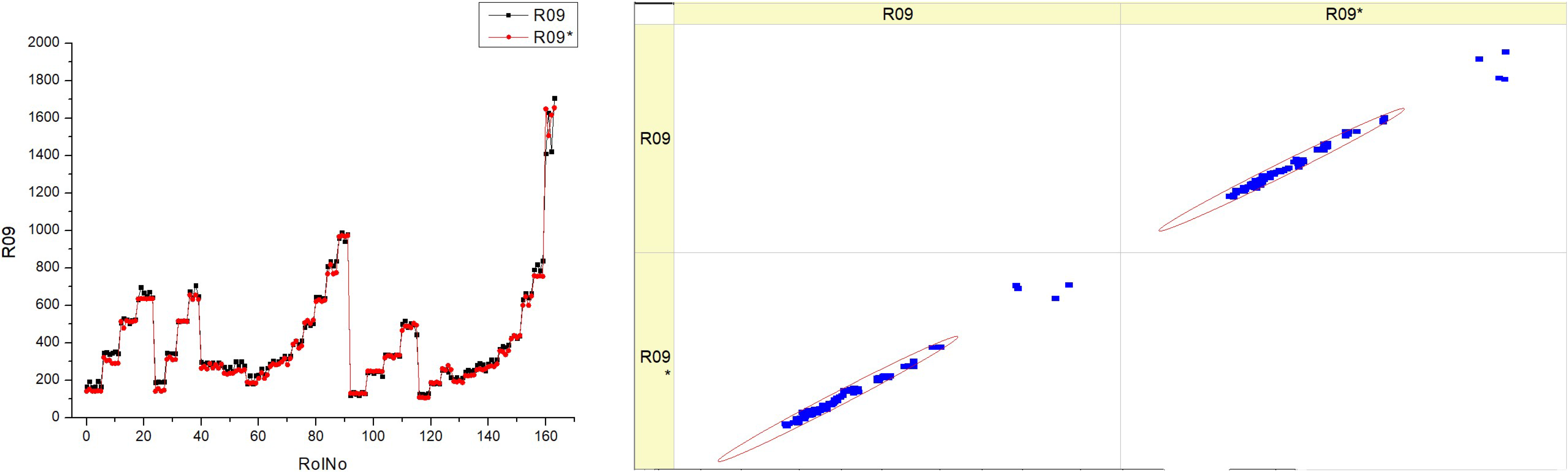
Table 15 provides information on the NO_x concentration in the exhaust gas during the experimental tests and the prediction of this indicator. These emissions may serve as an indicator of the efficiency of combustion and the influence on the environment. The histograms on the left show the frequency distribution of NOx levels throughout a series of runs (RunNo). Each histogram displays two sets of data, R09 and R09*, which may be used to compare various testing circumstances, engine settings, or techniques of measurement.

The histograms exhibit distinct variations in form for each fuel type, reflecting diverse frequencies and ranges of NOx concentration. This observation provides insight into the fluctuations in nitrogen oxide levels resulting from the utilization of various fuels.

The scatter plots on the right side illustrate the comparison between the anticipated NOx levels and the actual measured values. The diagonal line indicates a precise alignment between the expected and actual values. The presence of point clusters along this diagonal line indicates a high level of prediction accuracy. The scatter plots exhibit varying point distributions corresponding to different fuel types, suggesting that the model’s forecast accuracy is influenced by the amount of fuel. The histograms illustrate the variability of NOx concentration over different runs and fuel types, indicating that fuel composition has a substantial influence on NOx production.

The scatter plots depict the precision of a prognostic model for NOx concentration. The proximity of the points to the diagonal line directly correlates with the level of accuracy in the forecasts. For some types of fuel, there is a concentrated group of data points that are closer to the diagonal, indicating a higher degree of accuracy in predicting their performance. The scatter plots suggest that there is a correlation between higher fuel types and more accurate forecasts. This is supported by the observation that there is a greater concentration of data points along the diagonal line for HVO40 and HVO50.

The presence of two datasets (R09 and R09*) for each fuel type indicates the coherence of the emissions data under various testing settings or the dependability of the used prediction models. Both kinds of charts presumably demonstrate the influence of fuel composition on NOx concentration and the difficulty of forecasting these emissions for various fuel types.

To summarize, the image illustrates a comparison between the amounts of NOx concentration and the forecast accuracy of a model for various fuel compositions. The histograms and scatter graphs illustrate the variations in NOx concentration, taking into account both the number of runs and the kind of fuel used. These variations have consequences for engine performance, fuel economy, and environmental compliance.

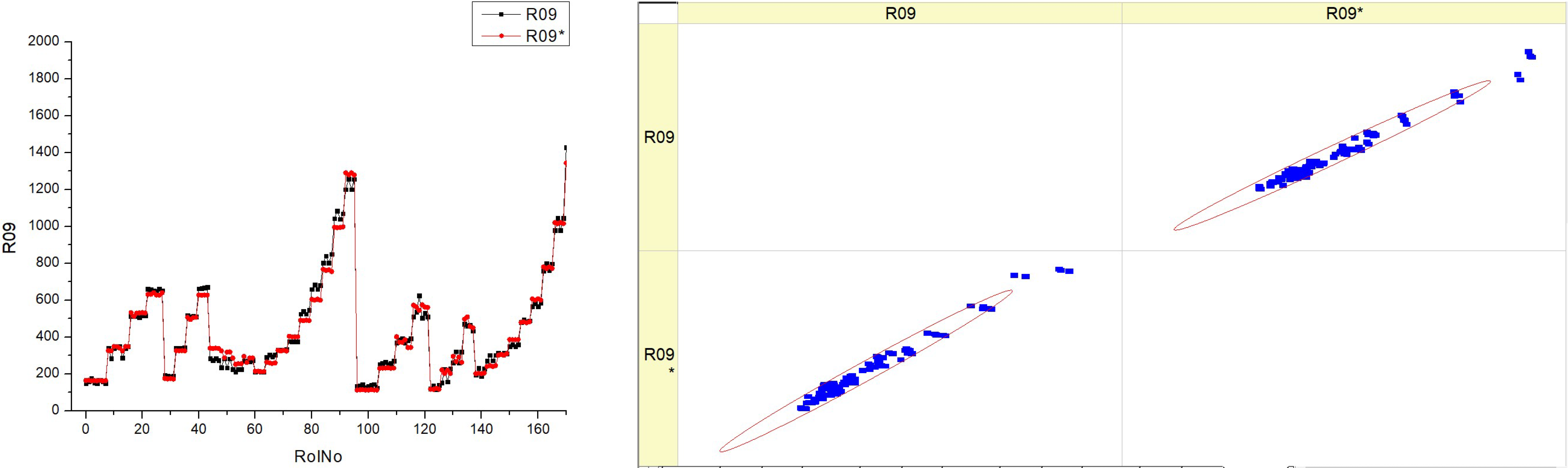
When comparing Figures R04 and R09, we are analyzing two distinct tables from the research. Each table most likely represents the distribution of a separate parameter related to engine performance and emissions. R04 corresponds to a parameter labeled “SNOx”, whereas R09 corresponds to “NOx”. The histograms for both R04 and R09 exhibit various distributions across different fuel types. These distributions differ in terms of their range and the points at which they occur most often. R04 has a higher frequency of certain SNOx values, while R09 shows a notable variability in NOx levels over the runs.

Each table has two sets of histograms (R04 and R04*, R09 and R09*) that represent various experimental settings, duplicate measurements, or comparisons between distinct datasets. Both R04 and R09 exhibit fluctuation across runs, indicating potential alterations in the parameter as a result of engine operating circumstances or the kind of fuel used.

The scatter plots in both R04 and R09 are used to juxtapose the projected values with the actual measured values for their respective parameters. The scatter plots for R04 and R09 exhibit different levels of prediction precision, as demonstrated by the proximity of the data points to the diagonal line. Both examples exhibit a discernible pattern where scatter plot points for higher fuel types (HV040 and HV050) tend to cluster in proximity to the diagonal line, indicating enhanced precision in forecasts for higher fuel types. Both R04 and R09 exhibit internal consistency within each fuel type, as shown by two sets of data points (R04 with R04*, R09 with R09*) that indicate the accuracy of the model’s predictions in relation to the actual measurements.

The observed values and fluctuations in the histograms indicate that the parameters exhibit varying degrees of sensitivity to changes in fuel and engine conditions. The concentrations of NOx may significantly fluctuate depending on the temperature of combustion. On the other hand, SNOx readings may be more closely associated with the chemical makeup of the fuel. Higher HVO concentration in a fuel blend seem to result in improved performance of the prediction model for both parameters.

Both of the histograms for R04 and R09 show distributions with many modes, and the scatter plots for both indicate that the model’s accuracy varies over various fuel types.

Comparing Tables R04 and R09 demonstrates that while separate parameters (SNOx and NOx) exhibit diverse distribution patterns and consequences, the fundamental trends in model prediction across different fuel types and the consistency across datasets are similar. Additionally, the accuracy of prediction models may vary based on the specific parameter and fuel type being examined.

The specific emissions of nitrogen oxides (SNO_x) provide more detailed information compared to the NO_x concentration. Table 16 shows that SNO_x increases significantly less than NO_x with increasing engine load. However, as the fuel injection advance increases, SNO_x emissions increase as much as the NO_x concentration. SNO_x, like NO_x, is only reduced by increasing the EGR ratio at a constant engine load. Increasing the concentration of HVO in the fuel mixture did not significantly change the SNO_x emission because the engine was warmed up during the tests and the higher cetane number of HVO had a negligible effect. Due to the high accuracy of the measurements and the mathematical processing of the data, we can visually see a quite accurate prediction of the SNO_x emissions at different engine operating modes.

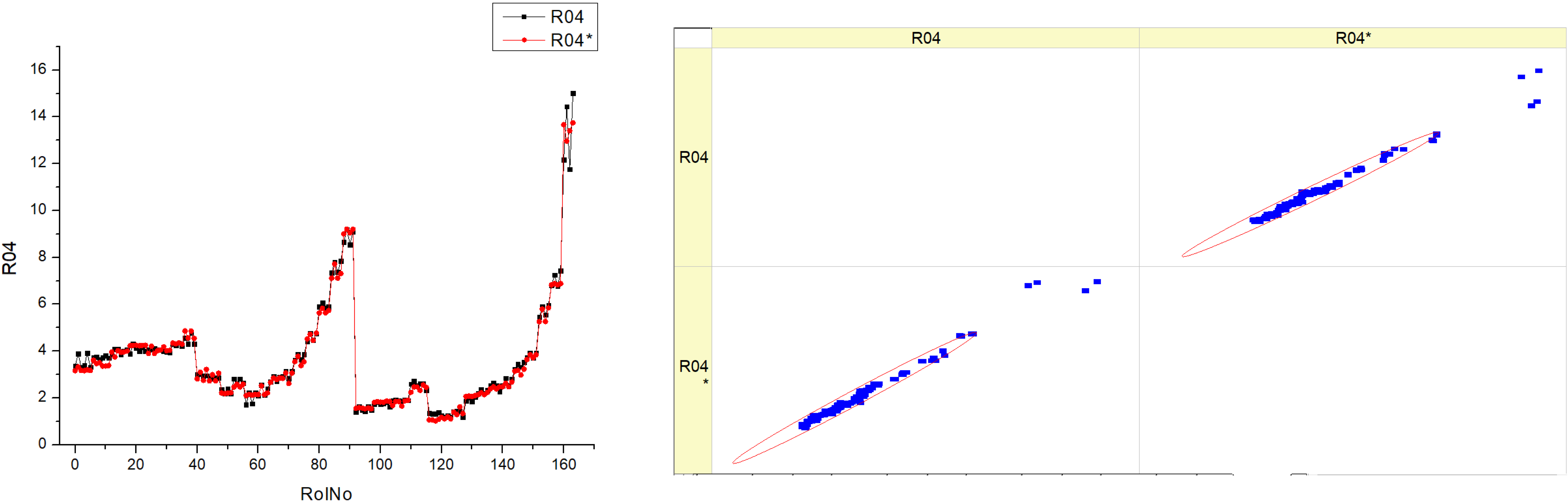
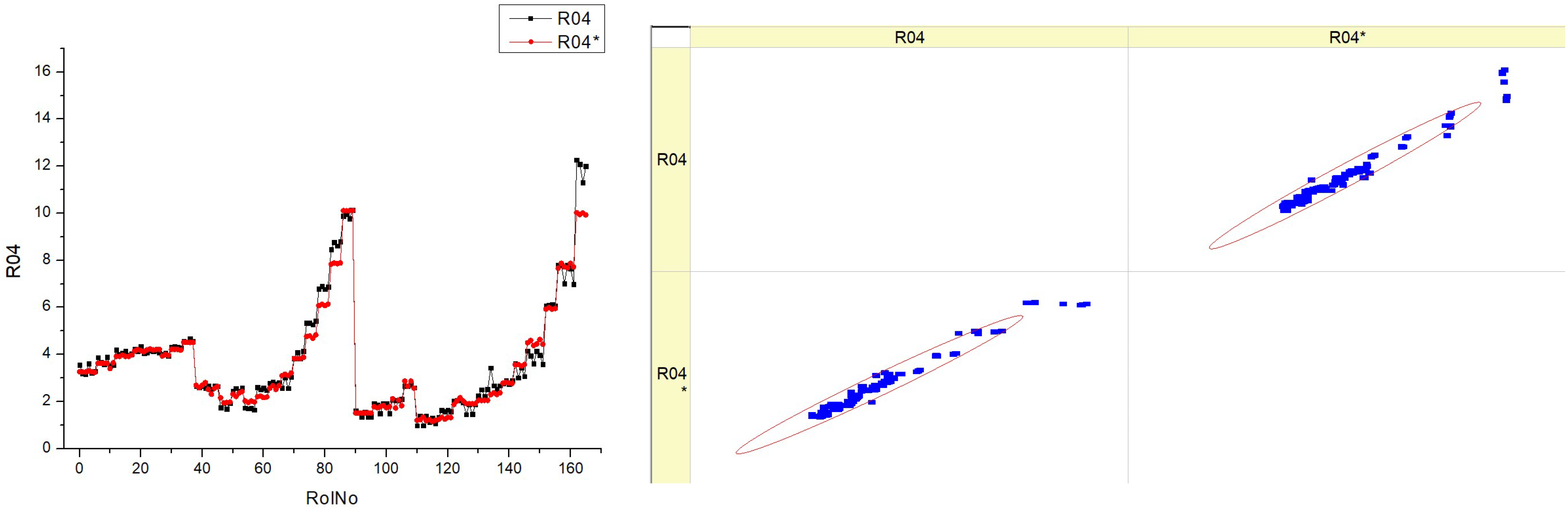
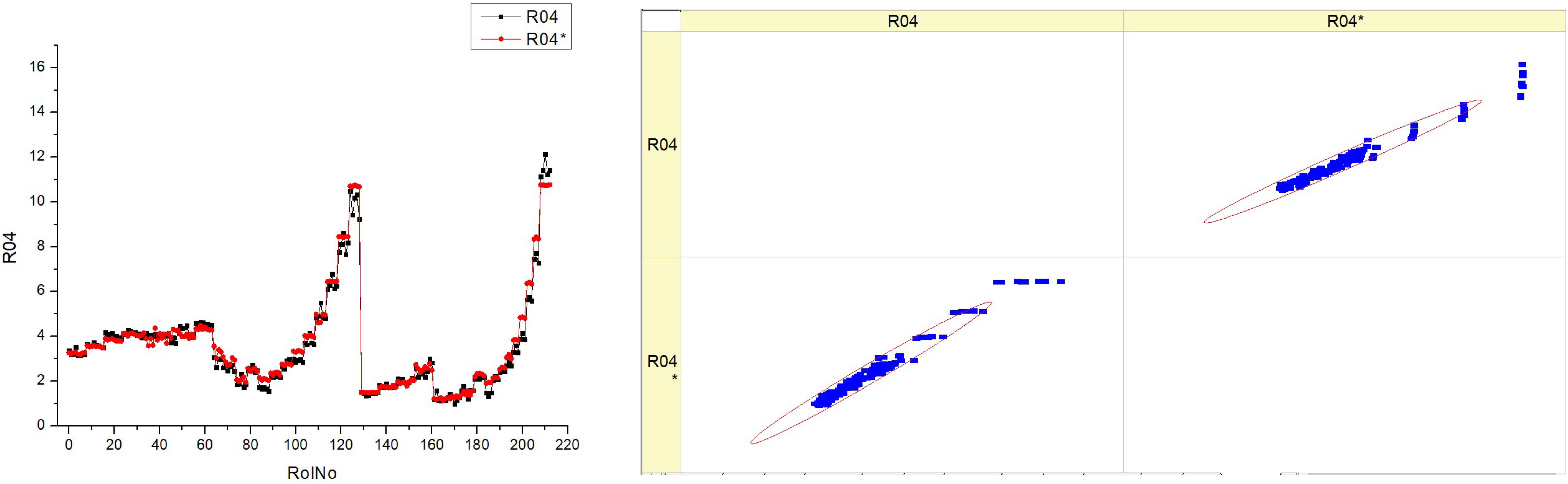
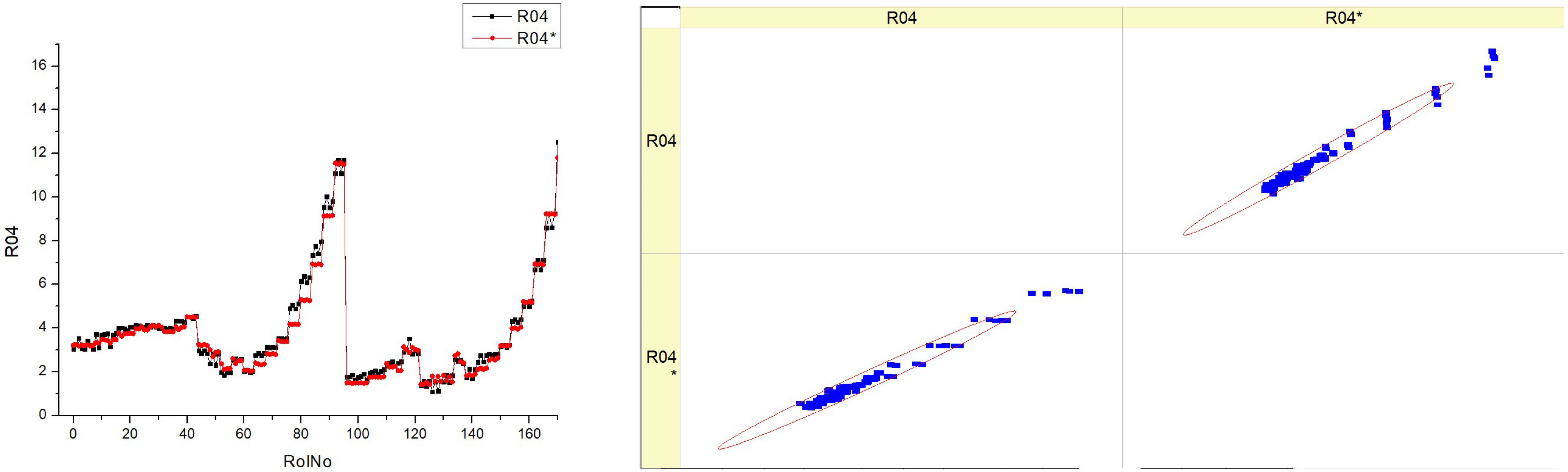
Table 16 (R04) displays histograms and scatter graphs representing the data for SNOx. The histograms on the left show the distribution of the SNOx parameter over several runs, identified as RunNo. Each histogram has two lines, denoted as R04 and R04*, which may indicate distinct situations, such as before and post alteration, or different measurement methodologies.

The distribution patterns of SNOx vary depending on the fuel type. Some patterns exhibit significant fluctuation, while others have more distinct peaks, indicating certain ranges with increased frequency.

The scatter graphs on the right juxtapose the projected values of SNOx with the actually measured values. Points that lie on the diagonal line indicate a flawless forecast. The deviation of the dots from the diagonal line indicates the variability in the accuracy of predictions. A denser grouping along the line would indicate a model that is more precise.

The histograms demonstrate that the SNOx parameter’s behavior varies depending on the kind of fuel used, as shown by the distinct frequency and distribution of values.

The scatter plots illustrate the efficacy of the model in forecasting SNOx. There are several levels of accuracy seen across the fuel kinds, with some levels exhibiting points that nearly match with the diagonal, indicating improved predictability.

Upon examining the scatter plots, it seems that there is a potential correlation between higher fuel types, such as HVO40 and HVO50, and a denser clustering of data points along the diagonal line. This suggests that the predictive model may exhibit improved performance with these fuel compositions.

The inclusion of R04 and R04* in each plot suggests that the parameter’s distribution is resilient or that the predictive model’s accuracy remains stable across many tests or settings.

The aggregated data from the histograms and scatter plots may provide insights into the impact of fuel composition on the SNOx parameter and the prediction model’s accuracy in estimating it.

Essentially, this figure compares the actual measurement distributions of a certain parameter with the precision of a prediction model for various fuel mixes. The observed differences in histogram patterns and the grouping of data points in the scatter plots indicate that the SNOx parameter and its model prediction are affected by the specific kind of fuel being burned.

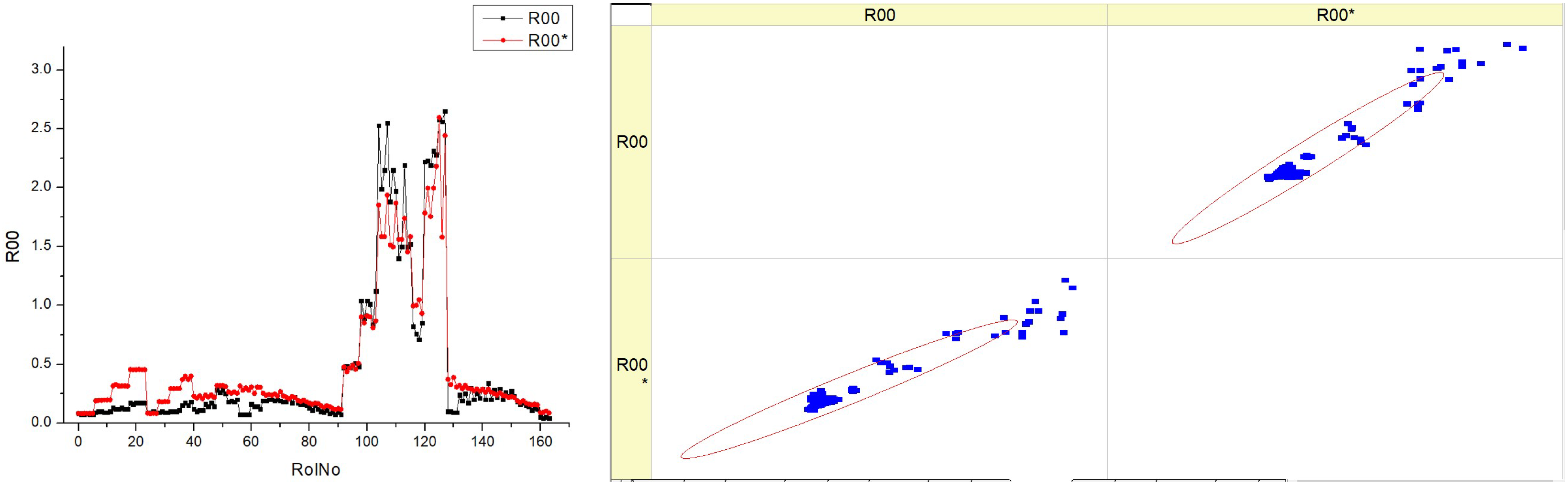
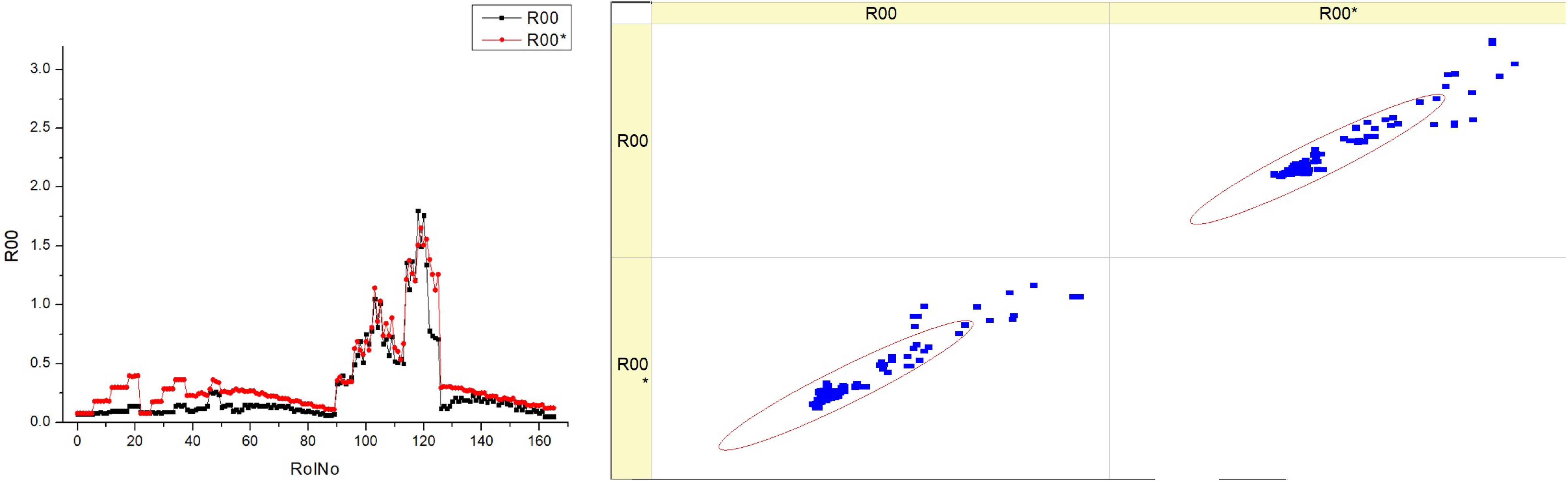
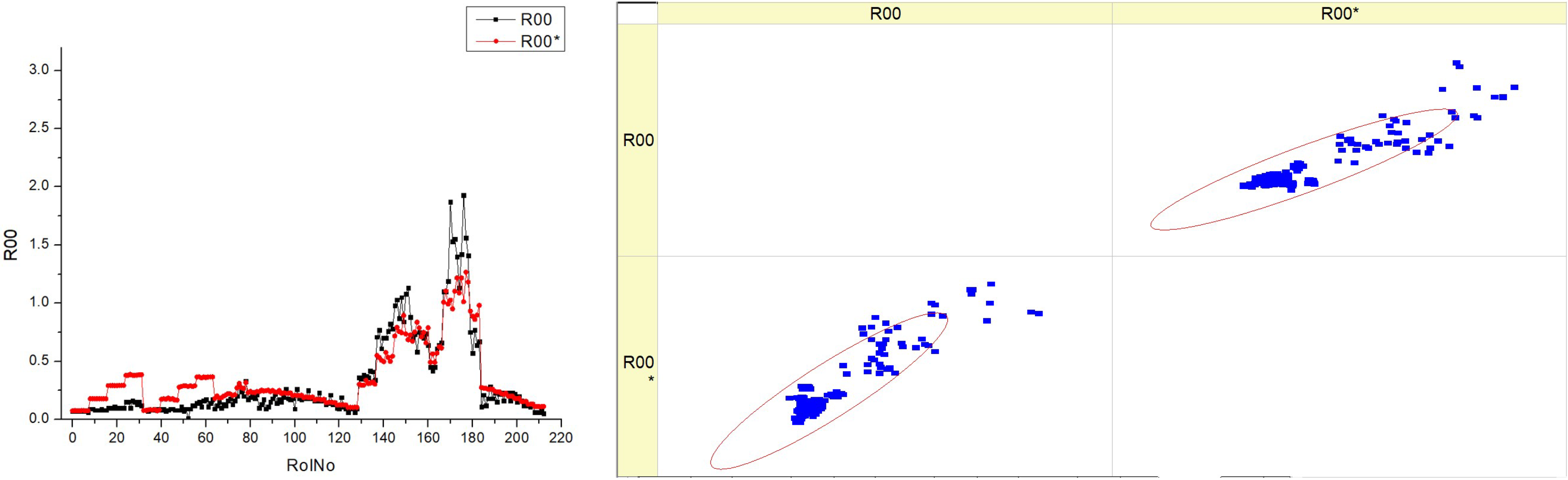
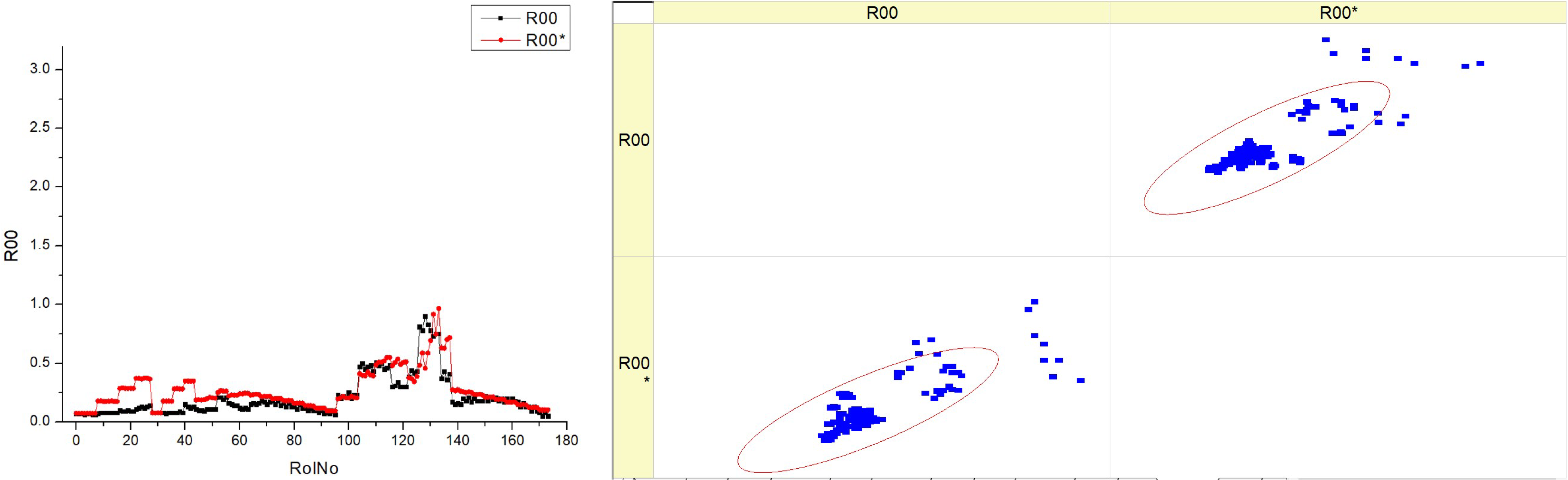
The smokiness is one of the most important indicators of engine pollution, which depends on the quality of combustion and correlates with the emission of particulates. An experimental study has shown that the smokiness increases at a low intensity with increasing engine load when the EGR is closed (Table 17). Increasing the EGR intensity at constant load also leads to a limited increase in smokiness. When the EGR is open, the increase in smokiness with increasing load is much more intense, as the excess air is reduced more significantly, and the returned combustion products additionally suppress combustion.

Smokiness decreases with advanced SOI, as combustion takes place at a higher temperature. These trends are typical for all fuel blends, but with increasing concentrations of HVO, smokiness is lower, especially at peak pollution points. Research shows that HVO reduces smokiness by reducing the carbon content and increasing the hydrogen content of the fuel, while the lower viscosity of the fuel improves the quality of the atomization. When analyzing the prediction of the smokiness, we can see that the increase in smokiness with increasing engine load without EGR is much higher than the experimental results. This inaccuracy in the prediction is likely due to the large increase in smokiness observed in the experiment as the load increases with EGR operation.

The histograms indicate that the smokiness parameter displays distinct patterns at various fuel types, which may be attributable to the composition or characteristics of each fuel type.

The scatter figure illustrates the correlation between different fuel types and the accuracy of the model’s predictions for smokiness. The scatter plot of dots in relation to the diagonal line indicates the model’s performance, which exhibits variation based on the fuel type. There is a possible pattern in which scatter plots of higher fuel types (HVO40 and HVO50) exhibit a greater concentration of data points along the diagonal line compared to lower fuel types (HVO10 and HVO30). This suggests that the predictive model exhibits superior performance when the fuel types are greater.

The inclusion of R00 and R00* data in every panel indicates that the measurements are replicable or that there is a comparison between two distinct models. The histograms and scatter graphs suggest a correlation between the smokiness parameter and the fuel type. For example, an increased fuel type might be associated with a more consistent smokiness factor, resulting in improved model accuracy.

Essentially, the graphic illustrates the distribution of a smokiness parameter across various fuel types and the predictive accuracy of a model for this parameter. There are observable differences in the distributions of the histograms and the density of clusters in the scatter plots, suggesting that both the behavior of the parameter and the prediction capacity of the model are affected by the fuel type.

5. Discussion

Figure 4 displays a set of subplots, each representing a variable labeled from R00 to R09, illustrating the fluctuations of their Pearson correlation coefficients in connection to four distinct fuel types: HVO10, HVO30, HVO40, and HVO50. The Pearson correlation coefficient is a statistical metric that quantifies the magnitude and direction of the association between two variables. In this case, it is being used to demonstrate the linear link between each R parameter and the specific kind of fuel utilized.

In order to elucidate the variations of each R parameter with respect to the fuel type, we systematically examine each parameter as it is shown in the figure. The R00 parameter has a robust positive correlation with fuel types HVO10, HVO30, and HVO40, as shown by coefficients that are either equal to or extremely close to 1. However, there is a noticeable reduction in correlation with HVO50, as the coefficient decreases dramatically, indicating a weaker positive link. The correlation for the R01 parameter stays consistently strong across all four fuel types, indicating that changes in gasoline type have little impact on the variable R01. Like R01, R02 has a consistently strong correlation with the fuel types and does not display any significant variation among the various fuels.

R03 has a strong or almost perfect association with the first three fuel types, but it shows a somewhat reduced, although still very high, correlation with HVO50. The correlation between the R04 variable and the different fuel types is consistently high, suggesting a strong, positive, linear association independent of the specific fuel type. R05 has a strong association with all fuel types, with no noticeable variation as the fuel type varies. The correlation coefficient for R06 shows a notable decrease when comparing the first three fuel types, which have a strong or almost perfect connection, to HVO50. This suggests that the association between R06 and HVO50 is less strong.

In terms of R07, this parameter exhibits a significant association with the first three fuel types. Similarly to R03 and R06, the correlation weakens when HV050 increases, but it still stays significantly positive. The correlation with R08 stays consistent and very strong across all fuel types. Finally, R09 has a flawless or almost flawless correlation with all fuel types, suggesting a very robust positive linear association that remains consistent regardless of the fuel type.

To summarize, the majority of R parameters have a significant positive connection with fuel types, suggesting that if one variable grows, the other also tends to increase. Nevertheless, the correlation of the R00, R03, R06, and R07 parameters shows a small decline when the fuel type is HVO50, indicating that these characteristics have a weaker positive association with the HVO50 fuel type compared to the other three fuel types. This suggests that the shift to a gasoline with greater viscosity (assuming HVO50 has higher viscosity based on its naming practice) may have an impact on these particular parameters, perhaps altering the connection indicated by the Pearson correlation coefficient.

The advantages of this method are summarized here. Firstly, ANNs can provide a self-regulation procedure for data without requiring specifical statistical approaches. Decreasing the significance of data “out of context” is one of the main important features of ANN. Secondly, for modeling complex systems when relations between parameters are hidden due to a chaotic nature, only a learning procedure through epochs (from several hundred thousand to several hundred million) allows for highlighting such inner dependencies (to handle unseen data after the learning process). Due to this, complex mathematical considerations are not necessary.

The main innovation points of this research can be formulated as follows. The demonstration of ecological predictions for different regimes of diesel engine was accomplished using burning chemistry approaches (in a purely experimental way, which is quite expensive) as well as ANN facilities (a simulation using understandable and adaptive methods, which is a cheap way). We decided to use ANNs due to the possibility to learn the nonlinear relationship between inputs and outputs, making them suitable to represent the amount of outcomes (chemical parameters) related to the technical parameters of diesel engines and the chemical parameters of fuel compounds belonging to the different mixtures. According to the literature review, relations of such a type are fragmental (dedicated to the unique case, unique engine, unique fuel, etc.), and they are not presented in routine expressions for large sets of different outcomes. In our case, solving real-world problems (prediction of outcomes for different mixtures of fuels) by means of ANNs is grounded in a non-traditional approach that works very efficiently.

6. Conclusions

• The work demonstrates the efficacy of machine learning models in precisely predicting diesel engine emissions, achieving a high R² value of 0.984. The model’s capacity to acquire and adapt effectively is essential for reliable forecasts in practical situations. Nevertheless, the first high error rates might be attributed to overfitting or the insufficiency of the training data. As the training advances, the intricate models tend to attain a stable state, suggesting that attaining an optimal result requires a careful equilibrium between the complexity of the model and the depth of the training.
• This study emphasizes the need to consider fuel volatility when constructing prediction models for engine emissions. The model’s capacity to adjust to diverse fuel types while upholding precision is crucial for deploying applications in different geographical areas and regulatory situations. This study used histograms and scatter plots to illustrate the dispersion and precision of predictions at various fuel levels, thus enhancing trust in the model’s outcomes.
• The model’s capacity to precisely predict CO₂ and NOx emissions in various situations underscores its use in environmental monitoring and compliance with emission regulations. The reliability and consistency of the prediction model are assessed by analyzing results from several datasets, including R06 and R07. This revelation has profound ramifications for the management of diesel engines, the optimization of engine performance, the selection of suitable fuel, and the development of operational strategies that minimize environmental damage while guaranteeing efficiency.