Article

Validation Challenges in Data for Different Diesel Engine Performance Regimes Utilising HVO Fuel: A Study on the Application of Artificial Neural Networks for Emissions Prediction

by
Jonas Matijošius
1,2,*,
Alfredas Rimkus
1,3 and
Alytis Gruodis
4
1
Department of Automobile Transport Engineering, Technical Faculty, Vilnius College of Technologies and Design, Olandu Str. 16, LT-01100 Vilnius, Lithuania
2
Mechanical Science Institute, Vilnius Gediminas Technical University-VILNIUS TECH, Plytinės Str. 25, LT-10105 Vilnius, Lithuania
3
Department of Automobile Engineering, Faculty of Transport Engineering, Vilnius Gediminas Technical University-VILNIUS TECH, Plytinės Str. 25, LT-10105 Vilnius, Lithuania
4
Faculty of Public Governance and Business, Mykolas Romeris University, Ateities Str. 20, LT-08303 Vilnius, Lithuania
*
Author to whom correspondence should be addressed.
Machines 2024, 12(4), 279; https://doi.org/10.3390/machines12040279
Submission received: 9 March 2024 / Revised: 15 April 2024 / Accepted: 18 April 2024 / Published: 21 April 2024

Abstract

:
Artificial neural networks (ANNs) provide supervised learning via input pattern assessment and effective resource management, thereby improving energy efficiency and predicting environmental fluctuations. The advanced technique of ANNs forecasts diesel engine emissions by collecting measurements during trial sessions. This study included experimental sessions to establish technical and ecological indicators for a diesel engine across several operational scenarios. VALLUM01, a novel tool, has been created with a user-friendly interface for data input/output, intended for the purposes of testing and prediction. There was a comprehensive collection of 12 input parameters and 10 output parameters that were identified as relevant and sufficient for the objectives of training, validation, and prediction. The proper value ranges for transforming into fuzzy sets for input/output to an ANN were found. Given that the ANN’s training session comprises 1,000,000 epochs and 1000 perceptrons within a single-hidden layer, its effectiveness can be considered high. Many statistical distributions, including Pearson, Spearman, and Kendall, validate the prediction accuracy. The accuracy ranges from 96% on average, and in some instances, it may go up to 99%.

1. Introduction

Many technical and industrial problems [1] (predicting output parameters based on predicted or implied influencing factors) are addressed and solved by choosing the correct approximation function and evaluating the nature of the correlation [2]. However, this type of task quickly becomes too difficult when (a) there are many parameters that potentially influence the phenomenon, (b) the correlation is weak and insignificant, and (c) the previous approximations of a linear nature do not work or work with a large error. Many natural processes in complex nonlinear systems occur at very low speeds [3]. Over time, the process accelerates and approaches saturation [4]. In this case, it is possible to use artificial intelligence implementations that can solve atypical, incorrect, or large-scale sampling tasks.
An artificial neural network is a basic network consisting of an input layer, an output layer, and one or more intermediate neuron layers [5]. The main advantage of this network is that it evaluates input patterns after training [6]. For such a network, supervised learning can be organized based on examples where input and output are linked by an event, or, in other words, a cause forms an effect (for example, experimental results of physical phenomena or function values obtained by an unknown formula, etc.). The essence of ANN training is that the desired output can be produced within a given error tolerance.
Artificial intelligence (AI) refers to the simulation of human intelligence in computer systems designed to solve problems in a human way [7]. AI systems are designed to analyze data, recognize patterns, make decisions, and improve over time through iterative learning processes or decision-making. Artificial intelligence can be used to monitor and manage resources [8], optimize energy consumption [9], and predict environmental changes to help address climate-related issues [10]. AI’s main realization is ANN, which is based on the properties of biological neural networks. The structure and activity of the animal brain are modelled as a mathematical network of interconnected nodes (perceptron) divided into several layers: input, hidden, and output.
Several fundamental textbooks are interesting for understanding the newly developed paradigms of artificial neural networks. Zurada [11] defines the focus of the study of artificial neural systems. “Artificial neural systems are physical cellular systems that can acquire, store, and utilise experiential knowledge”. Multilayer feedforward networks are presented and discussed in a user-friendly form. Rabunal et al. [12] described the processes of brain learning and the corresponding mathematical operations built up according to the analogy to brain activity. According to Rabunal, two main advantages of ANN are adaptive learning and fault tolerance. Adaptive learning is the ability to learn to perform tasks based on a training session that consists of selecting data specific to the task. Fault tolerance refers to the ability of a network to maintain its previous functions after a partial destruction of the network results in a corresponding performance degradation. Goodfellow et al. [13] presented the paradigm of deep learning, which allows a computer to construct complex concepts from simpler concepts. A significant example of a deep learning model is a multilayer perceptron (MLP). A mathematical function in the form of MPL associates some set of input values with output values. Torres-Sospedra [14] presented and discussed several design methods that are important for expanding the ANN. Lou [15] presented and discussed the abilities of neural networks, which belong to a subfield of machine learning.
Implementations of ANN for technical purposes (control and prediction of exhausts) were described in a series of contemporary publications.
Firstly, problems of data sampling must be solved within the framework of Big Data. Li et al. [16] presented a study that introduces a high-throughput fuel screening approach for early property-oriented fuel design in internal combustion engines. This process includes Tier 1 fuel physicochemical property screening and Tier 2 chemical kinetic screening. Ahmad et al. [17] claim that machine learning (ML) is one of the major driving forces behind the fourth industrial revolution. This study reviews the ML applications in the life cycle stages of biofuels, i.e., soil, feedstock, production, consumption, and emissions. The ML applications in the production stage include the estimation and optimization of quality, quantity, and process conditions. Usman et al. [18] presented the ANN-2HL-15 N model, among six trained models, which demonstrated exceptional efficiency in predicting operational effectiveness and discharge levels in small-scale single-cylinder SI engines. Its performance under optimal operating conditions improved emissions, CO, and HC emissions, as well as combustion. The combination of ANN and RSM promotes sustainable industrialization, conscientious consumption, and ethical production patterns, supporting SDGs 9 and 12.
Secondly, the implementation of ANN must be realized in a standalone manner as well as in close collaboration with other AI algorithms. Deng et al. [19] described the possibilities of ANN for engine application purposes (testing and diagnostics). Several models, such as the basic model for a fuel path control system, ANN to represent air flow rate, the Nox prediction ANN model, and the smoke prediction ANN model, are presented and estimated. Xing et al. [20] examine various aspects of control related to biodiesel production. Identifying unknown nonlinear relationships between the system input and output data is not easy. Therefore, accurate and swift modelling instruments like M) or AI are necessary to design, handle, control, optimize, and monitor the system. Aliramezani et al. [21] presented ICE modelling for meeting emission regulations and minimizing fuel consumption. ML can tackle these challenges by addressing areas such as combustion knock detection, emission formation modelling, mode transition, combustion noise modelling, instability control, ICE optimization, and component fault diagnostics. Zhang et al. [22] studied a single model to simulate CO2, CO, and Nox emissions from biodiesel combustion in compression ignition engines. The authors used three machine-learning tools to model the complex MIMO-type regression problem. The biodiesel source’s physical features were found to be the best, and the MLS-SVR was the most reliable tool for estimating emissions. Khac et al. [23] present ANN-based models for estimating nitrogen oxide and carbon dioxide emissions from a maritime diesel engine’s in-cylinder pressure. Using data from a four-cylinder engine, the models show MLP has higher accuracy than RBF, despite the engine’s conventional nature and generalization to avoid overfitting. Žvirblis et al. [4] described the optimal prediction model for exhaust emission parameters. The optimal model predicted most engine emissions with high accuracy, but NOX remained unpredictable. The interaction between injection timing and sound pressure remained statistically relevant. Engine emissions from the DF and HVO50 groups were not statistically different, with higher trends for PM, CO, HC, and NOX in the DF group. Injection timing had more influence on the distribution of emission parameters.
The problem of an algorithm suitable for ANN could be treated as a classical problem due to the impossibility of strong systematization of the calculation routine. Venkatesh et al. [24] studied the usage of 29 machine learning algorithms to estimate engine emissions in dual-fuel engines with hydrogen and diesel. The most effective algorithms included pace regression, radial basis function regressors, multilayer perceptron regressors, k-nearest neighbor, and alternating model trees. The J48 decision tree algorithm was used to establish the relationship. Leo et al. [25] used the random forest algorithm for evaluating the emissions of WCOB biodiesel with Al2O3 and FeCl3 in a gasoline-premixed HCCI-DI engine. Results showed lower BTE, a 54.17% reduction in HC emissions, and decreased carbon dioxide emissions. Al2O3 nano-additives reduced smoke emissions by 30.4%, 24.8%, and 23.65%, respectively. Williams et al. [26] studied the random forest regression and neural network models to predict the rate-of-injection (ROI) profiles of a diesel injector. The neural network model performed better than the random forest model. Future work could include considering pressure, parameters, and larger input data, as well as focusing on ROI input in CFD simulations.
For prediction purposes, ANN is generally considered the most profitable model. Bekesiene et al. [27] examined complex stress factors in military service using an ANN model. Maximum accuracy was obtained using a multilayer perceptron neural network (MLPNN) with a 6-2-2 partition. The best ANN model was determined as the one that showed the smallest cross-entropy error. Jovanovic et al. [28] discussed how to implement neural networks in different programming languages. Here, the implementation of an arbitrary neural network in Java is examined. Godwin et al. [29] studied ANN and Ensemble LS Boosting to predict the combustion, performance, and emission parameters of an internal combustion engine using gasoline and ethanol blends. The ANN model demonstrated near-perfect precision in predicting key engine parameters, while the Ensemble LS Boosting model showed superior congruence with experimental engine parameters. The ensemble nature, resistance to overfitting, and optimized hyperparameters contributed to the Ensemble LS Boosting model’s outstanding performance.
This work is based on experimental studies of the combustion characteristics, energy, and ecological indicators of a diesel engine carried out at Vilnius Tech.
The main aims of this work could be formulated as follows:
  • To construct an advanced tool with a user-friendly interface for data input and output facilities to provide simulations and predictions of exhausts in outcomes.
  • For an artificial neural network, construct the interfaces for input the layer and output layer (number of parameters, intervals) according to the general working principles of a diesel engine.
  • To establish the suitable parameters of ANN (number of hidden layers, amount of perceptron in the hidden layer), the number of training epochs must be chosen, which allows for the smallest deviation of the simulated value from the experimental value.
  • To provide the simulations and estimate simulated values within the framework of statistical distribution.
Diesel engines rely on several chemical reactions to produce energy: (i) the combustion reaction releases energy in the form of heat; (ii) the carbon and hydrogen atoms in the fuel molecules combine with oxygen from the air to form carbon dioxide (CO2) and water (H2O), along with the release of heat energy. In addition, the emissions may contain a wide variety of exhausts (NO, CO, HC, etc.). Different power regimes and unstable nonequilibrium states of combustion reactions are two factors that create uncertainty in the estimation and prediction of exhaust emissions. The correlations between the parameters of the diesel engine and the amount of exhaust products are weak and very weak. The presented paper’s scientific novelty lies in its use of ANN to predict results based on experimental values obtained during measurement sessions.

2. Materials and Methods

2.1. Experimental Test Equipment and Materials

A compression-ignition, direct fuel injection turbocharged VW-Audi engine 1.9 TDI was used for experimental tests. Table 1 displays the engine’s main technical characteristics.
During the tests, the engine ran on a 100% renewable fuel—Hydrotreated Vegetable Oil. Pure Hydrotreated Vegetable Oil (HVO100) and pure fossil diesel (D100) have been tested in the laboratory [31] and meet the requirements of automotive fuel standards EN15940 and EN 590 [31]. Table 2 displays a comparison of the main properties of HVO100 and pure diesel D100. In the experimental research, pure biodiesel HVO100 and pure diesel D100 can be blended in different volume fraction percentages. This will change the properties of these fuel blends.
The engine control unit (ECU) controls the exhaust gas recirculation (EGR) system on the engine. During the test, the EGR system is disconnected from the ECU and controlled by a separate controller, which allows the EGR influence to be studied over a wide range. Similarly, the effect of the start of injection (SOI) on engine performance was investigated by disconnecting the control of the fuel injectors from the ECU and by using a separate controller to adjust the SOI. The actual SOI value is determined using a specialized VW-Audi diagnostic tool VCDS [33], which is connected to the on-board diagnostics (OBD) connector on the ECU. SOI units are crank angle degree before top dead centre (CAD bTDC), with a measurement accuracy of 0.5 CAD. A scheme of engine test equipment is shown in Figure 1.
The engine brake stand (KI-5543) is used to load the engine with the selected brake torque (MB). Brake torque loads of 30 Nm, 60 Nm, 90 Nm, and 120 Nm are used. The accuracy of the MB measurement is ±1.23 Nm. The engine speed was set to n = 2000 rpm and n = 2500 rpm. In order to ensure that the engine operates in a wide range of possible modes, the SOI and EGR strategies were varied during the testing at different speeds and loads. The results section contains more details on the experimental regimes (seven stages).
Fuel consumption was measured using an AMX 212F gravity scale, which measures the fuel flow of 0.01…50 kg/h with an accuracy of ±0.1%. Air consumption was measured with a BOSCH HFM 5 air mass meter, which measures an air flow rate of 8…370 kg/h with an accuracy of ± 2%. An AVL DiCom 4000 gas analyser was used to measure pollutants. CO2 measuring range 0…20%, accuracy ±0.1%; CO measuring range 0…10%, accuracy ±0.01%; HC measuring range 0…20000 ppm, accuracy ±1 ppm; NOx measuring range 0…5000 ppm, accuracy ±1 ppm; O2 measuring range 0…25%, accuracy ±0.01%; and smokiness (opacity) measuring range 0…99.99%, accuracy ±0.01%. The engine characteristics were calculated according to the routine equations presented in [34]. Engine braking (loading) power:
P B = M B · n 9549 , [ k W ] .
Engine load is converted to a specific value—brake means effective pressure:
B M E P = M B · 30 · τ V H · 9549 , [ M P a ] .
The brake torques to be provided are equivalent to BMEPs of 0.2 MPa, 0.4 MPa, 0.6 MPa, and 0.8 MPa. Fuel consumption was measured using an electronic scale (SK-5000) and a stopwatch, and the hourly fuel consumption B f was determined with an accuracy of 0.5%. Brake specific fuel consumption:
B S F C = B f · 1000 P B ,   [ g k W h ] .
Brake thermal efficiency (BTE) calculated by considering the power output of the engine and the energy supplied by the fuel:
B T E = P B · 3.6 B f · L H V ,
The air inlet to the engine B a i r is measured with a BOSCH HFM 5 air mass meter (measuring range 8–370 kg/h, accuracy ±2%). Using information on fuel and air mass consumption and the stoichiometric air to fuel ratio ( l 0 ), the excess air ratio is calculated:
λ = B a i r B f · l 0 .
The mass of exhaust gases returned to the cylinder is determined by considering the mass of air intake into the cylinders when EGR is off ( B a i r ) and the mass of air when EGR is on ( B a i r _ E G R ) and the engine is running at the same load and speed:
B E G R = B a i r B a i r E G R   , [ k g h ] .
EGR ratio:
E G R = B E G R B a i r _ E G R + B E G R ,
The exhaust gas analyser AVL DICOM 4000 is used to measure the exhaust gas composition—the volumetric concentration of various components. Carbon monoxide (CO) measurement range 0–10% (vol.), accuracy 0.01%; carbon dioxide (CO2) measurement range 0–20% (vol.), accuracy 0.1%; hydrocarbons (HC) measuring range 0–20,000 ppm (vol.), accuracy 1 ppm; nitrogen oxides (NOx) measuring range 0–5000 ppm (vol.), accuracy 1 ppm; smoke opacity (SO) measurement range 0–99.99%, accuracy 0.01%. The mass flows of individual exhausts ( B C O , B C O 2 , B H C , B N O x ) are calculated by taking into account the engine’s air and fuel consumption ( B a i r , B f ), the concentration of the exhausts, and their specific properties. Specific emissions are the mass of exhaust per unit of engine power. For example, specific emissions of CO include the following:
S C O = B C O · 1000 P B ,   g k W h ,
For other exhausts (SCO2, SHC, and SNOx), specific emissions are calculated in the same way.

2.2. Data Collection

Input data consists of fuel properties (cetane number, volume fraction of HVO100, C/H ratio, l 0 , λ, LHV, density) and engine control parameters (engine speed, BMEP, SOI, EGR). The output data consists of the engine’s energy performance (BSFC, BTE), exhaust gas concentration (CO2, O2, NOx), and specific emissions (CO, CO2, HC, NOx, and smokiness). The input data distribution ranges have been chosen because the engine can run on a wide range of fuel compositions when varying the ratio of D100 to HVO100 in the fuel. Fuel blends may also contain other additives that change the fuel properties. The engine can operate over a wide range of loads and speeds, with different EGR and SOI settings in different modes. The interval limits for the output parameters are based on the experience of various experimental studies in different modes of engine operation. Table 3 and Table 4 represent the experimental parameters of the diesel engine used for ANN as input and output, respectively. Output parameters were divided into three clusters (according to increased order index). The first cluster contains volumetric O2 concentration (R08), SNOx (R04), and volumetric concentration of NOx (R09). The second cluster contains smoke (R00), brake specific fuel consumption (BSFC) (R01), and brake thermal efficiency (BTE) (R02). The third cluster contains SHC (R05), SCO (R03), volumetric CO2 concentration (R07), and SCO2 (R06).

2.3. Principal Scheme of Tool VALLUM01

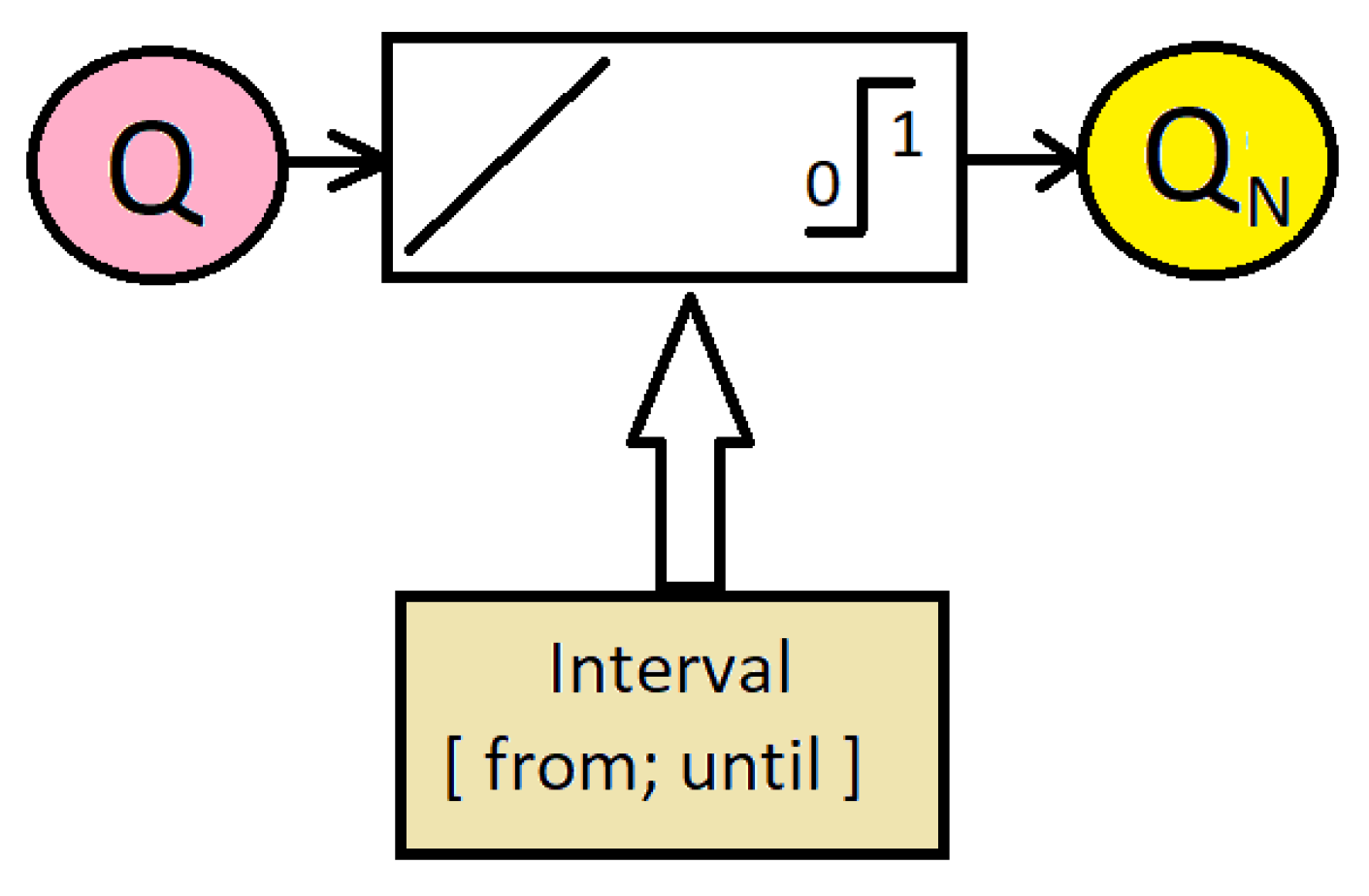
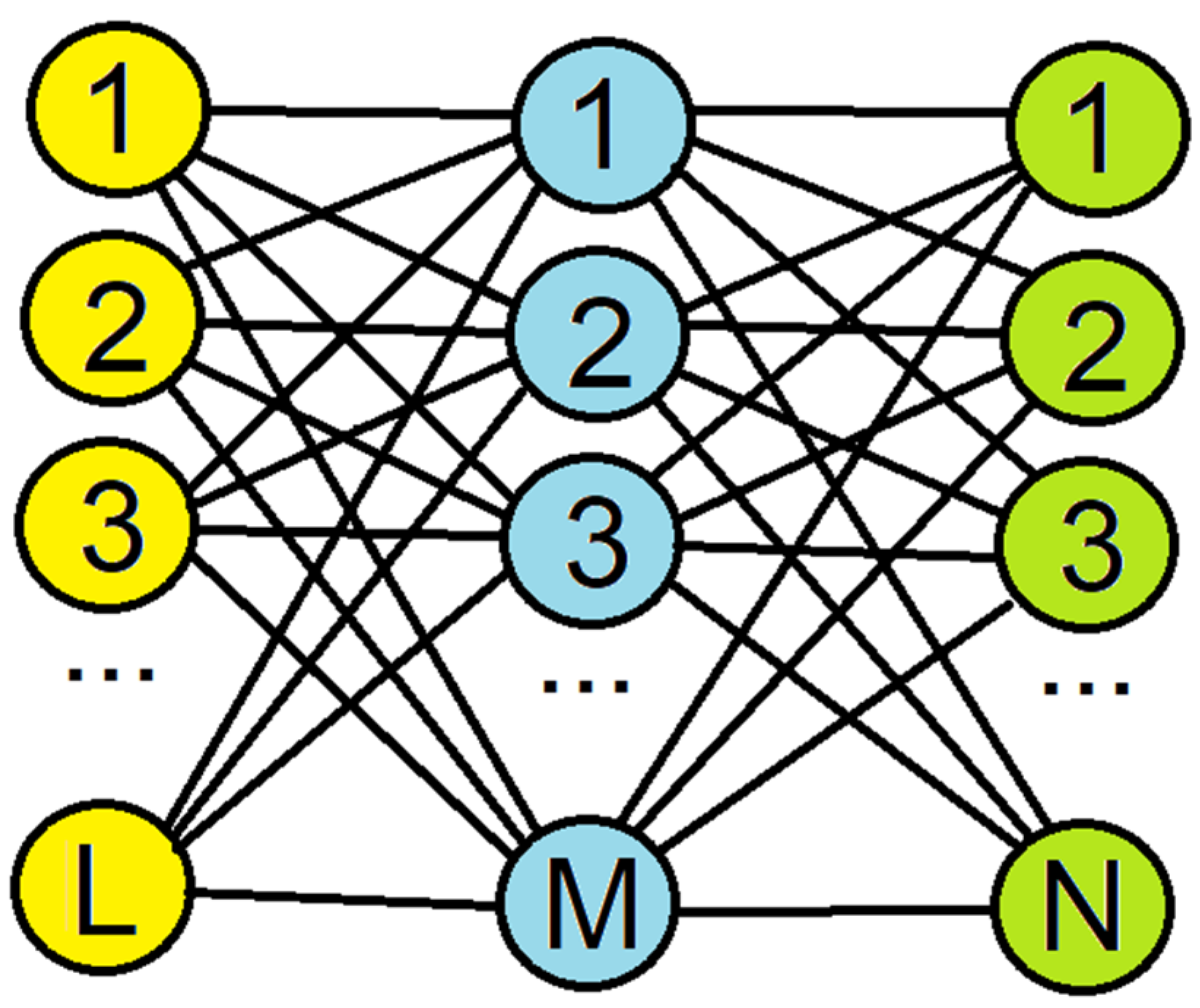
The advanced tool VALLUM01 [35] was constructed according to schemes presented in Figure 2 and Figure 3. Two different modules (a) for data conversion (from any real interval to fuzzy logic interval (0;1), forward and backward, see Figure 2) and (b) implementation of an ANN (see Figure 3) represent the main engines of the current project VALLUM01. All inputs are aggregated into the input layer, L = 12, all inputs are aggregated into the output layer N = 10. This ANN represents the implementation of one internal layer (called hidden), consisting of a requested number of perceptron M = (500;1000). Due to adjusting possibilities, bias was included in the hidden layer. The programmed package VALLUM01, which contains a graphical, user-friendly interface for input, output, and control, was created using the JAVA Eclipse framework. For ANNs, two typical classes from [36] were used: matrix and neural network. As an S-shaped function, a sigmoidal function was used:
σ ( x ) = 1 1 + e x

2.4. Organization of Data Input/Output

Real input data of the P01-P12 type (aggregated into the input layer, number of units L = 12) and real output data of the R00-R09 type (aggregated into the output layer, number of units N = 10), which express strong defined measurable physical quantities (see Table 3 and Table 4), were selected and approved for development. For an artificial neural network (ANN), input and output values must be presented in normalised form, which expresses the behaviour of fuzzy logic in the interval (0;1). Due to that, for all real values, the interval of distribution (XMIN; XMAX) was initially established (see Table 3 and Table 4). The module of data conversion recalculates the experimental input values Xi (i = 0 ; L ) and output values Yj (j  = 0 ; N ) to corresponding fuzzy logic values XXi and YYj in a forward or backward direction according to the formulas, respectively:
X X i = X i X M I N X M A X X M I N
X i = X M I N + X X i ( X M A X X M I N )

2.5. Test Campaign

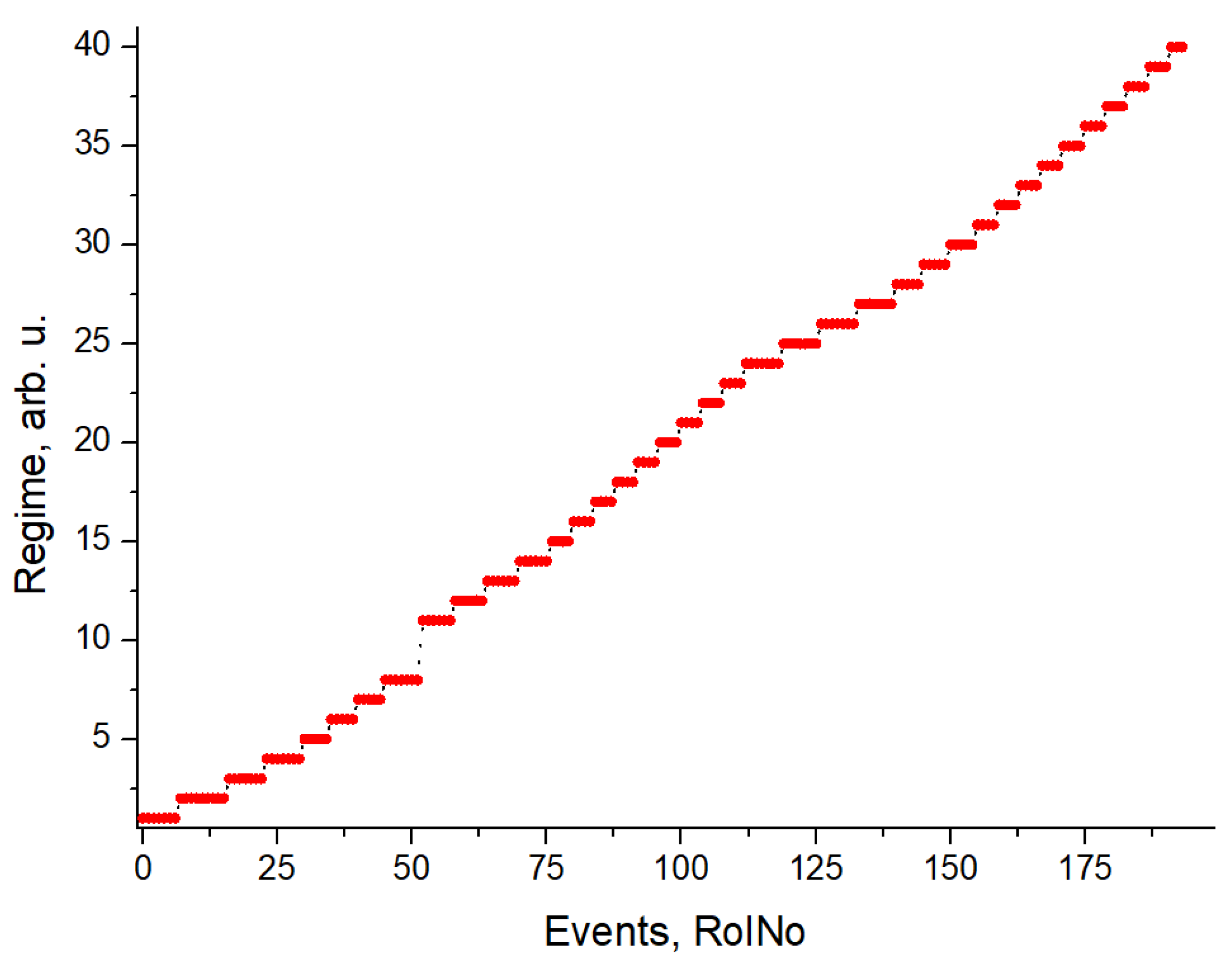
Figure 4 represents the distribution of experimental events (the current working state of the diesel engine) related to the different technical regimes (enumerated as 1…40). Experimental testing was carried out with the engine running at different speeds with varying loads, EGR, and SOI:
  • In the I stage (regimes 1–4, events, 1–30), the engine speed was set at 2000 rpm and the load was set at 30 Nm, 60 Nm, 90 Nm, and 120 Nm; the EGR was switched off, and the SOI (2–5 CAD bTDC) was controlled by the ECU.
  • In the II stage (regimes 5–8, events 31–52), the engine speed was set at 2500 rpm and the load was set at 30 Nm, 60 Nm, 90 Nm, and 120 Nm; the EGR was switched off, and the SOI (5–12 CAD bTDC) was controlled by the ECU.
  • In the III stage (regimes 11–14, events 53–76), the engine speed (2000 rpm) and load (60 Nm) were fixed, the EGR ratio was changed (0.05; 0.10; 0.15 and 0.20) using an EGR controller, and the SOI (3–4 CAD bTDC) was controlled by the ECU.
  • In the IV stage (regimes 15–23, 77–112), the engine speed (2000 rpm) and load (60 Nm) were fixed, EGR = 0.15 was set by the EGR controller, and fuel injection was changed by the SOI controller in the range of −3–15 CAD bTDC.
  • In the V stage (regimes 24–27, 113–140), the engine speed was set at 2500 rpm and the load was set at 30 Nm, 60 Nm, 90 Nm, and 120 Nm; the EGR ratio (0.35–0.05) and the SOI (5–10 CAD bTDC) were controlled by the ECU.
  • In the VI stage (regimes 28–31, 141–159), the engine speed was set at 2500 rpm and the load was set at 30 Nm, 60 Nm, 90 Nm, and 120 Nm; the EGR ratio (0.45–0.20) and the SOI (2–5 CAD bTDC) were controlled by the ECU.
  • In the VII stage (regimes 32–40, 160–195), the engine speed (2000 rpm) and load (60 Nm) were fixed, the controller set to EGR = 0.2, and the SOI controller varied the start of injection in the range of −3–15 CAD bTDC.
In these experimental studies, the engine was controlled both by the ECU’s default algorithm, by further modification of the control parameters, and by extending the field of operations.

3. Results

Simulations (training of ANN and output validation as a special case of prediction) were provided using a desktop computer, 11th Gen Intel(R) Core (TM) i5-11600K, 3.90 GHz, 32.0 GB RAM, and OS Windows 10 Pro. Programming package VALLUM01 (implementation of ANN in the regime of backpropagation, one hidden layer) was used for training and validation. The learning rate for training was established at 0.01 (without changes). Table 5 represents several simulation regimes for the usage and validation of ANN.
First, two training data sets (abc1.csv and bcd1.csv) consisting of P01–P12 and R00–R09 types were prepared. The set abc1.csv (size 194 events) represents pure experimental data without any filtering or mathematical development. Set abc1.csv consists of 40 subsets corresponding to the different technical regimes of diesel engines as presented in Figure 4. Set bcd1.csv (size 38 events) represents averaged data only (one averaged value per regime).
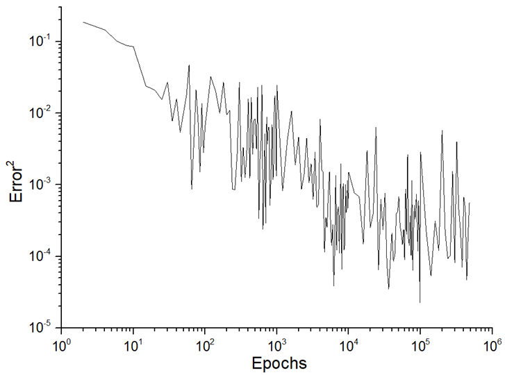
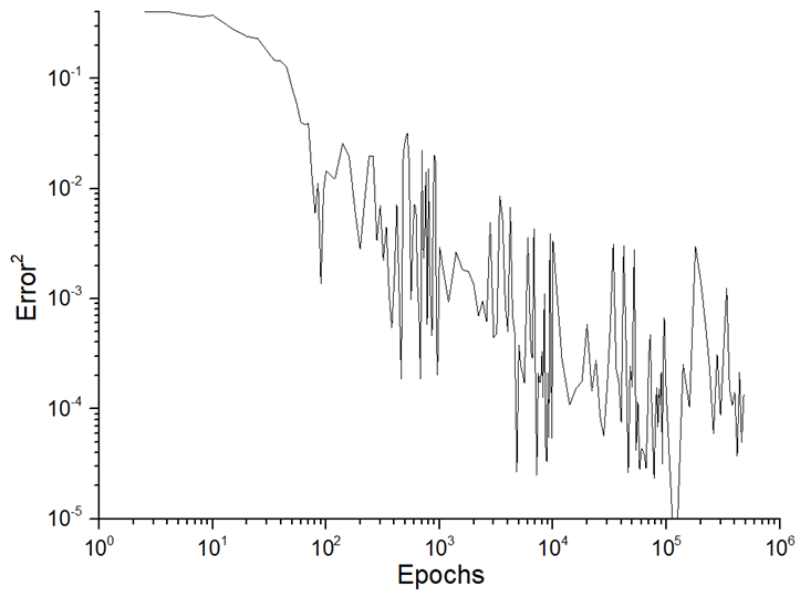
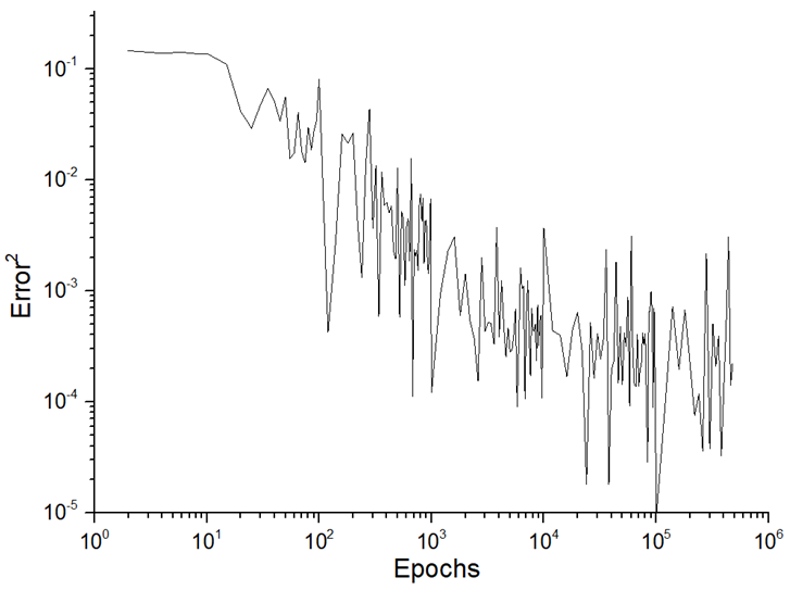
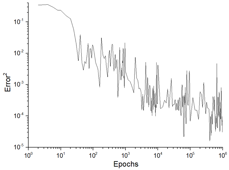
Second, six simulations (using different hidden layer, M = 500 ; 1000 ) for the validation of the data in the abc1.csv file were provided. Several different training routines T1–T6 were used by selecting the training data set (abc1.csv, real values of 194 events or, bcd1.csv, averaged values of 38 events, respectively), as well as by changing the number of training epochs (500,000; 1,000,000). Training was provided using the learning rate value of 0.01. Table 6 represents the distribution of the total network error (TNE), or error on the number of training epochs for different training regimes T1–T6: predefined by the number of training events and the number of perceptrons in hidden layers.
T N E 2 = 1 N i = 1 N X i c u r r e n t T a r g e t i 2
Table 5. The procedure of training and validation of ANNs. Input layer L = 12, output layer N = 10, amount of perceptron in the hidden layer M, learning rate 0.01.
ProjectOne Hidden LayerTrainingValidation
NameMRoutineFileEventsEpochsTNE2FileEvents
aaaa500T1abc1.csv194500,000Table 7, Table 8, Table 9, Table 10, Table 11 and Table 12abc1.csv194
bbbb500T2bcd1.csv38500,000Table 7, Table 8, Table 9, Table 10, Table 11 and Table 12abc1.csv194
cccc1000T3abc1.csv194500,000Table 7, Table 8, Table 9, Table 10, Table 11 and Table 12abc1.csv194
dddd1000T4bcd1.csv38500,000Table 7, Table 8, Table 9, Table 10, Table 11 and Table 12abc1.csv194
eeee1000T5abc1.csv1941,000,000Table 7, Table 8, Table 9, Table 10, Table 11 and Table 12abc1.csv194
ffff1000T6bcd1.csv381,000,000Table 7, Table 8, Table 9, Table 10, Table 11 and Table 12abc1.csv194
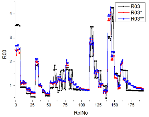
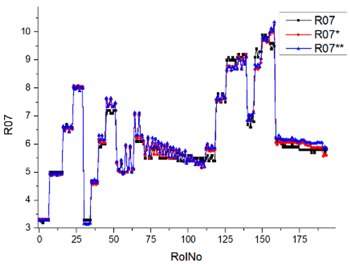
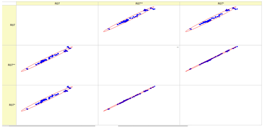
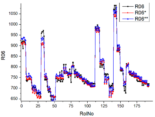
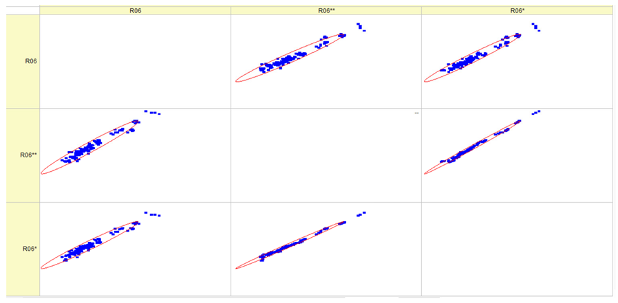
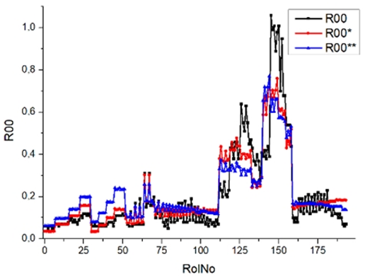
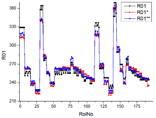
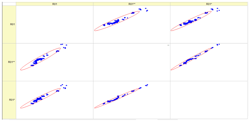
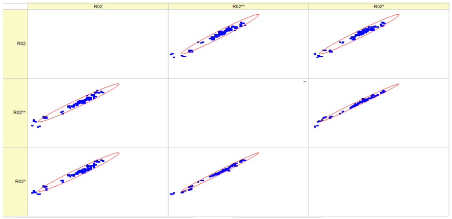
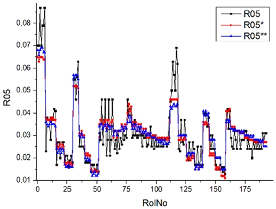
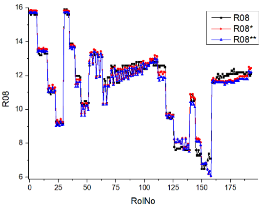
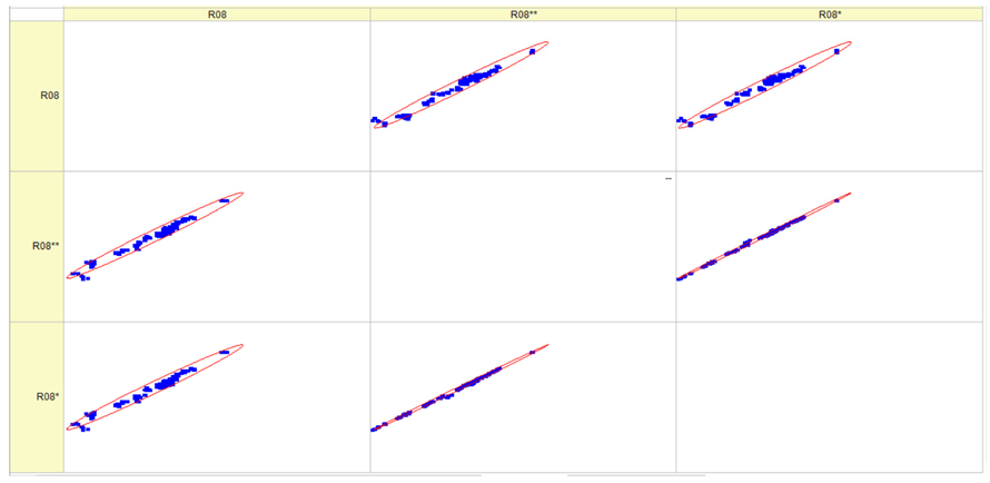
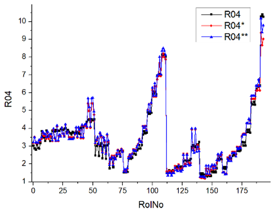
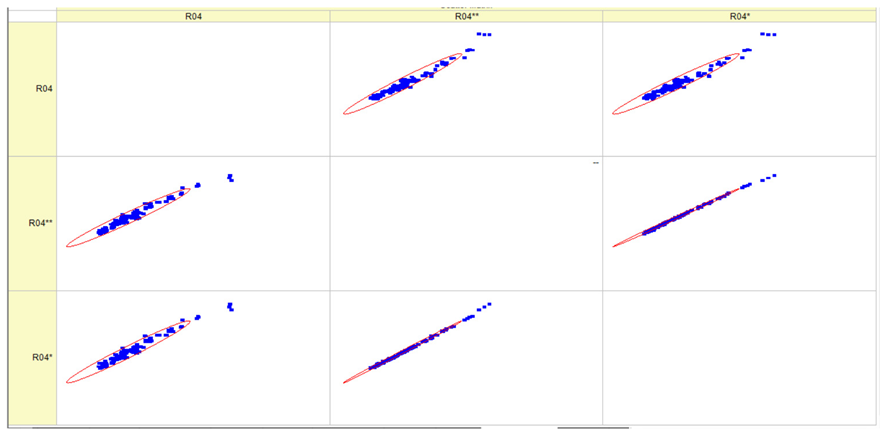
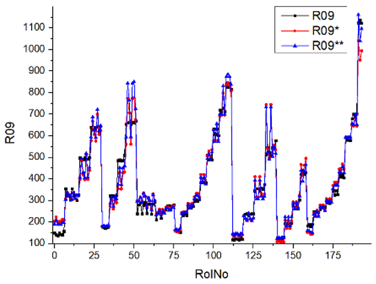
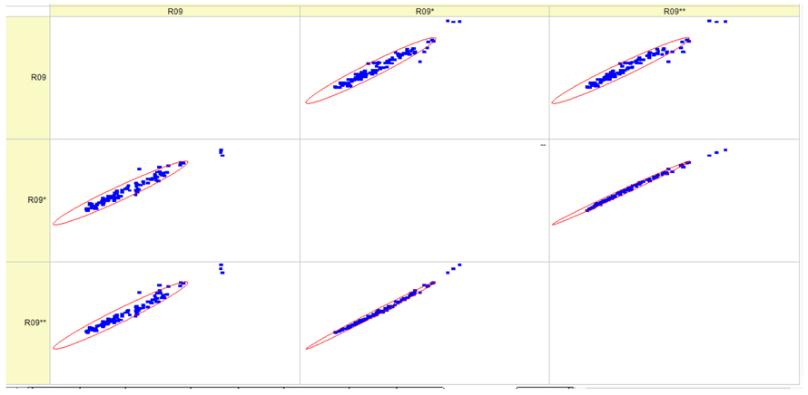
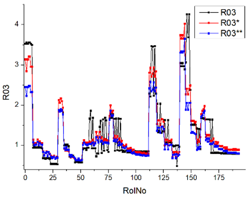
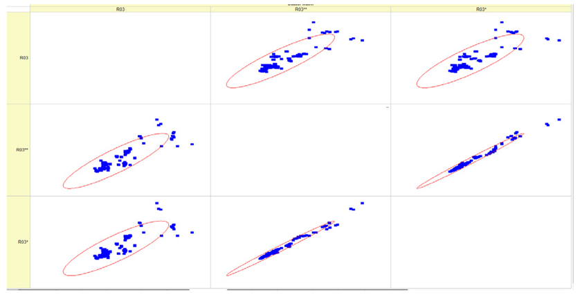
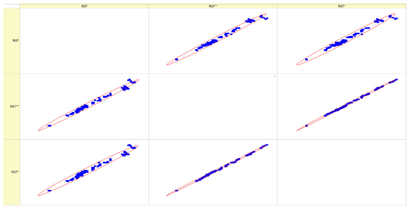
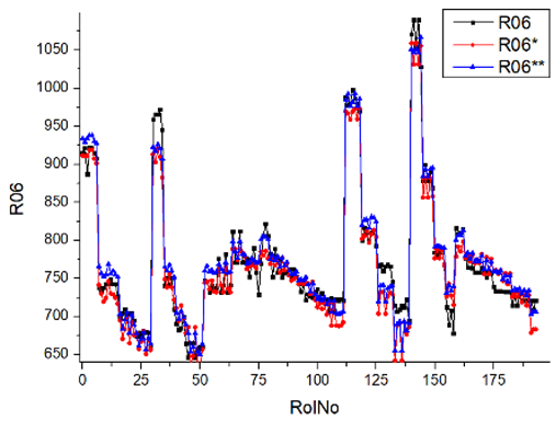
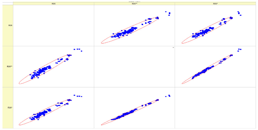
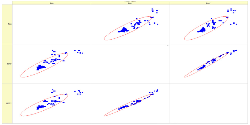
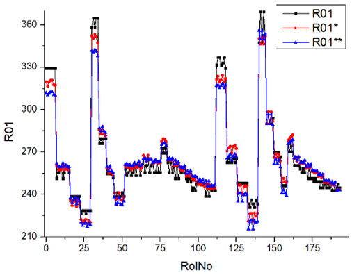
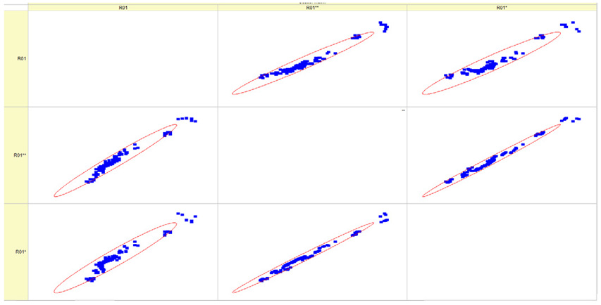
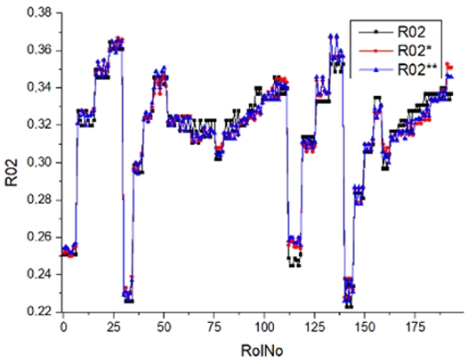
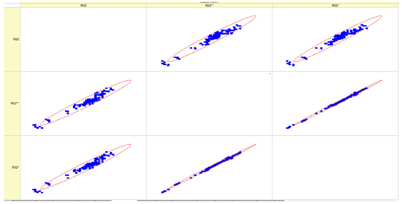
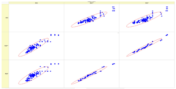
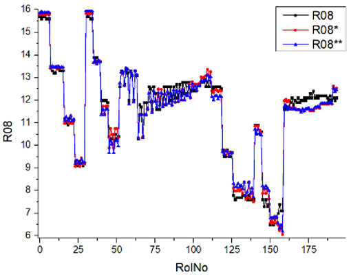
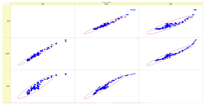
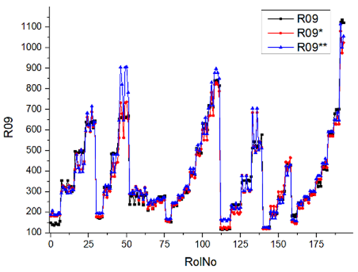
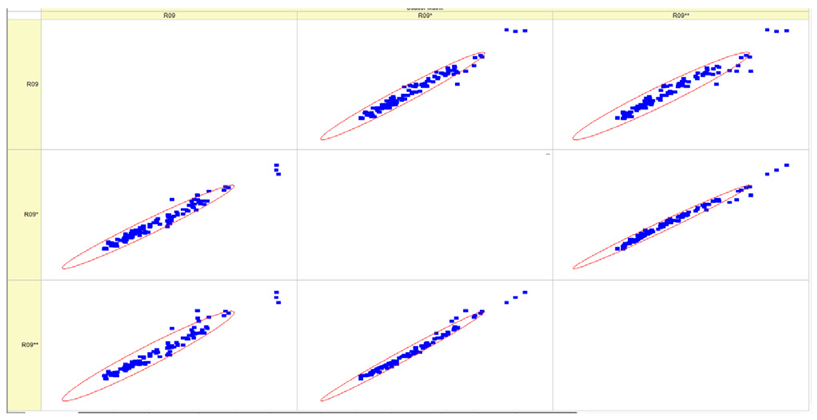
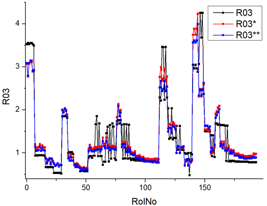
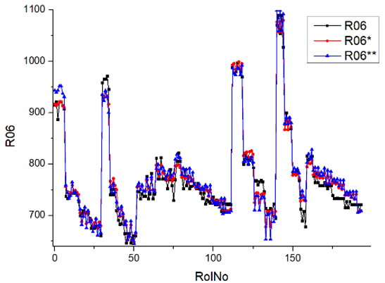
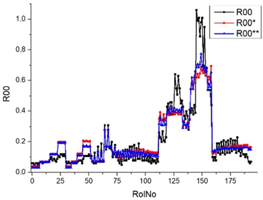
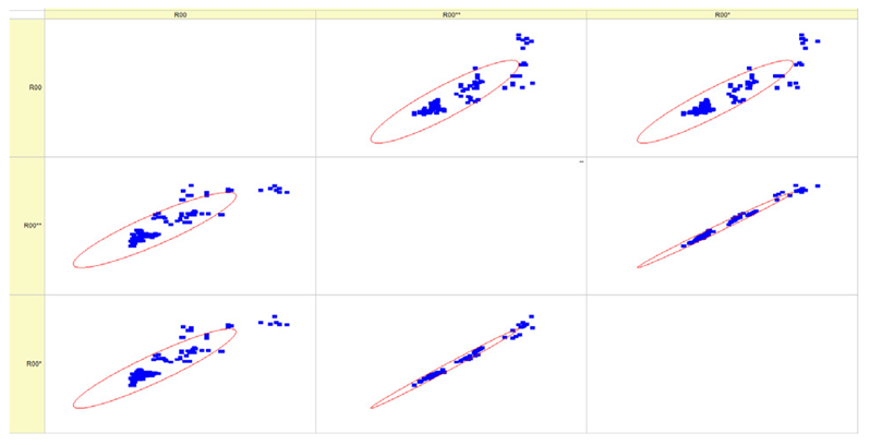
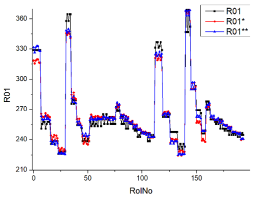
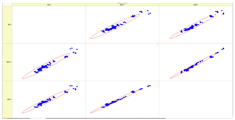
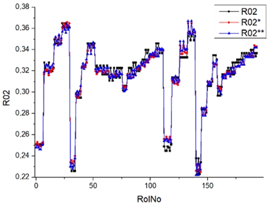
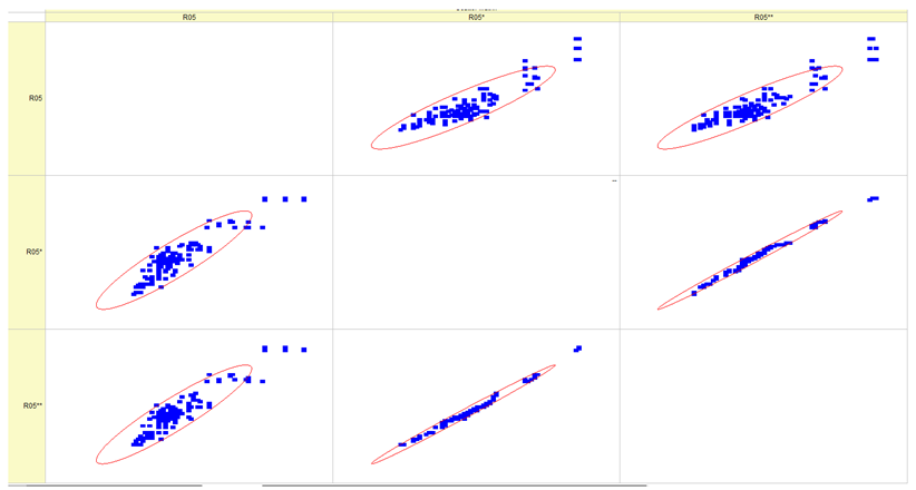
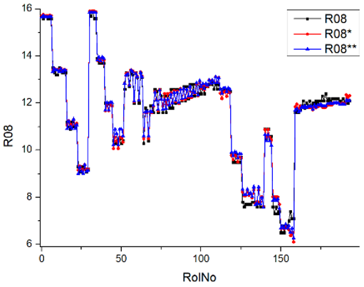
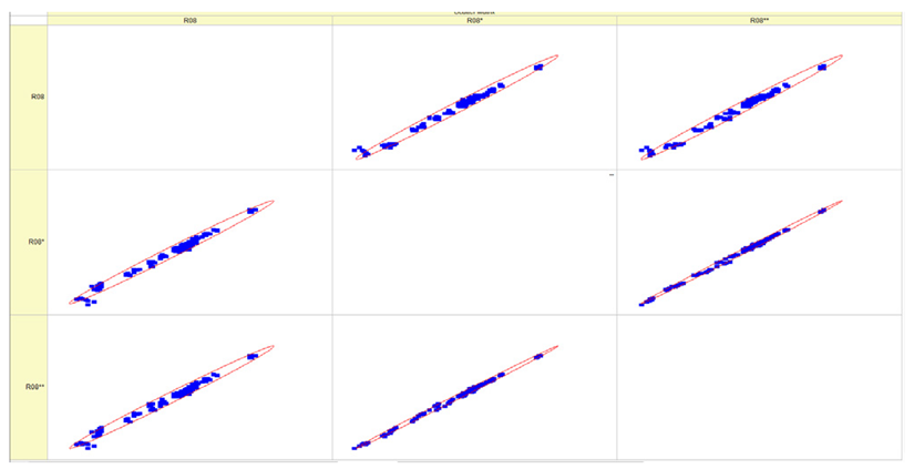
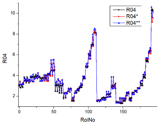
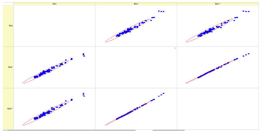
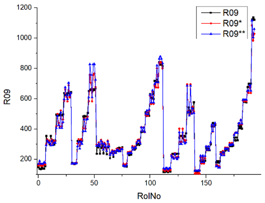
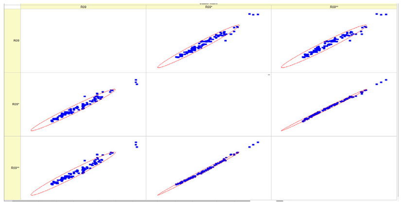
Table 7, Table 8, Table 9, Table 10, Table 11 and Table 12 represent the results of validation after training the ANN using different training regimes (T1–T6). Results are presented in the form of a triplet (R as the real experimental value, R* as predicted using the T1, T3, and T5 routine, and R** as predicted using the T2, T4, and T6 routine). Table 7, Table 9 and Table 11 represent distributions of predicted values R03, R07, R06, R00, and R01 and corresponding Pearson diagrams, and Table 8, Table 10 and Table 12 represent distributions of predicted values R02, R05, R08, R04, and R09 and corresponding Pearson diagrams. The smallest deviations between experimental and simulated values were obtained using training routines the T5 and T6 (see Table 5).

4. Discussion

The performance of ANNs is heavily dependent on the architecture and dynamic training mode. Three different stages were overcome to achieve a good result.
The first stage was related to the selection of interfaces. The output parameters (given in Table 4) are the measurement parameters that are appropriate to use for emission assessment. The number of output units for ANNs (N = 10) was established according to the experimental setup (R00…R09; see Table 4). For input parameters, two problems occur at the initial simulation. Firstly, we decided to use a significantly lower number of input parameters (L = 8). Parameters P00…P07 are traditional parameters that are suitable for the description of different power regimes of diesel engines (see Table 3). Unfortunately, the ANN learning process was unsuccessful. Then, we decided to increase the number of input units (L = 12) by adding several technical and physical parameters P08…P11 step-by-step, which allowed for receiving a satisfactory process of ANN learning. Secondly, the clusterization of input parameters needed realized using several technical and physical approaches. We decided to create the first input cluster according to the technical suggestions (P10, P03, P02, P11, and P01) and the second cluster according to the burning chemistry suggestions (P04, P05, P12, P06, P08, and P07). This assumption allows us to significantly improve the ANN learning process and avoid unpredictable increases in TNE.
The second stage pertains to the selection of the artificial neural network architecture. The feedforward method (information flow from the input layer through hidden layers to the output layer) was chosen due to the cause-and-effect relationship [37]. The possibility of using an ANN containing a single-hidden layer and multi-hidden layers was discovered and estimated. ANNs with double-hidden layers and triple-hidden layers are suitable for complex data containing hierarchical features. Generally, training an ANN with double- or triple-hidden layers is easier than with a single-hidden layer because fewer parameters require optimization. In our case, hierarchical-related data are absent. To decrease the wasting of computer resources (to decrease the training time), we decided to use the ANN containing a single-hidden layer due to the absence of multistep hierarchical behavior (see Table 3 and Table 4). The amount of perceptrons per hidden layer plays a crucial role in the training process. There is no general rule for the size of the hidden layer, but there are some empirical formulas. For example, Bekešienė et al. [27] presented some formulas for the expression of the size of the hidden layer (in our case, it would be M = 20…50). The decision was to increase M significantly per order and more by up to 500 and 1000. The regime of overfitting was exceeded at M = 2000. Due to that, the amount of perceptrons in the single-hidden layer must be in intervals (500; 1000). Bias was presented for adjusting purposes, but finally, we did not use this possibility to shift the argument of the action function sigmoid.
The third stage represents the training process. In the case of the single-hidden layer, we increased the starting number of training epochs (50,000) to 500,000 and 1,000,000, which allowed us to significantly improve the result. According to the distributions of TNE (see Figure 4), modes T5 and T6 must be named as satisfied. The quality of training could be established using the TNE parameter (see Equation (12)) or gradient distribution. We have used the TNE distribution, which allows us to assess the overtraining state and the unlearning state (both of which are indicators of incomplete training).
There were classifications for assessing the quality of ANN predictions as both a science and a kind of art. The quality of predictions is related to the training process, and the quantitative dynamical parameters of the training process determine further validation and prediction. The first approach to estimating the training process could be conducted using the TNE distribution (Figure 5). There was an exponential decrease in TNE as the number of epochs increased, which allowed the learning process to be called satisfied. In the interval from 500,000 to 1,000,000 epochs, the overtraining state was not distinguished (no significant increase in TNE distribution, more than two orders of magnitude or more). The second approach to estimating the training process is related to the existence of a plateau phase (i.e., saturation of the TNE distribution). In this case, this regime was distinguished after 100,000 epochs only (see Table 6).
Generally, it is impossible to evaluate which parameters have a less sensible result. The quality of training could be established using the TNE parameter (see Equation (12)) or gradient distribution. We have used TNE distribution, which allows us to assess the overtraining state (which is out of our interest). We have used several sets of input interfaces with different numbers of parameters (L = 7, 8, 10, and 12). Only one expanded set (P01–P12, L = 12; see Table 3) allows for a successful process of training. The possibility of removing several parameters from the expanded set (P01–P12, L = 12) was checked, but no significant training process was established.
The results in Table 7, Table 8, Table 9, Table 10, Table 11 and Table 12 can be used for a nondirected sensitivity analysis. This is possible when validation is shown along with Pearson distributions after training an ANN using different training regimes. The used ANN (feedforward ANN, two adjusted input, output interfaces, architecture of ANN (single-hidden layer, M = 500 and M = 1000) and dynamical regime—number of epochs 500,000 or 1,000,000)) allows to receive very high agreement between experimental and predicted results (R and R*, R and R**).
After evaluating the distributions of predicted values (Table 7, Table 8, Table 9, Table 10, Table 11 and Table 12), it is necessary to pay attention to the best prediction found for the first cluster: volumetric O2 concentration (R08), SNOx (R04), the volumetric concentration of NOx (R09), and SHC (R05). The third cluster contains SCO (R03), volumetric CO2 concentration (R07), and SCO2 (R06). The predictions of both clusters are in good agreement with the experimental ones.
The second cluster contains smoke (R00), brake specific fuel consumption (BSFC) (R01), and brake thermal efficiency (BTE) (R02). Especially for smoking, the predicted values are far from the experimental values. This large difference can be explained by measurement error (the effect of contaminant coupling in outcome tubes). A large deviation of smokiness (R00) between experimental and predicted values is essential when the V stage (regimes 24–27, 113–140) and the VI stage (regimes 28–31, 141–159) are distinguished. In all cases, extreme conditions (engine speed was set at 2500 rpm and the load was set at 30 Nm, 60 Nm, 90 Nm, and 120 N) have a bad correlation with the output parameter smokiness.
Figure 5 represents a comparison of different statistics: Pearson, Spearman, and Kendall.
Pearson, Spearman, and Kendall correlations were used to assess the magnitude and orientation of associations among variables. Figure 5 illustrates that the data dependencies exhibit a more linear pattern. As the number of epochs grows, the range of data quantiles reduces, resulting in a more condensed distribution. This is true for both the whole data package and the average data package, as demonstrated by the Pearson correlation. The Spearman correlation coefficient assists in comprehending the monotonic relationship of the data. It is evident that the data exhibited essentially identical variations while increasing the number of epochs and when analyzing the full and average data packets. The analyzed data is likely non-monotonic. Kendall’s correlation coefficient enables us to assess the degree of non-linearity in the data. Both Pearson and Kendall correlations demonstrate that the relationships in our dataset are linear in nature.
Commonly used statistical distributions show an exact and close-to-exact agreement between the experimental values and the expected ones. Pearson coefficient deviations are in the interval (3; 10%) (see Table 5). There were precise value predictions for the R00 (smokiness) distribution. The use of two training modes (500,000 and 1,000,000 epochs) and different ANN architectures (number of perceptrons 500 and 1000) cannot improve the result (RolNo110–130, 140–160, see Table 9, row R00 Smokiness). Perhaps the training data set for the R00 distribution (smokiness) is incomplete and requires partial experimental correlation. This hypothesis was made because only a few confirmed values deviated significantly from the experimental range. Evaluation of experimental regimes represents extreme engine operating conditions, and inaccurate predictions occur only at extreme regimes. Stage V (Modes 24–27, Rol No 110–130) was set at 2500 rpm, with a load of 90 Nm and 120 Nm. For stage VI (Modes 28–31, 140–159), the engine speed was set at 2500 rpm and the load was 60 Nm, 90 Nm, and 120 Nm. All series of experiments include the loads of 30, 60, 90, and 120 Nm. Two solutions to the presented problem could be formulated. Firstly, for extreme regimes, an incomplete set of input parameters must be supplemented by one or several parameters that allow the specified behavior of complex and complicated burning processes. Secondly, the experimental data set for training operations must be significantly increased, especially when using extreme regimes.
Other distributions (for example, R05 and SHC, see Table 12) show a close-to-satisfied agreement between the predicted values and the experimental ones. The R05 presents the experimental values in a chaotic manner, and the ANN prediction’s performance functions as a filter, averaging the weight.

5. Conclusions

  • The advanced tool VALLUM01 (with ANN implementation) containing a user-friendly interface for data input and output facilities was created, designed, and tested to provide simulations and predictions of exhausts in motor outcomes. A user-friendly input/output interface was created and used for solving the specific task of diesel motor efficiency using ANN. The set of input parameters (12) and output parameters (10) was estimated to be significant and sufficient for training, validation, and prediction. Intervals of values were recognized as suitable for fuzzification for input/output to ANN.
  • Training sessions for ANN (1,000,000 epochs, 1000 perceptrons in a single-hidden layer) could be titled as the most successful. For training, the use of averaged values instead of real experimental values is acceptable.
  • Following the development of a user-friendly input/output interface, the appropriateness of the input values for the artificial neural network (ANN) was verified (Table 3).
  • The first cluster, which includes volumetric O2 concentration, SNOx, and SHC, and the third cluster, which includes SCO, CO2 concentration, and SCO2, yielded the best predictions. However, the second cluster, including smoke, brake specific fuel consumption, and brake thermal efficiency, showed significant deviations from experimental values, mainly due to measurement error and extreme conditions.

Author Contributions

Conceptualization, J.M., A.R. and A.G.; methodology, J.M., A.R. and A.G.; software, J.M. and A.G.; validation, J.M., A.R. and A.G.; formal analysis, J.M. and A.G.; investigation, J.M., A.R. and A.G.; resources, J.M., A.R. and A.G.; data curation, J.M., A.R. and A.G.; writing—original draft preparation, J.M., A.R. and A.G.; writing—review and editing, J.M., A.R. and A.G.; visualization, J.M., A.R. and A.G.; supervision, J.M.; project administration, J.M.; funding acquisition, J.M. and A.R. All authors have read and agreed to the published version of the manuscript.

Funding

This research received no external funding.

Data Availability Statement

Data could be provided according to request.

Conflicts of Interest

The authors declare no conflicts of interest.

Abbreviations

λThe excess air ratio
AIArtificial intelligence
ANNArtificial neural networks
BMEPBrake mean effective pressure
BTEBrake thermal efficiency
BSFCBrake specific fuel consumption
CO2Carbon dioxide
COCarbon monoxide
D100Pure fossil diesel fuel
ECUEngine control unit
EGRExhaust gas recirculation
HCHydrocarbons
HVO100Hydrotreated Vegetable Oil
l0Stoichiometric air to fuel ratio
LHVLower heating value
MLMachine Learning
MLPMultilayer perceptron
MLPNNMultilayer perceptron neural network
NOxNitrogen oxides
RSMResponse surface methodology
SCO2Recalculated CO2 value
SCORecalculated CO value
SHCRecalculated HC value
SOSmoke opacity
SOIStart of injection
SNOxRecalculated NOx value
TNETotal network error
H2OWater

References

  1. Ulbrich, D.; Selech, J.; Kowalczyk, J.; Jóźwiak, J.; Durczak, K.; Gil, L.; Pieniak, D.; Paczkowska, M.; Przystupa, K. Reliability Analysis for Unrepairable Automotive Components. Materials 2021, 14, 7014. [Google Scholar] [CrossRef]
  2. Oulmelk, A.; Srati, M.; Afraites, L.; Hadri, A. An Artificial Neural Network Approach to Identify the Parameter in a Nonlinear Subdiffusion Model. Commun. Nonlinear Sci. Numer. Simul. 2023, 125, 107413. [Google Scholar] [CrossRef]
  3. Borucka, A.; Kozłowski, E.; Antosz, K.; Parczewski, R. A New Approach to Production Process Capability Assessment for Non-Normal Data. Appl. Sci. 2023, 13, 6721. [Google Scholar] [CrossRef]
  4. Žvirblis, T.; Hunicz, J.; Matijošius, J.; Rimkus, A.; Kilikevičius, A.; Gęca, M. Improving Diesel Engine Reliability Using an Optimal Prognostic Model to Predict Diesel Engine Emissions and Performance Using Pure Diesel and Hydrogenated Vegetable Oil. Eksploat. I Niezawodn.–Maint. Reliab. 2023, 25, 174358. [Google Scholar] [CrossRef]
  5. Sindhu, T.N.; Çolak, A.B.; Lone, S.A.; Shafiq, A.; Abushal, T.A. A Decreasing Failure Rate Model with a Novel Approach to Enhance the Artificial Neural Network’s Structure for Engineering and Disease Data Analysis. Tribol. Int. 2023, 192, 109231. [Google Scholar] [CrossRef]
  6. Alam, M.S.; Deb, J.B.; Amin, A.A.; Chowdhury, S. An Artificial Neural Network for Predicting Air Traffic Demand Based on Socio-Economic Parameters. Decis. Anal. J. 2024, 10, 100382. [Google Scholar] [CrossRef]
  7. AlAlaween, W.H.; Mahfouf, M.; Omar, C.; Al-Asady, R.B.; Monaco, D.; Salman, A.D. Serial Artificial Neural Networks Characterized by Gaussian Mixture for the Modelling of the Consigma25 Continuous Manufacturing Line. Powder Technol. 2024, 434, 119296. [Google Scholar] [CrossRef]
  8. Soori, M.; Arezoo, B.; Dastres, R. Artificial Neural Networks in Supply Chain Management, a Review. J. Econ. Technol. 2023, 1, 179–196. [Google Scholar] [CrossRef]
  9. Adedeji, B.P. Electric Vehicles Survey and a Multifunctional Artificial Neural Network for Predicting Energy Consumption in All-Electric Vehicles. Results Eng. 2023, 19, 101283. [Google Scholar] [CrossRef]
  10. Sahin, G.; Isik, G.; van Sark, W.G.J.H.M. Predictive Modeling of PV Solar Power Plant Efficiency Considering Weather Conditions: A Comparative Analysis of Artificial Neural Networks and Multiple Linear Regression. Energy Rep. 2023, 10, 2837–2849. [Google Scholar] [CrossRef]
  11. Zurada, J.M. Introduction to Artificial Neural Systems; West: St. Paul, MN, USA, 1992; ISBN 978-0-314-93391-1. [Google Scholar]
  12. Rabunal, J.R.; Dorado, J. (Eds.) Artificial Neural Networks in Real-Life Applications; Idea Group Pub: Hershey, PA, USA, 2006; ISBN 978-1-59140-902-1. [Google Scholar]
  13. Goodfellow, I.; Bengio, Y.; Courville, A. Deep Learning. Available online: https://www.deeplearningbook.org/ (accessed on 31 December 2023).
  14. Torres Sospedra, J. Ensembles of Artificial Neural Networks: Analysis and Development of Design Methods; Universitat Jaume I. Departament d’Enginyeria i Ciència dels Computadors: Castellon, Spain, 2011. [Google Scholar]
  15. Lou, C. Artificial Neural Networks: Their Training Process and Applications; Department of Mathematics Whitman College: Walla Walla, WA, USA, 2019. [Google Scholar]
  16. Li, R.; Herreros, J.M.; Tsolakis, A.; Yang, W. Integrated Machine Learning-Quantitative Structure Property Relationship (ML-QSPR) and Chemical Kinetics for High Throughput Fuel Screening toward Internal Combustion Engine. Fuel 2022, 307, 121908. [Google Scholar] [CrossRef]
  17. Ahmad, I.; Sana, A.; Kano, M.; Cheema, I.I.; Menezes, B.C.; Shahzad, J.; Ullah, Z.; Khan, M.; Habib, A. Machine Learning Applications in Biofuels’ Life Cycle: Soil, Feedstock, Production, Consumption, and Emissions. Energies 2021, 14, 5072. [Google Scholar] [CrossRef]
  18. Usman, M.; Jamil, M.K.; Ashraf, W.M.; Saqib, S.; Ahmad, T.; Fouad, Y.; Raza, H.; Ashfaq, U.; Pervaiz, A. AI-Driven Optimization of Ethanol-Powered Internal Combustion Engines in Alignment with Multiple SDGs: A Sustainable Energy Transition. Energy Convers. Manag. X 2023, 20, 100438. [Google Scholar] [CrossRef]
  19. Deng; Jiamei; Stobart; Richard; Basti, M. The Applications of Artificial Neural Networks to Engines. In Artificial Neural Networks-Industrial and Control Engineering Applications; Suzuki, K., Ed.; InTech: Vienna, Austria, 2011; ISBN 978-953-307-220-3. [Google Scholar]
  20. Xing, Y.; Zheng, Z.; Sun, Y.; Agha Alikhani, M. A Review on Machine Learning Application in Biodiesel Production Studies. Int. J. Chem. Eng. 2021, 2021, 2154258. [Google Scholar] [CrossRef]
  21. Aliramezani, M.; Koch, C.R.; Shahbakhti, M. Modeling, Diagnostics, Optimization, and Control of Internal Combustion Engines via Modern Machine Learning Techniques: A Review and Future Directions. Prog. Energy Combust. Sci. 2022, 88, 100967. [Google Scholar] [CrossRef]
  22. Zhang, L.; Zhu, G.; Chao, Y.; Chen, L.; Ghanbari, A. Simultaneous Prediction of CO2, CO, and NOx Emissions of Biodiesel-Hydrogen Blend Combustion in Compression Ignition Engines by Supervised Machine Learning Tools. Energy 2023, 282, 128972. [Google Scholar] [CrossRef]
  23. Khac, H.N.; Modabberian, A.; Zenger, K.; Niskanen, K.; West, A.; Zhang, Y.; Silvola, E.; Lendormy, E.; Storm, X.; Mikulski, M. Machine Learning Methods for Emissions Prediction in Combustion Engines with Multiple Cylinders. IFAC-PapersOnLine 2023, 56, 3072–3078. [Google Scholar] [CrossRef]
  24. Venkatesh, S.N.; V, S.; Thangavel, V.; Balaji P, A.; Vijayaragavan, M.; Subramanian, B.; Josephin JS, F.; Varuvel, E.G. Efficacy of Machine Learning Algorithms in Estimating Emissions in a Dual Fuel Compression Ignition Engine Operating on Hydrogen and Diesel. Int. J. Hydrogen Energy 2023, 48, 39599–39611. [Google Scholar] [CrossRef]
  25. Lionus Leo, G.M.; Jayabal, R.; Srinivasan, D.; Chrispin Das, M.; Ganesh, M.; Gavaskar, T. Predicting the Performance and Emissions of an HCCI-DI Engine Powered by Waste Cooking Oil Biodiesel with Al2O3 and FeCl3 Nano Additives and Gasoline Injection—A Random Forest Machine Learning Approach. Fuel 2024, 357, 129914. [Google Scholar] [CrossRef]
  26. Williams, Z.; Moiz, A.; Cung, K.; Smith, M.; Briggs, T.; Bitsis, C.; Miwa, J. Generation of Rate-of-Injection (ROI) Profile for Computational Fluid Dynamics (CFD) Model of Internal Combustion Engine (ICE) Using Machine Learning. Energy AI 2022, 8, 100148. [Google Scholar] [CrossRef]
  27. Bekesiene, S.; Smaliukiene, R.; Vaicaitiene, R. Using Artificial Neural Networks in Predicting the Level of Stress among Military Conscripts. Mathematics 2021, 9, 626. [Google Scholar] [CrossRef]
  28. Jovanović, N.; Vasović, B.; Jovanović, Z.; Cvjetković, M. Neural Network Implementation in Java. Bizinfo 2020, 11, 19–30. [Google Scholar] [CrossRef]
  29. Godwin, D.J.; Varuvel, E.G.; Martin, M.L.J. Prediction of Combustion, Performance, and Emission Parameters of Ethanol Powered Spark Ignition Engine Using Ensemble Least Squares Boosting Machine Learning Algorithms. J. Clean. Prod. 2023, 421, 138401. [Google Scholar] [CrossRef]
  30. Valeika, G.; Matijošius, J.; Górski, K.; Rimkus, A.; Smigins, R. A Study of Energy and Environmental Parameters of a Diesel Engine Running on Hydrogenated Vegetable Oil (HVO) with Addition of Biobutanol and Castor Oil. Energies 2021, 14, 3939. [Google Scholar] [CrossRef]
  31. Rimkus, A.; Žaglinskis, J.; Stravinskas, S.; Rapalis, P.; Matijošius, J.; Bereczky, Á. Research on the Combustion, Energy and Emission Parameters of Various Concentration Blends of Hydrotreated Vegetable Oil Biofuel and Diesel Fuel in a Compression-Ignition Engine. Energies 2019, 12, 2978. [Google Scholar] [CrossRef]
  32. Shepel, O.; Matijošius, J.; Rimkus, A.; Duda, K.; Mikulski, M. Research of Parameters of a Compression Ignition Engine Using Various Fuel Mixtures of Hydrotreated Vegetable Oil (HVO) and Fatty Acid Esters (FAE). Energies 2021, 14, 3077. [Google Scholar] [CrossRef]
  33. Ross-Tech: Home. Available online: https://www.ross-tech.com/index.php (accessed on 31 December 2023).
  34. Heywood, J.B. Internal Combustion Engine Fundamentals, 2nd ed.; McGraw-Hill Education: New York, NY, USA, 2018; ISBN 978-1-260-11610-6. [Google Scholar]
  35. Gruodis, A. VALLUM01. Advanced Tool for Implementation of Artificial Neural Network Containing Tabular Interface for Input/Output 2023. Available online: https://github.com/solo51/VALLUM (accessed on 31 December 2023).
  36. Sonawane, S. Understanding and Implementing Neural Networks in Java from Scratch. Available online: https://towardsdatascience.com/understanding-and-implementing-neural-networks-in-java-from-scratch-61421bb6352c (accessed on 31 December 2023).
  37. Gruodis, A. Realizations of the Artificial Neural Network for Process Modeling. Overview of Current Implementations. Appl. Bus. Issues Solut. 2023, 2, 22–27. [Google Scholar] [CrossRef]
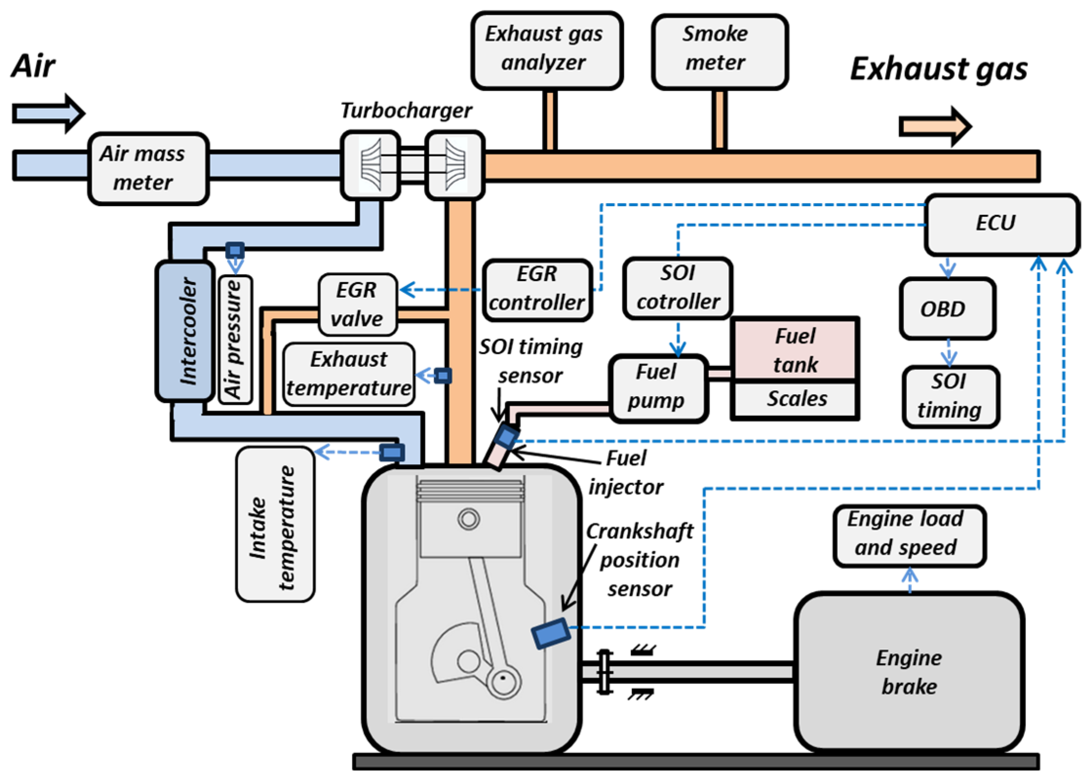
Figure 1. Scheme of engine test equipment.
Machines 12 00279 g001
Figure 2. Advanced tool VALLUM01: scheme of data input/output.
Machines 12 00279 g002
Figure 3. Scheme of an artificial neural network (ANN): input layer, number of units L = 12, single-hidden layer, number of perceptron M = (500;1000), output layer, number of units N = 10.
Machines 12 00279 g003
Figure 4. Experimental events (0…196) related to the different technical regimes (1…40) of diesel engines.
Machines 12 00279 g004
Figure 5. Comparison of different statistics: Pearson, Spearman, and Kendall.
Machines 12 00279 g005
Table 1. Main parameters of a 1.9 TDI compression ignition. Adapted according to [30].
ParameterUnitsValue
Displacement, VHdm31.896
Number of cylinders, i-4/OHC
Number of engine strokes, τ-4
Compression ratio-19.5
PowerkW66 (4000 rpm)
TorqueNm180 (2000–2500 rpm)
Boremm79.5
Strokemm95.5
Fuel injection-Direct injection (single)
Nozzle type and holder assembly-Hole-type, two spring
Nozzle opening pressurebar190
Table 2. Main properties of the fuels tested. Adapted according to [32].
PropertiesUnitsHVO100EN 15940D100EN 590
Density at 15 °Cg/mL0.7820.765–0.8000.8380.820–0.845
Kinematic viscosity at 40 °CcSt2.8762.000–4.5002.94012.000–4.500
Cold filter plugging point°C–44≤+5… ≤–44 *–22≤+5… ≤–44 *
Pour point°C<–50≤–10 *… ≤–34 *–39≤–10 *… ≤–34 *
Flash point°C65.0> 55.074.8>55.0
Water content% V/V0.0021≤0.0200.0028≤0.020
Lubricityµm344≤460406≤460
Cetane number-74.3≥70~53≥51.0
Elemental composition (H)%15.62-13.31-
Elemental composition (C)%84.38-86.69-
C/H ratio 5.40-6.51-
Stoichiometric air to fuel ratio ( l 0 )kg air/1 kg fuel15.10-14.50-
Lower heating value (LHV)MJ/kg43.63≈4442.83≈43
* Severe winter and arctic grades.
Table 3. Experimental parameters of diesel engine used for an ANN as the input parameters.
IndexAbbr.ParameterUnitsInterval
XMINXMAX
0P10 The   excess   air   ratio   ( λ ) -1.010.0
1P03 Brake   mean   effective   pressure   ( B M E P ) MPa0.01.2
2P02EGR ratio-0.00.5
3P11Start of injection (SOI)CA bTDC−3.018.0
4P09Cetane number-5.085.0
5P01Engine speed (n)rpm800.04000.0
6P04Volume fraction of HVO100%0.0100.0
7P05Volume fraction of D100%0.0100.0
8P12C/H ratio-5.07.0
9P06 Stoichiometric   air   to   fuel   ratio   ( l 0 )1 kg of air/1 kg of fuel10.020.0
10P08Lower heating value (LHV)MJ·kg−118.060.0
11P07Densitykg·m−3600.0900.0
Table 4. Experimental parameters of diesel engine used for ANN as the output parameters.
IndexAbbr.ParameterUnitsInterval
YMINYMAX
0R03SCOg·kWh−10.510.0
1R07Volumetric CO2 concentration %0.115.0
2R06SCO2g·kWh−1100.02000.0
3R00Smokiness m−10.001100.0
4R01Brake specific fuel consumption (BSFC)g·kWh−1150.03000.0
5R02Brake thermal efficiency (BTE)-0.010.5
6R05SHCg·kWh−10.012.0
7R08Volumetric O2 concentration%0.520.0
8R04SNOxg·kWh−10.120.0
9R09Volumetric NOx concentrationppm10.010,000.0
Table 6. Distribution of the TNE2 on the number of training epochs for different training regimes T1–T6: predefined by number of training events and number of hidden layers.
Hidden Layer
EpochsEventsM = 500M = 1000
500,000194Machines 12 00279 i001Machines 12 00279 i002
500,00038Machines 12 00279 i003Machines 12 00279 i004
1,000,000194xMachines 12 00279 i005
1,000,00038xMachines 12 00279 i006
Table 7. Results of validation after training of ANNs (one hidden layer, M = 500 ). Distributions of predicted values R03, R07, R06, R00, and R01 and corresponding Pearson diagrams. Two different training routines T1 and T2 were used (see Table 5). Number of training epochs: 500,000. Distributions of values: R as real experimental value, R* as predicted using T1 routine, and R** as predicted using T2 routine). Number of events for validation 194.
AbbrParameterDistributions of Predicted ValuePearson
R03SCO,
g·kWh−1
Machines 12 00279 i007Machines 12 00279 i008
R07Volumetric CO2 concentration, %Machines 12 00279 i009Machines 12 00279 i010
R06SCO2,
g·kWh−1
Machines 12 00279 i011Machines 12 00279 i012
R00Smokiness,
m−1
Machines 12 00279 i013Machines 12 00279 i014
R01Brake specific fuel consumption (BSFC),
g·kWh−1
Machines 12 00279 i015Machines 12 00279 i016
Table 8. Results of validation after training of ANN (one hidden layer, M = 500). Distributions of predicted values R02, R05, R08, R04, and R09 and corresponding Pearson diagrams. Two different training routines T1 and T2 were used (see Table 5). Number of training epochs: 500,000. Distributions of values: R as real experimental value, R* as predicted using the T1 routine, and R** as predicted using the T2 routine. Number of events for validation 194.
AbbrParameterDistribution of Predicted ValuePearson
R02Brake thermal efficiency (BTE)Machines 12 00279 i017Machines 12 00279 i018
R05SHC,
g·kWh−1
Machines 12 00279 i019Machines 12 00279 i020
R08Volumetric O2 concentration, %Machines 12 00279 i021Machines 12 00279 i022
R04SNOx,
g·kWh−1
Machines 12 00279 i023Machines 12 00279 i024
R09Volumetric NOx concentration, ppmMachines 12 00279 i025Machines 12 00279 i026
Table 9. Results of validation after training of ANNs (one hidden layer, M =   1000 ). Distributions of predicted values R03, R07, R06, R00, and R01 and corresponding Pearson diagrams. Two different training routines T3 and T4 were used (see Table 5). Number of training epochs 500,000. Distributions of values: R as real experimental value, R* as predicted using the T3 routine, and R** as predicted using T4 routine. Number of events for validation 194.
AbbrParameterDistributions of Predicted ValuePearson
R03SCO,
g·kWh−1
Machines 12 00279 i027Machines 12 00279 i028
R07Volumetric CO2 concentration, %Machines 12 00279 i029Machines 12 00279 i030
R06SCO2,
g·kWh−1
Machines 12 00279 i031Machines 12 00279 i032
R00Smokiness,
m−1
Machines 12 00279 i033Machines 12 00279 i034
R01Brake specific fuel consumption (BSFC),
g·kWh−1
Machines 12 00279 i035Machines 12 00279 i036
Table 10. Results of validation after training of ANNs (one hidden layer, M =   1000 ). Distributions of predicted values R02, R05, R08, R04, and R09 and corresponding Pearson diagrams. Two different training routines T3 and T4 were used (see Table 5). Number of training epochs: 500,000. Distributions of values: R as real experimental value, R* as predicted using the T3 routine, and R** as predicted using the T4 routine. Number of events for validation 194.
AbbrParameterDistribution of Predicted ValuePearson
R02Brake thermal efficiency (BTE)Machines 12 00279 i037Machines 12 00279 i038
R05SHC,
g·kWh−1
Machines 12 00279 i039Machines 12 00279 i040
R08Volumetric O2 concentration, %Machines 12 00279 i041Machines 12 00279 i042
R04SNOx,
g·kWh−1
Machines 12 00279 i043Machines 12 00279 i044
R09Volumetric NOx concentration, ppmMachines 12 00279 i045Machines 12 00279 i046
Table 11. Results of validation after training of ANNs (one hidden layer, M =   1000 ). Distributions of predicted values R03, R07, R06, R00, and R01 and corresponding Pearson diagrams. Two different training routines T5 and T6 were used (see Table 5). Number of training epochs: 1,000,000. Distributions of values: R as real experimental value, R* as predicted using the T5 routine, and R** as predicted using the T6 routine. Number of events for validation 194.
AbbrParameterDistributions of Predicted ValuePearson
R03SCO,
g·kWh−1
Machines 12 00279 i047Machines 12 00279 i048
R07Volumetric CO2 concentration, %Machines 12 00279 i049Machines 12 00279 i050
R06SCO2,
g·kWh−1
Machines 12 00279 i051Machines 12 00279 i052
R00Smokiness,
m−1
Machines 12 00279 i053Machines 12 00279 i054
R01Brake specific fuel consumption (BSFC),
g·kWh−1
Machines 12 00279 i055Machines 12 00279 i056
Table 12. Results of validation after training of ANNs (one hidden layer, M =   1000 ). Distributions of predicted values R02, R05, R08, R04, and R09 and corresponding Pearson diagrams. Two different training routines T5 and T6 were used (see Table 5). Number of training epochs: 1,000,000. Distributions of values: R as real experimental value, R* as predicted using the T5 routine, and R** as predicted using the T6 routine. Number of events for validation 194.
AbbrParameterDistribution of Predicted ValuePearson
R02Brake thermal efficiency (BTE)Machines 12 00279 i057Machines 12 00279 i058
R05SHC,
g·kWh−1
Machines 12 00279 i059Machines 12 00279 i060
R08Volumetric O2 concentration, %Machines 12 00279 i061Machines 12 00279 i062
R04SNOx,
g·kWh−1
Machines 12 00279 i063Machines 12 00279 i064
R09Volumetric NOx concentration, ppmMachines 12 00279 i065Machines 12 00279 i066
Disclaimer/Publisher’s Note: The statements, opinions and data contained in all publications are solely those of the individual author(s) and contributor(s) and not of MDPI and/or the editor(s). MDPI and/or the editor(s) disclaim responsibility for any injury to people or property resulting from any ideas, methods, instructions or products referred to in the content.