Magnetic Field Analysis and Thrust Verification of Solenoid Actuator Based on Subdomain Method

Abstract

In view of the problem that the output thrust of the solenoid actuator is affected by various factors and is difficult to calculate in actual working conditions, this paper proposes a semi-analytical model constructed by magnetic field subdomain method with internal and external boundary conditions in a cylindrical coordinate system for calculation, and the general solution equations of magnetic vector potential for each subdomain are derived and solved by MATLAB. Taking a push–pull electromagnet as an example, the finite element simulation and experimental comparative analysis are carried out. The correctness and applicable conditions of the subdomain method are illustrated by comparing the gradient plot of magnetic vector potential, inductance curve and electromagnetic force. It is shown that the results calculated by the subdomain method are very close to the finite element method when the magnetic saturation problem is neglected. However, when the nonlinearity of core permeability is considered, the magnetic saturation gradually deepens with the increase in current, and the error of the subdomain method calculation results gradually increases. Through simulation and experimental verification at slight magnetic saturation, the output thrust after considering the core gravity, spring force and electromagnetic force, it is shown that this method has the advantage of computational flexibility compared with the finite element method, and it is easier to write special algorithms according to various working conditions to calculate the important parameters in engineering applications.

1. Introduction

A solenoid actuator is a cylindrical coil device with a movable iron core inside [1]. Its working principle conforms to Ampère’s law. When a current is passed through the coil in any direction, an electromagnetic (EM) field will be formed, and the iron core will be magnetized by the magnetic field. According to the principle of minimum reluctance, the iron core will be subjected to electromagnetic force (EMF) and move toward the center of the coil [2,3]. The solenoid actuator is a typical EM energy and mechanical energy conversion device, which can output straight line motion directly. In some scenarios that require short-distance linear motion control, solenoid actuators have unique advantages in terms of volume, quality, response speed and other performance compared to the combination of rotary motors with motion-conversion devices [4]. Therefore, various mechanical devices developed based on the working principle of solenoid actuators emerge in an endless stream. In addition to the push–pull electromagnet, solenoid valves, relays, etc., there are also EM brakes, damping solenoids, EM suction solenoids, etc., which are widely used in the field of industrial automation.

Most of the solenoids in the civilian field will add a ferromagnetic material shell, which can effectively improve the magnetic permeability outside the coil, thereby improving the EMF of the iron core and improving the efficiency [5]. However, the disadvantages are that it will generate EM heat, is not resistant to corrosion and it is not insulated. When the ferromagnetic shell is disturbed by the external magnetic field, it is easily deactivated [6], resulting in accidents. For some special applications such as military, stability and safety are more important than other characteristics, and the shell is often made of non-conductive, non-magnetic, high-temperature-resistant, corrosion-resistant polymer materials that are integrally injection-molded to achieve full closure.

As a basic application technology, the solenoid actuator has always been the focus of researchers in various countries. In recent years, with the development of industrial technology and more and more attention to the application of electric energy, some new application methods of solenoid actuators have appeared one after another. These include EM riveting machines for large-scale rivet riveting for the skin shell plate of large aircraft [7]. A linear piston pump was analyzed in [8], which is characterized by the fact that the EMF is directly applied to the piston to output hydraulic power instead of being converted from rotational power, which is more suitable for a compact packaging environment. A space docking scheme for small satellites was introduced in [9]. A modular satellite assembly scheme was disclosed in [10].

However, due to the movement of the iron core in the solenoid actuator, there is a nonlinear relationship between EM data such as EMF, core position, and exciting current, which makes it difficult to calculate the magnetic field by the analytical method. In the research of magnetic field calculation of solenoid, the magnetic without iron core is easy to calculate according to Biot–Savart’s law [11,12], while the algorithm theory of solenoid with a movable iron core is complicated and immature, there are few theoretical results. Currently available methods include the semi-analytical calculation method and finite element method (FEM) [12], where the semi-analytical method includes lumped parameter magnetic circuit model method and magnetic field subdomain method based on Poisson equation and Laplace equation [13]. The FEM has the problems of slow calculation speed [14], the lumped parameter magnetic circuit model method mainly calculates the average value of the magnetic field, rather than the detailed distribution of a region [13], and the calculation accuracy is limited. The magnetic field subdomain method has high accuracy and calculation speed under the condition of high permeability and non-magnetic saturation of the core. In [14,15,16,17], the theoretical procedure for solving the magnetic induction, inductance and EMF of an iron core solenoid by the subdomain method is described.

The FEM can be combined with the multi-physical field simulation method to analyze the operating conditions of various machines, but when we design the closed-loop control system of actual machines, usually the simplified numerical algorithms (to avoid direct analysis of the electromagnetic field) are written into the microchips, because the calculation speed is much faster and can satisfy the actual operating requirements of the machines, which in comparison shows the great advantages of the semi-analytical method in application. At present, calculating the magnetic field of the solenoid actuator by the subdomain method has a preliminary theoretical basis, but it lacks experimental verification and is not related to the engineering application products, and the feasibility and engineering value are not known. In this study, a push–pull electromagnet without a ferromagnetic shell is used as an example to analyze the magnetic field subdomain method, the magnetic vector potential (MVP) equations with special functions such as Bessel is deduced and the numerical solution is calculated by MATLAB programming (MATLAB 2018). The finite element simulation results and experimental results show the feasibility of the method, and the engineering application value of the method is demonstrated through the calculation of the output thrust of the iron core.

2. Magnetic Field Subdomain Model

2.1. Magnetic Vector Equation in Subdomain

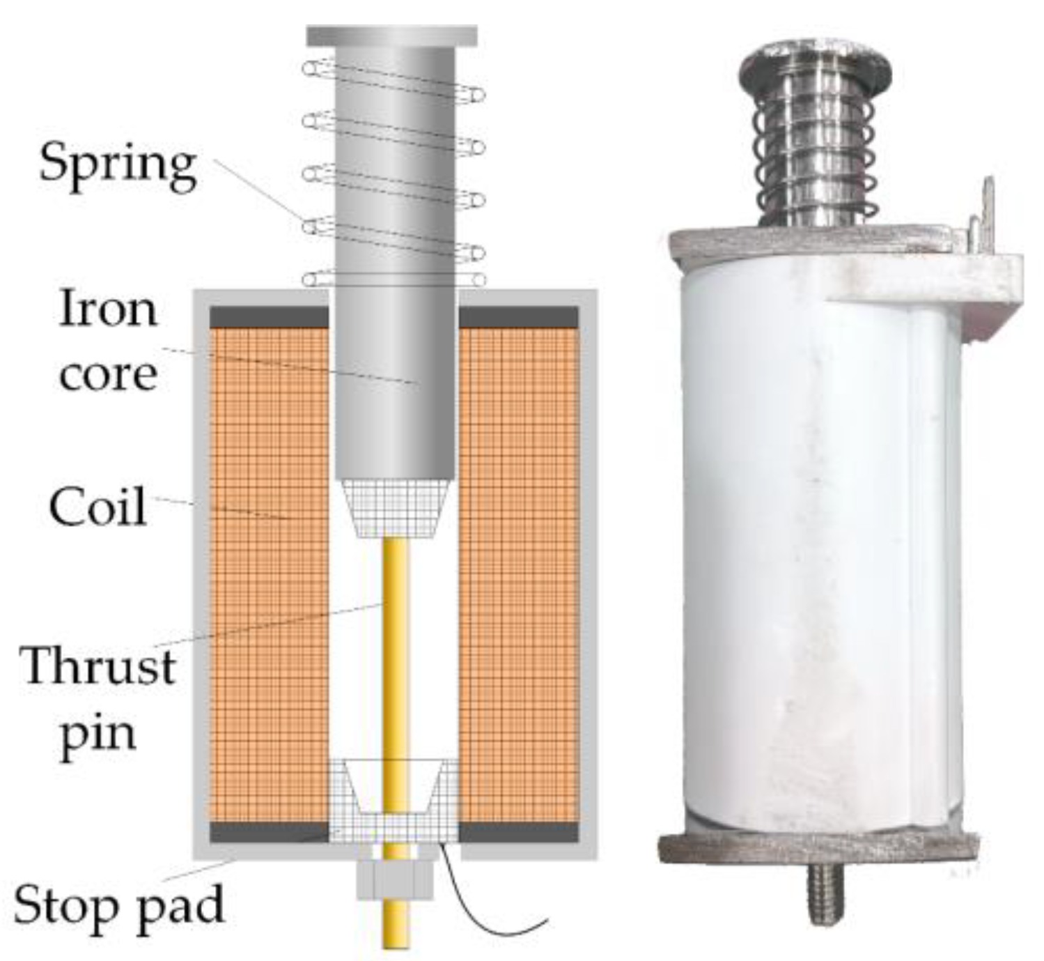
The push–pull electromagnet is a common solenoid actuator, and its mechanical structure is mainly composed of an excitation coil, a movable iron core and a spring. When there is no current in the coil, the iron core will form an extended state under the action of the spring. When a current is applied to the coil in any direction, the iron core will move to the center of the coil, thereby forming a retracted state of the electromagnet. Figure 1 shows the structure diagram of the push–pull electromagnet without the ferromagnetic shell.

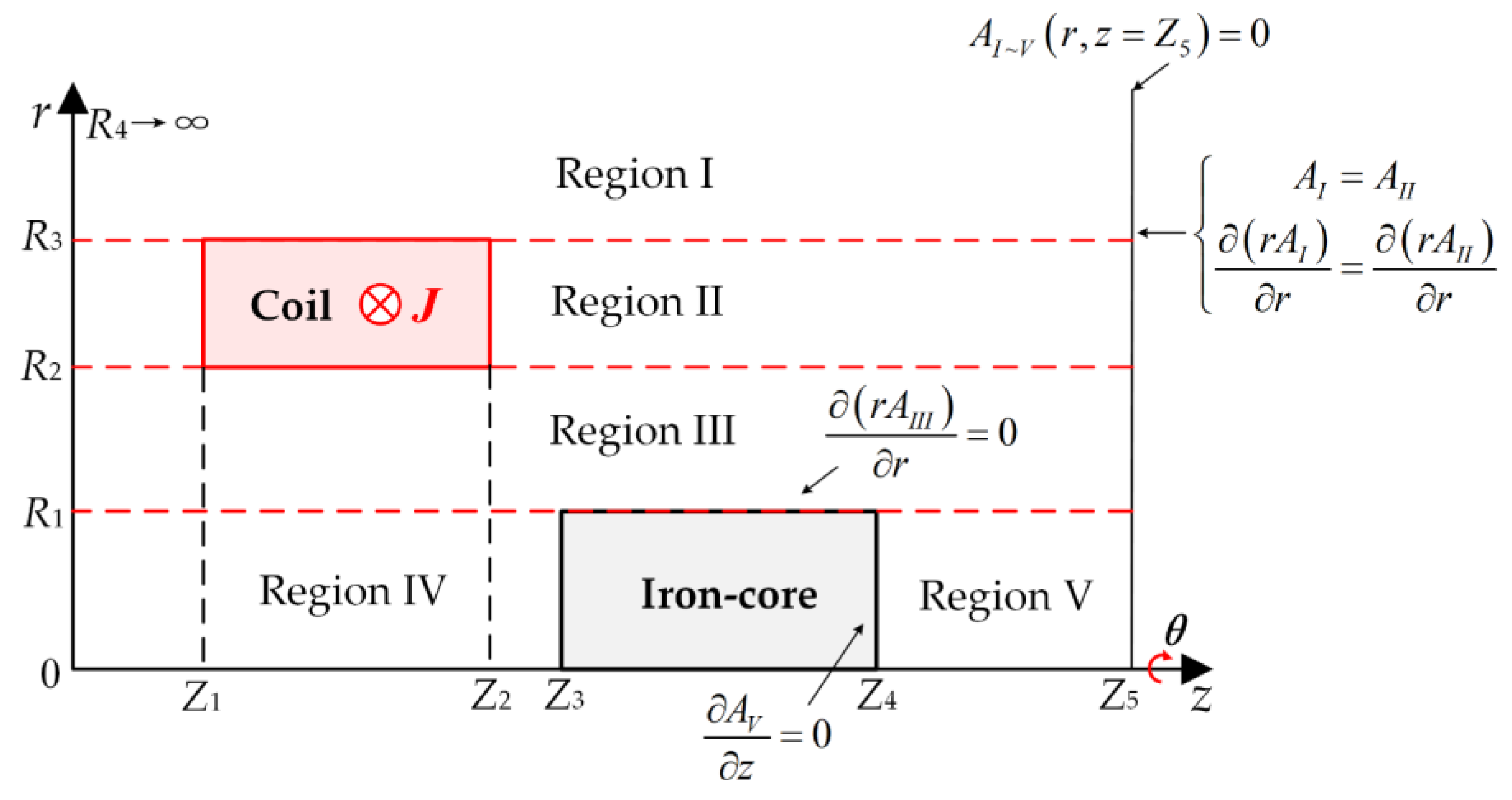
As shown in Figure 1, the ring at the top of the iron core is used to assemble the spring, the ring is always away from the center of the coil during the operation of the solenoid, and the thrust pin is made of carburized weakly magnetic stainless steel, which is assumed to have a negligible impact on the magnetic field, and therefore the iron core can be analyzed as a standard ferromagnetic cylinder. The modeling of the solenoid actuator magnetic field subdomain method assumes that the magnetic permeability of the iron core is infinite, that is, that the magnetic field lines on the iron core are all perpendicular to the surface of the iron core. In the calculation, the tangential component of the magnetic field is set at its boundary as zero. The magnetic field subdomain method modeling of the solenoid actuator and the setting of boundary conditions are shown in Figure 2.

Since the solenoid actuator is cylindrical and the magnetic field has axial symmetry characteristics, it is suitable to use the magnetic vector potential equation in cylindrical coordinates to solve. Take the central axis of the iron core as the Z-axis and the radial direction as the R-axis. The entire solution domain is limited to three outer boundaries $\left(r,z=0\right)$, $\left(r\to \infty ,z\right)$ and $\left(r,z=Z_5\right)$, assuming that the magnetic vector potential on the boundaries is equal to zero. For more accurate solution results, each outer boundary should be kept away from the coil and the movement area of the iron core. The five sub-domains into which the magnetic field is divided are the air region above the coil (Region I), the air region to the left and right of the coil (Region II), the air gap region between the coil and the iron core (Region III), the air region to the left of the iron core (Region IV) and the air region to the right of the iron core (Region V).

Compared to solving for a three-dimensional magnetic field using Maxwell’s equations, the magnetic field of the solenoid has rotational symmetry, and the rotation of the magnetic induction intensity only has the $\theta$ component, the magnetic vector $\mathit{A}$ has only the $\theta$ component and its magnitude is related to the coordinates of $r$ and $\mathit{z}$, as shown in (2). Then, the magnetic vector can be expressed as $A_{\theta }$ or $A\left(r,z\right)$.

$${\nabla }^2\mathit{A}=-{\left(\nabla \times \mathit{B}\right)}_{\theta }=-\frac{\partial B_r}{\partial z}+\frac{\partial B_z}{\partial r}=-{\mu }_0\mathit{J}$$

(1)

The three components of solenoid magnetic induction intensity in the cylindrical coordinate system are [18]

$$B_r\left(r,\mathrm{z}\right)=-\frac{\partial A_{\theta }}{\partial z},B_{\theta }=0,B_z\left(r,\mathrm{z}\right)=\frac{1}{r}\frac{\partial \left(r{A}_{\theta }\right)}{\partial r}$$

(2)

Substituting (3) into (2), it is obtained that the magnitude and potential $\mathit{A}$ of the solenoid actuator satisfy

$${\nabla }^2\mathit{A}=\frac{{\partial }^2{A}_{\theta }}{\partial r^2}+\frac{1}{r}\frac{\partial A_{\theta }}{\partial r}-\frac{A_{\theta }}{r^2}+\frac{{\partial }^2{A}_{\theta }}{\partial z^2}=-{\mu }_{0}J\left(r,z\right)$$

(3)

where ${\mu }_0$ is the permeability in air and $J$ is the current density in the coil. Express the current density as a function $J\left(r,z\right)$ related to $r$, $z$ in order to distinguish the air regions where the current density is zero, and then distinguish the application area of Poisson equation and Laplace equation.

Solve the homogeneous differential equation using the separation of variables method. Let $A_{\theta }\left(r,z\right)=R\left(r\right)Z\left(z\right)$ and substitute it into (4) and multiply both sides by $1/RZ$ to obtain

$$\frac{1}{Z}\frac{{\partial }^{2}Z}{\partial z}-\frac{1}{r^2}+\frac{1}{r}\cdot \frac{1}{R}\frac{\partial R}{\partial r}+\frac{1}{R}\frac{{\partial }^{2}R}{\partial r^2}=0$$

(4)

Assuming that $\frac{1}{Z}\frac{{\partial }^{2}Z}{\partial z}=-{\alpha }^2$, its particular solution is $x=\alpha r$, substituting into (5) to obtain

$$\left\{\begin{array}{c}\frac{{\partial }^{2}Z}{\partial z}+{\alpha }^{2}Z=0\\ \frac{{\partial }^{2}R}{\partial x^2}+\frac{1}{x}\frac{\partial R}{\partial x}-\left(1+\frac{1}{x^2}\right)R=0\end{array}\right.$$

(5)

From $Z\left(0\right)=0$ and $Z\left(\infty \right)=0$, can know that $Z$ is not a mediocre solution and ${\alpha }^2>0$, the above formula of (6) is a second-order constant coefficient homogeneous differential equation and the general solution satisfies

$$Z\left(z\right)=c_1\cos \left(\alpha z\right)+c_2\sin \left(\alpha z\right)$$

(6)

The following formula of (6) conforms to the form of a first-order imaginary Bessel function (also known as modified Bessel function), and its general solution is

$$R\left(x\right)=c_3{I}_1\left(x\right)+c_4{K}_1\left(x\right)$$

(7)

where $c_1~c_4$ are constants, $I_1$ represents the first-order modified Bessel function and $K_1$ represents the first-order modified Bessel function of the second kind.

Substitute $x=\alpha r$ into (8) and $A_{\theta }\left(r,z\right)=R\left(r\right)Z\left(z\right)$ to obtain the general solution equation of the magnetic vector potential in the region I~V and then

$$A_{\theta }\left(r,z\right)={\displaystyle \sum _{n=1}^{\infty }\left[c_1\cos \left({\alpha }_{n}z\right)+c_2\sin \left({\alpha }_{n}z\right)\right]}\left[c_3{I}_1\left({\alpha }_{n}r\right)+c_4{K}_1\left({\alpha }_{n}r\right)\right]$$

(8)

According to the convergence and divergence of the modified Bessel function of the magnetic vector potential of the cylindrical coordinate system at the outer boundary of the magnetic field, the general solution form of the simplified magnetic vector potential of each subdomain can be obtained, respectively.

$$\left\{\begin{array}{l}{A}_I\left(r,z\right)={\displaystyle \sum _{n=1}^{\infty }{b}_n^I{K}_1\left(a_{n}r\right)}\sin \left(a_{n}z\right)\hfill \\ A_{II}\left(r,z\right)={\displaystyle \sum _{n=1}^{\infty }\left\{a_n^{II}{I}_1\left(a_{n}r\right)+b_n^{II}{K}_1\left(a_{n}r\right)-C_n{L}_1\left(a_{n}r\right)\right\}}\sin \left(a_{n}z\right)\hfill \\ A_{III}\left(r,z\right)={\displaystyle \sum _{n=1}^{\infty }\left\{a_n^{III}{I}_1\left(a_{n}r\right)+b_n^{III}{K}_1\left(a_{n}r\right)\right\}}\sin \left(a_{n}z\right)\hfill \\ A_{IV}\left(r,z\right)={\displaystyle \sum _{k=1}^{\infty }{a}_k^{IV}{I}_1\left({\beta }_{k}r\right)}\sin \left({\beta }_{k}z\right)\hfill \\ A_V\left(r,z\right)={\displaystyle \sum _{k=1}^{\infty }{a}_k^V{I}_1\left({\lambda }_{k}r\right)}\cos \left({\lambda }_k\left(z-Z_4\right)\right)\hfill \end{array}\right.$$

(9)

where

$$C_n={\mu }_0\left(\pi /2\right)J_n{\alpha }_n^{-2},J_n=\frac{2J}{n\pi }\left(\cos \left({\alpha }_n{Z}_1\right)-\cos \left({\alpha }_n{Z}_1\right)\right)$$

(10)

and $n$ is a positive integer, $k$ is a positive odd number and ${\mu }_0$ is the magnetic permeability of air, taking $4\pi \times {10}^{-7}$ H/m. Substitute the external boundary conditions into (10) to obtain ${\alpha }_n=n\pi /Z_5$, ${\lambda }_k=k\pi /\left(2\left(Z_5-Z_4\right)\right)$. $I_0$ is the zero order modified Bessel functions, $K_0$ is the zero-order modified Bessel function of the second kind and $L_0$, $L_1$ are the zero and first-order modified Struve functions. $b_n^I$, $a_n^{II}$, $b_n^{II}$, $a_n^{III}$, $b_n^{III}$, $a_k^{IV}$ and $a_k^V$ are the integral coefficients of each region, determined by the interface conditions.

By further substituting the inter-domain boundary conditions into (10) to obtain

$$a_n^{II}={\alpha }_n{R}_3{C}_n\left(L_0\left({\alpha }_n{R}_3\right)K_1\left({\alpha }_n{R}_3\right)+L_1\left({\alpha }_n{R}_3\right)K_0\left({\alpha }_n{R}_3\right)\right)$$

(11)

$$b_n^{II}=b_n^I+{\alpha }_n{R}_3{C}_n\left(L_1\left({\alpha }_n{R}_3\right)I_0\left({\alpha }_n{R}_3\right)-L_0\left({\alpha }_n{R}_3\right)I_1\left({\alpha }_n{R}_3\right)\right)$$

(12)

$$a_n^{III}=a_n^{II}-{\alpha }_n{R}_2{C}_n\left(L_1\left({\alpha }_n{R}_2\right)K_0\left({\alpha }_n{R}_2\right)+L_0\left({\alpha }_n{R}_2\right)K_1\left({\alpha }_n{R}_2\right)\right)$$

(13)

$$b_n^{III}=b_n^{II}+{\alpha }_n{R}_2{C}_n\left(L_0\left({\alpha }_n{R}_2\right)I_0\left({\alpha }_n{R}_2\right)-L_1\left({\alpha }_n{R}_2\right)I_0\left({\alpha }_n{R}_2\right)\right)$$

(14)

$$a_n^{III}-b_n^{III}\frac{K_0\left({\alpha }_n{R}_1\right)}{I_0\left({\alpha }_n{R}_1\right)}={\displaystyle \sum _{k=1}^{\infty }\left(a_k^{IV}\frac{k}{n{Z}_3}\frac{I_0\left({\beta }_k{R}_1\right)}{I_0\left({\alpha }_n{R}_1\right)}f\left(n,k\right)+a_k^V\frac{k}{n\left(Z_5-Z_4\right)}\frac{I_0\left({\lambda }_k{R}_1\right)}{I_0\left({\alpha }_n{R}_1\right)}g\left(n,k\right)\right)}$$

(15)

$$a_k^{IV}=\frac{2}{Z_3}{\displaystyle \sum _{n=1}^{\infty }\left(a_n^{III}\frac{I_1\left({\alpha }_n{R}_1\right)}{I_1\left({\beta }_k{R}_1\right)}+b_n^{III}\frac{K_1\left({\alpha }_n{R}_1\right)}{I_1\left({\beta }_k{R}_1\right)}\right)}\times f\left(n,k\right)$$

(16)

$$a_k^V=\frac{2}{Z_5-Z_4}{\displaystyle \sum _{n=1}^{\infty }\left(a_n^{III}\frac{I_1\left({\alpha }_n{R}_1\right)}{I_1\left({\lambda }_k{R}_1\right)}+b_n^{III}\frac{K_1\left({\alpha }_n{R}_1\right)}{I_1\left({\lambda }_k{R}_1\right)}\right)}\times g\left(n,k\right)$$

(17)

where

$$f\left(n,k\right)=\left\{\begin{array}{cc}-\frac{{\alpha }_n\sin \left(k\pi /2\right)\cos \left({\alpha }_n{Z}_3\right)}{\left({\alpha }_n^2-{\beta }_k^2\right)}\hfill & \hfill for\hspace{0.33em}{\alpha }_n\ne {\beta }_k\\ 0.5\times Z_3\hfill & \hfill \hspace{0.33em}for\hspace{0.33em}{\alpha }_n={\beta }_k\end{array}\right.$$

(18)

$$g\left(n,k\right)=\left\{\begin{array}{cc}-\frac{{\alpha }_n\cos \left({\alpha }_n{Z}_4\right)}{\left({\alpha }_n^2-{\lambda }_k^2\right)}& \hfill \hspace{0.33em}for\hspace{0.33em}{\alpha }_n\ne {\lambda }_k\\ 0.5\times \left(Z_5-Z_4\right)\sin \left({\alpha }_n{Z}_4\right)\hfill & \hfill \hspace{0.33em}for\hspace{0.33em}{\alpha }_n={\lambda }_k\end{array}\right.$$

(19)

Note that the computation of the magnetic vector potential in each subdomain contains an infinite number of series, and in order to truncate the number of series, it is necessary to define the maximum number of harmonic terms N_max and K_max, whose values are larger the longer the computation will take. With the gradual convergence of the calculation results, the effect of increasing N_max and K_max on the calculation results will become smaller and smaller. Therefore, when setting the specific values of N_max and K_max, the time-consuming and calculation accuracy requirements are taken into account.

When solving, first calculate $a_n^{II}$ and $a_n^{III}$ directly by (12) and (14), and then substitute $a_n^{III}$ into (16)–(18) and expand the sum series into matrix form to solve $b_n^{III}$, $a_k^{IV}$ and $a_k^V$, and finally substituting $b_n^{III}$ into (13) and (15) to obtain $b_n^I$ and $b_n^{II}$. When all the coefficients are known, the magnetic vector potential in the whole solution domain can be obtained by substituting into (10).

2.2. Inductance Equation Based on Subdomain Method

The inductive energy storage of the solenoid actuator is distributed in the conductive medium, and its total magnetic energy formula is

$$\frac{1}{2}{L}_m{I}^2=\frac{1}{2}{\displaystyle \underset{V}{\int }A\cdot Jdv}$$

(20)

where $L_m$ is the inductance value with iron core, $I$ is the current in the coil and $V$ is the volume of the conductor.

Assuming that the current in the coil is evenly distributed on the rectangular section of the coil, the current density value is equal to the current value divided by the area of the rectangular section and the inductance value of the iron core is

$$L_m=\frac{2\pi N^2}{{\left(R_3-R_2\right)}^2{L}^{2}J}{\displaystyle \sum _{n=1}^{\infty }\left\{\begin{array}{l}\frac{\pi }{2{\alpha }_n^2}\left(\begin{array}{c}{a}_n^{II}\left(R_3{U}_n\left(R_3\right)-R_2{U}_n\left(R_2\right)\right)\\ +b_n^{II}\left(R_3{V}_n\left(R_3\right)-R_2{V}_n\left(R_2\right)\right)\\ -C_n\frac{{\alpha }_n^3}{3{\pi }^2}\left(R_3^4{W}_n\left(R_3\right)-R_2^4{W}_n\left(R_2\right)\right)\end{array}\right)\\ \cdot \left(\cos \left({\alpha }_n{Z}_1\right)-\cos \left({\alpha }_n{Z}_2\right)\right)\end{array}\right\}}$$

(21)

where

$$\left\{\begin{array}{c}{U}_n\left(r\right)=I_1\left({\alpha }_{n}r\right)L_0\left({\alpha }_{n}r\right)-I_0\left({\alpha }_{n}r\right)L_1\left({\alpha }_{n}r\right)\\ V_n\left(r\right)=K_1\left({\alpha }_{n}r\right)L_0\left({\alpha }_{n}r\right)-K_0\left({\alpha }_{n}r\right)L_1\left({\alpha }_{n}r\right)\\ W_n\left(r\right)=F\left(1,2;3/2,5/2,3;{\alpha }_n^2{r}^2/4\right)\end{array}\right.$$

(22)

and $L$ is coil length, $N$ is coil turns and $F$ represents hypergeometric function.

From (22), it can be seen that, when the structural dimensions of the coil and the iron core are known, as long as the instantaneous position of the movable iron core and the current in the coil are known, the inductance value of the corresponding position can be obtained by the magnetic field subdomain method. In fact, when the B-H curve is not considered, the inductance value has nothing to do with the current, and the calculated inductance of the subdomain method also does not change with the current.

2.3. Electromagnetic Characteristics Analysis of the Push–Pull Electromagnet

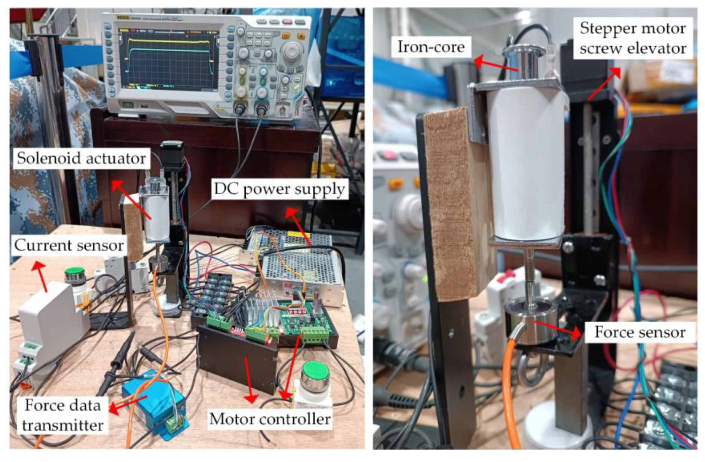
In order to verify the accuracy of the inductance calculation, an ANSYS EM 19.1 simulation model was built according to the structural parameters of the push–pull electromagnet in Figure 1, and wrote a MATLAB numerical calculation program. The parameters are shown in

Table 1. Analysis parameters of an electromagnetic actuator.

Symbol	Quantity	Value
R1	Radius of the iron	5.9 mm
R2	Inner radius of the coil	7.4 mm
R3	Outer radius of the coil	12.0 mm
R4	Radial boundary of the solution domain	50.0 mm
L	Axial length of the coil	52 mm
l	Axial length of the iron core	58 mm
h	Relative displacement of coil and armature center	variable
Z1	Axial position of the coil (left side)	74 mm
Z3	Axial position of the iron-core (left side)	53.7 mm
Z5	Outer boundary of the coil	200 mm
N	Number of turns of the coil	720
Nmax	Number of harmonic terms in region I, II and III	40
Kmax	Number of harmonic terms in region IV and V	40

.

The dimensional parameters in Table 1 were measured by vernier calipers after disassembling the electromagnetic actuator shown in Figure 1. The number of turns of the coil N is provided by the manufacturer, and the excitation current I is the maximum allowable current calculated from the rated operating conditions of the electromagnetic actuator. The boundary condition Z₅ and the number of harmonic terms N_max and K_max were defined to obtain the results, and these values have been obtained to be large enough, as further increasing these values will have little effect on the simulation results of the subdomain method and FEM.

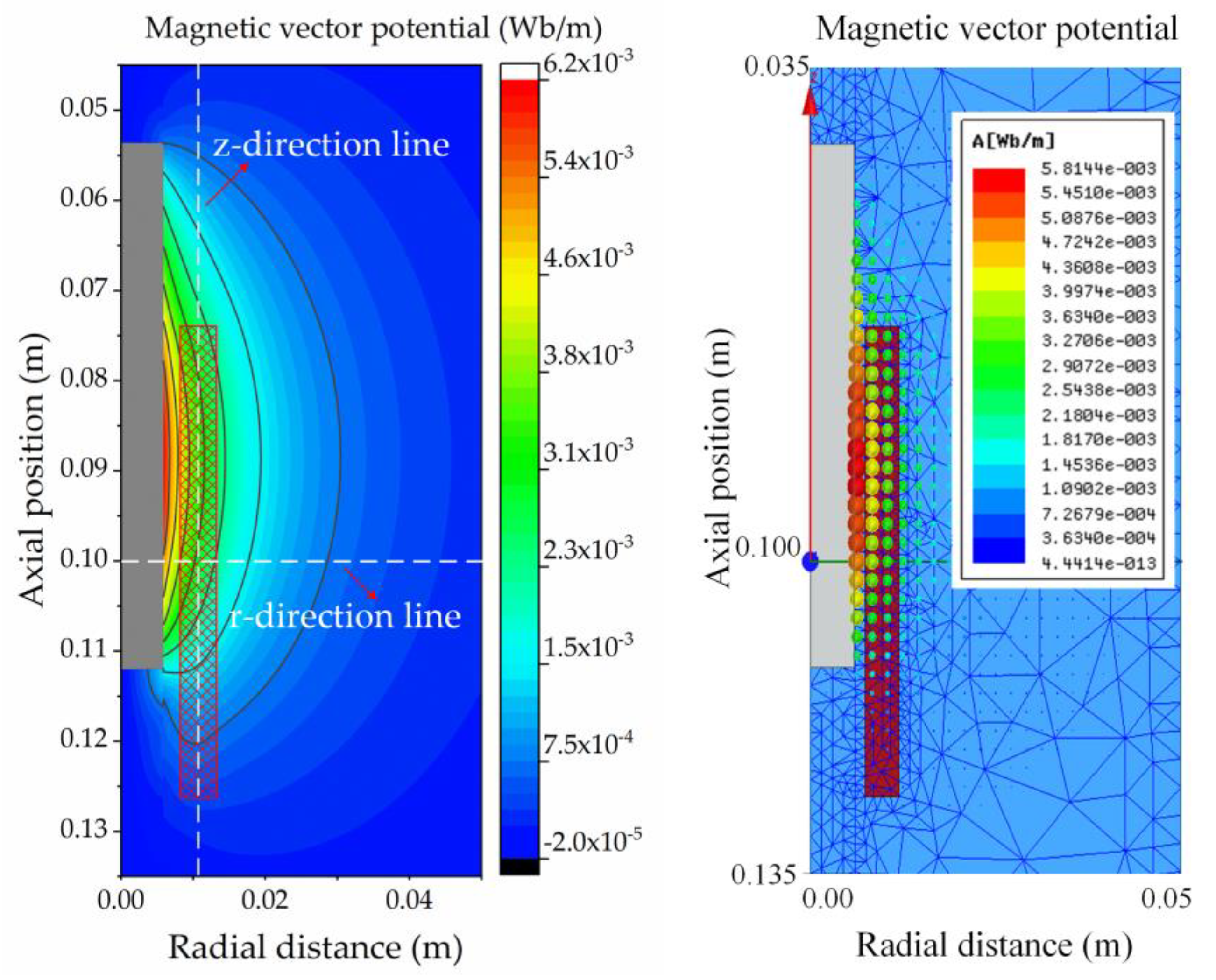
When the excitation current in the coil is given to be 7.24 A, the magnetic vector potential distribution plot calculated by the subdomain method is compared with the FEM results, as shown in Figure 3, where only the data of 0.035 m to 0.135 m in the 0.2 m axial computational domain are shown for easy observation, where the permeability of the iron core material in the FEM is set to electrical iron (DT4, a standard steel in China).

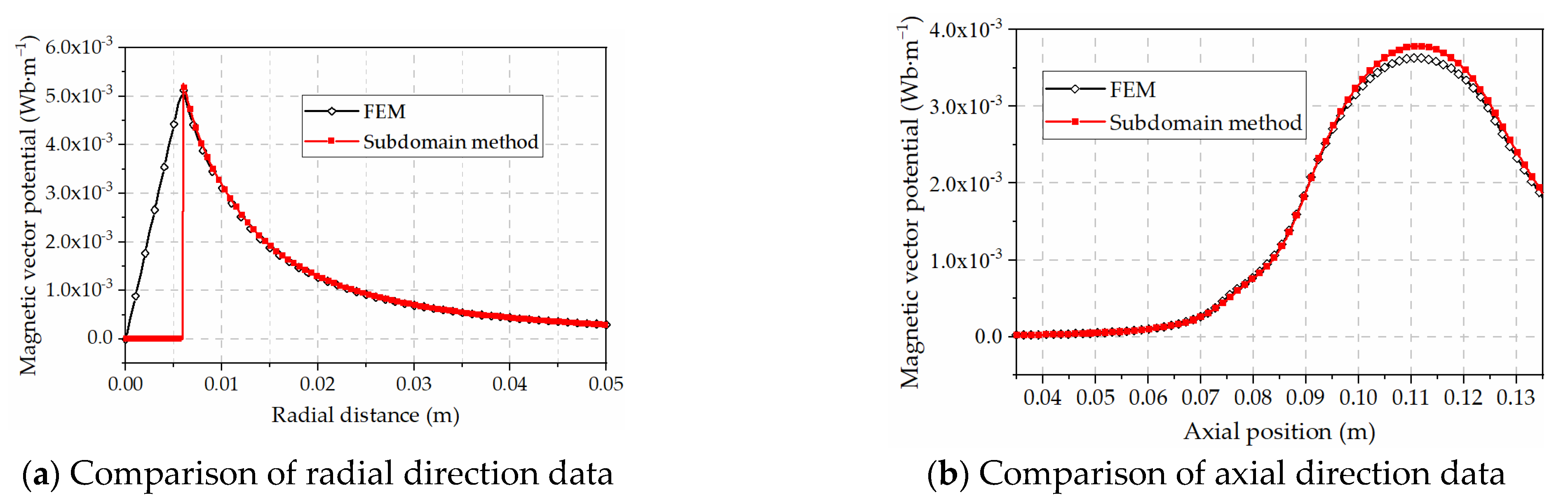
The peak magnetic vector potential data in Figure 3 are 6.16 × 10⁻³ Wb/m and 5.81 × 10⁻³ Wb/m, respectively, with a difference of about 5.9%. However, it is difficult to obtain a valid global data comparison by the naked eye with this color representation. Therefore, we take the data comparison on the picture on two lines; one is in the r-direction pointing from the center of the coil to the radial boundary as shown in Figure 4a, and the other is in the z-direction in the middle of the inner and outer diameters of the coil, as shown in Figure 4b.

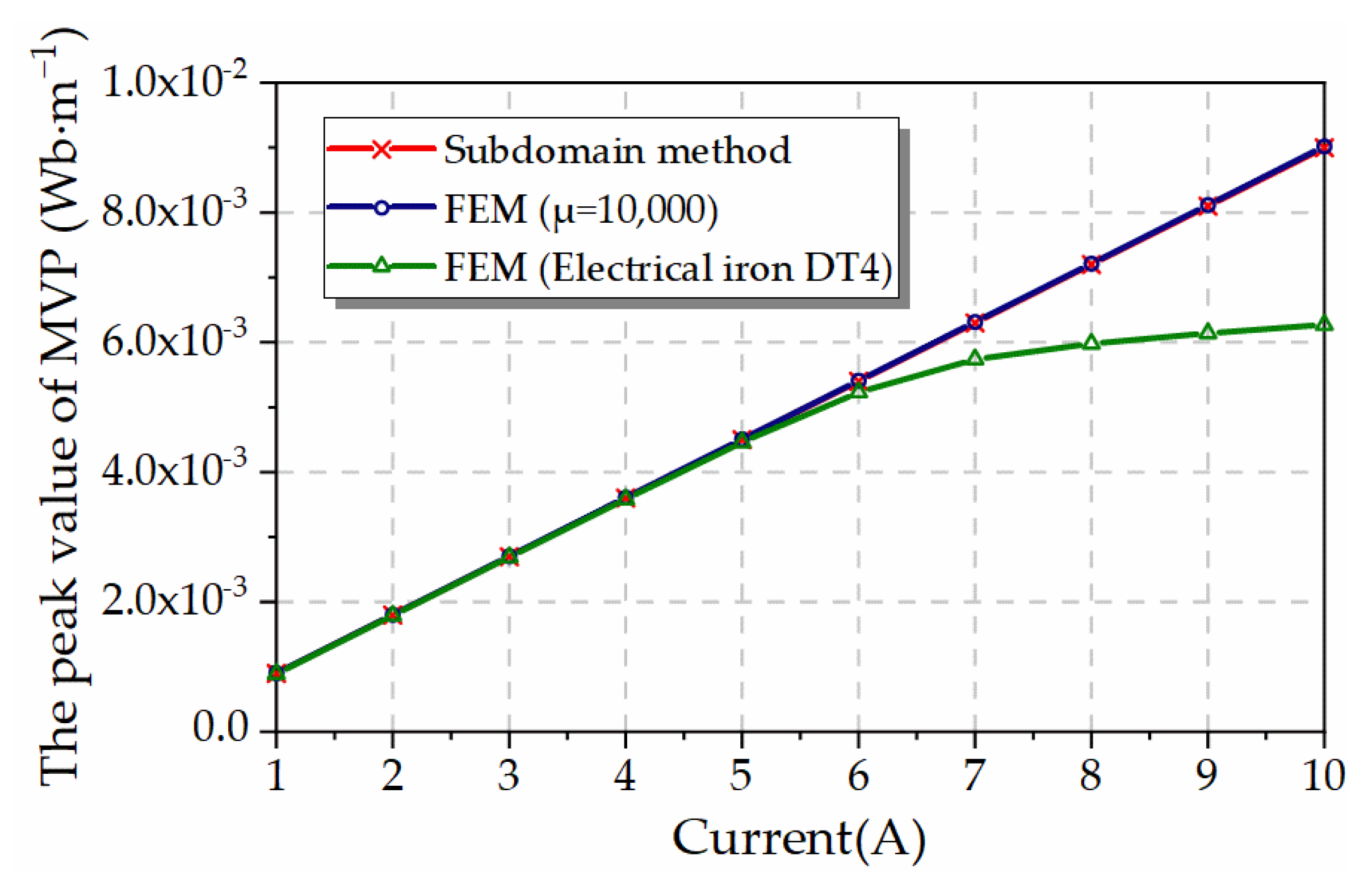
In fact, the size of the excitation current is necessarily related to the degree of magnetic saturation. In order to specifically analyze the accuracy of the calculation of the magnetic vector potential, different sizes of the excitation current are applied to the coil, while a set of magnetic permeability of a constant value of 10,000 is added to the FEM, and the results of the comparison of the peak vector potential are shown in Figure 5.

As can be seen in Figure 5, with the increase in current, the peak magnetic vector potentials calculated by the subdomain method and the magnetic permeability set to 10,000 in the FEM are basically equal, which indicates that the calculation results of the subdomain method are very approximately equal to the case of the magnetic core permeability set to a large amount in the FEM. When the core material in the FEM is electrician’s soft iron (DT4), the calculation result is not increased linearly, but increased according to the trend of the B-H curve, which indicates that, with the gradual magnetic saturation of the iron core, the error of the calculation result of the sub-domain method is increased. In order to avoid overheating damage, the solenoid actuator usually does not pass a large current, so in general the results of the subdomain method can be adopted.

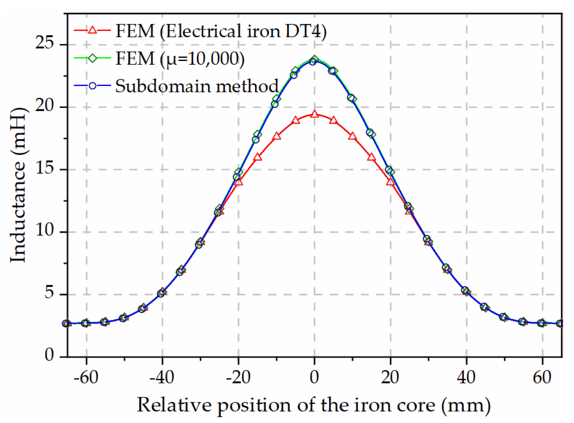
The comparison of the inductance curves of the movable iron core at different axial positions relative to the center of the coil is shown in Figure 6, and a data point is taken every 0.5 mm. Among them, the magnetic permeability of the iron core in the finite element is calculated according to the constant value of 10,000 and the B-H curve of electrical iron (DT4) [5].

It can be seen from Figure 6 that the inductance calculated by the subdomain method is basically the same as the result when the relative magnetic permeability in the FEM is 10,000, which shows that the calculation of subdomain method is accurate when the iron core has high magnetic permeability and does not consider magnetic saturation. When the core is calculated according to the B-H curve of the electrical iron (DT4), the closer the relative position of the iron core and the coil is, the greater the difference in the calculated inductance, which means that, when the iron core and the coil are in these relative positions, the 7.24 A current excitation has caused the magnetic core to create a slight magnetic saturation.

After the inductance curve is obtained, the EMF on the iron core can be calculated through the change in the inductance gradient. Use the virtual displacement method to solve the kinematic process. The EM energy of the system is [14]

$$W=\frac{1}{2}L(x)·i^2(t)$$

(23)

where $W$ is the magnetic induction energy, $L\left(x\right)$ is the inductance value related to the position of the movable iron core, $i\left(t\right)$ is the excitation current of the coil and the EMF that the iron core receives in the axial direction of the coil is [15]

$$F_{mag}=\frac{\mathrm{d}W}{\mathrm{d}x}=\frac{1}{2}{i}^2(t)·\frac{\partial L(x)}{\partial x}$$

(24)

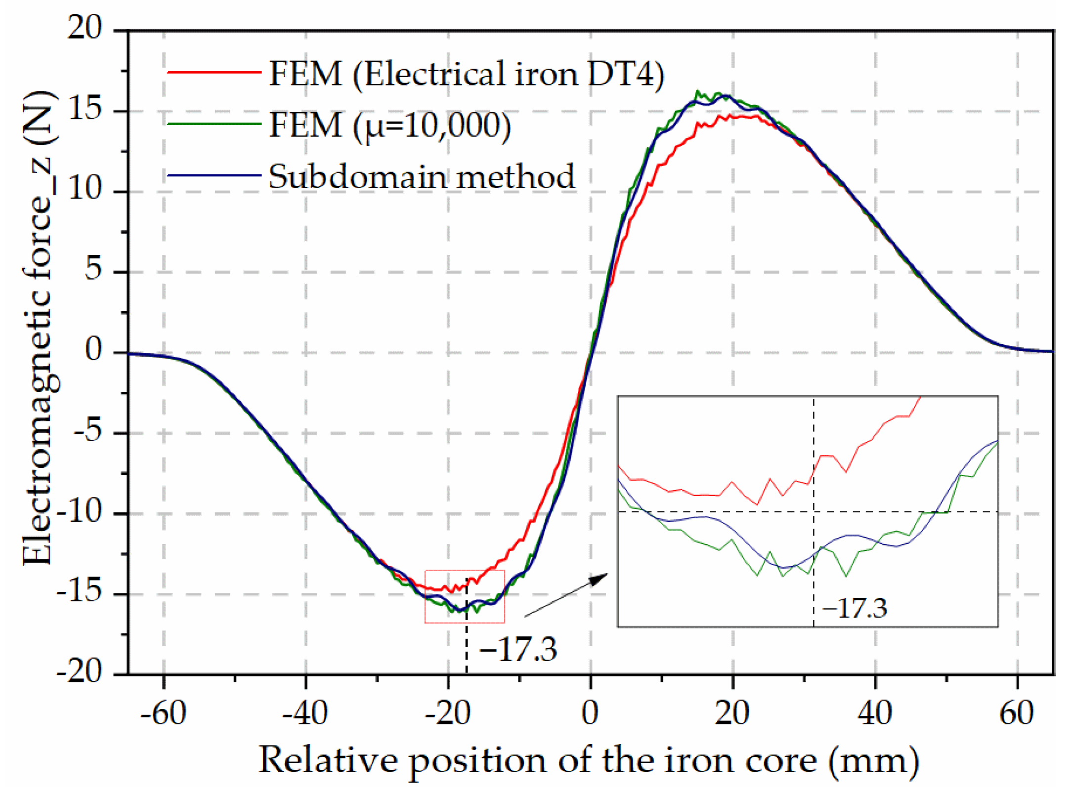
The EMF comparison of the movable iron core at different axial positions relative to the coil is shown in Figure 7.

When the coil is energized, the direction of EMF on the iron core always points to the center of the coil. As the electromagnet shown in Figure 1, take the point where the center of the coil and the iron core coincide as the coordinate origin. Defining the EMF in the upward direction as positive, the iron core is subjected to a downward negative force when it is located above the coil, and a positive force if the iron core is located below the coil. As can be seen from the enlarged diagram in Figure 7, the EMF obtained by the FEM is irregularly jagged, which is due to the finite difference calculation, while the EMF calculated by the subdomain method is wavy, which is due to the limitation of the number of harmonic terms.

3. Experimental Platform Construction and Algorithm Verification

3.1. Verification of the Calculated Electromagnetic Force

In order to verify the accuracy of the magnetic field subdomain method to calculate the EMF of the solenoid actuator, an EMF test experimental platform was built. In this stage of the experiment, the spring was disassembled and the influence of the spring force was eliminated.

For accurate analysis, the experimental platform in this study is arranged longitudinally, which can reduce the errors caused by the friction force and the eccentricity of the magnetic core. Use the stepper motor lifting platform to adjust the iron core to move down to the specified position in Table 1. In order to avoid errors caused by the force sensor’s own gravity and installation preload on the test results, the transmitter should be zeroed before the test. This operation also eliminates the gravity of the iron core.

The experimental platform for testing the EMF is shown in Figure 8. Apply 12 VDC to the coil, and the current data detected by the current sensor and the EMF data detected by the force sensor are shown in Figure 9.

The reason that the current gradually reaches the preset value in Figure 9 without overshooting is that the inductance of the coil acts as a suppressor of the sudden change in current. On the other hand, the EMF overshoots at start and stop, which is due to the fact that the system in the experimental setup does not have the desired rigidity. Under the action of the impact EMF, the cantilever on which the force sensor is mounted elastically deforms and begins to vibrate, and as it stabilizes the deformation recovers, which leads to an overshoot of the EMF test value.

In the experiment, the average current after stabilization is 7.24 A, the average EMF after stabilization is 14.7 N, the EMF calculated by the subdomain method is 15.8 N and the FEM result using electrical iron (DT4) is 14.3 N. If the EMF measured in the experiment is used as the benchmark, the calculation accuracy of the FEM and the subdomain method are 97% and 93%, respectively.

The semi-analytical method has the advantage of flexible calculation. It can calculate the dynamic EMF according to the changing current, which is helpful to study the EMF dynamic response characteristics of the solenoid actuator. The varying current can be measured by a sensor or calculated by a circuit with a resistive inductive load. The comparison between the EMF calculated according to the tested current and the EMF directly tested by the force sensor in the experiment is shown in Figure 10.

Since the test values of both EMF and current are not constants, they usually have different amplitudes of noise. Since the subdomain method does not directly substitute the constant excitation 7.24 A when calculating, but substitutes the current waveform tested in the experiment, the results obtained also have noise. As can be seen from Figure 10, the results calculated by the subdomain method are closer to the experimental results.

3.2. Verification of the Calculated Output Thrust

The above analysis shows the accuracy of the subdomain method for calculating the EMF, but in practical applications, the output thrust of the push–pull electromagnet is the most concerned by the users, so the force of the spring and the gravity of the iron core must be considered. Compared with the FEM, the semi-analytical method can better deal with these factors that affect the output thrust and realize the calculation.

To verify the accuracy of the output thrust calculations, we performed a spring force test, as shown in Figure 11, and an output thrust test, as shown in Figure 12.

The force sensor transmitter is zeroed and then connected with the iron core using a connecting nut. At this time, if the solenoid is energized, the force measured by the force sensor is a resultant of the spring force, the core gravity and the EMF, which is also the output thrust when the push–pull electromagnet is arranged longitudinally. Taking the downward direction as the positive direction, the output thrust is expressed as

$$F_t=F_{mag}+M+F_s$$

(25)

where $M$ is the gravity of the iron core, $F_s=-kx$ is the spring force, $x$ is the compression of the spring and $k$ is the force coefficient of the spring.

Since the force coefficient $k$ of the tested spring is unknown, it is necessary to obtain the force of the spring at different degrees of compression throughout the experiment. The spring force test experimental platform is shown in Figure 11. During the test, the coil is not energized. The stepper motor lifting platform is moved down at a constant speed and the pressure sensor compresses the spring at a constant speed. During this test process, the force detected by the sensor is $\left(M-kx\right)$, which is already considered the gravity of the iron core. The force sensor detects the spring force waveform corresponding to different compression amounts (the data are Savitzky–Golay-smoothed [19]), as shown in Figure 13.

The working stroke of the push–pull electromagnet used in the experiment is 12.7 mm, and the relative position of the movable iron core and coil is −25.5 mm~−12.8 mm, and the EMF obtained by the subdomain method in the corresponding interval in Figure 7 is taken to be subtracted from the spring force to obtain the actual output thrust of the iron core. The calculation results are shown in Figure 14.

It can be seen from Figure 14 that, when the push rod is lowered to the specified position, the calculated theoretical output thrust of the push–pull electromagnet should be 12.6 N. The current and thrust waveform displayed by the oscilloscope in the experiment are shown in Figure 15.

Due to the spring force, the force sensor detects the upward pulling force before the solenoid is energized, and when we set the sensor to output positive data when under pressure, the pulling force is correctly displayed as a negative value. Since the subdomain method does not consider the magnetic saturation, the calculated value of the EMF will be larger than the actual value when the excitation current of the electromagnet is larger, which is 12.6 N, while the total output EMF of the experimental test is 11.2 N. Taking the latter as the benchmark, the accuracy of the subdomain method results is 87%.

4. Conclusions

A solenoid actuator is a typical EM energy and mechanical energy conversion device. Although it has been widely used in many industrial applications, the magnetic field calculation of solenoids with movable iron cores has always been a difficult research point. The calculation at this stage is basically handled by finite element analysis, and there are many drawbacks to this. In this study, the EM characteristic data of the solenoid actuator are calculated by the magnetic field subdomain method. When the excitation current applied to the coil is 7.24 A, the accuracy of calculating the EMF is 93%.

Compared with the FEM, the magnetic field subdomain method has the advantages of programmable and flexible calculation. Using these advantages, many calculations that cannot be processed by the FEM can be realized, such as the construction of intelligent algorithms such as genetic algorithms to optimize the design parameters of EM actuators. In this study, the calculation of the iron core output thrust of a push–pull EM actuator without a ferromagnetic shell is realized by MATLAB programming, and the calculation accuracy is 87%. The disadvantage is that the magnetic permeability of the iron core is regarded as infinite in the calculation process, the influence of the eddy current on the surface of the iron core is ignored and the calculation accuracy will be reduced in the case of a high-current strong magnetic field or low-magnetic-permeability iron core.

References

1. Afshar, S.; Khamesee, M.B.; Khajepour, A. Optimal configuration for electromagnets and coils in magnetic actuators. IEEE Trans. Magn. 2012, 49, 1372–1381. [Google Scholar] [CrossRef]
2. Hassannia, A.; Abedi, K. Optimal switching scheme for multistage reluctance coilgun. IEEE Trans. Plasma Sci. 2021, 49, 1241–1246. [Google Scholar] [CrossRef]
3. Lu, M.; Zhang, J.; Yi, X.; Zhuang, Z. Advanced mathematical calculation model of single-stage RCG. IEEE Trans. Plasma Sci. 2022, 50, 1026–1031. [Google Scholar] [CrossRef]
4. Lequesne, B. Automotive electrification: The nonhybrid story. IEEE Trans. Transp. Electr. 2015, 1, 40–53. [Google Scholar] [CrossRef]
5. Wu, S.; Zhao, X.; Li, C.; Jiao, Z.; Qu, F. Multiobjective optimization of a hollow plunger type solenoid for high speed on/off valve. IEEE Trans. Ind. Electron. 2017, 65, 3115–3124. [Google Scholar] [CrossRef]
6. Li, K.; Luo, C.; Niu, F.; Li, C.; Tong, M.; Wu, Y. A new magnetic release design with high anti-interference capability. IEEE Trans. Magn. 2021, 57, 4001009. [Google Scholar] [CrossRef]
7. Cao, Z.; Zuo, Y. Electromagnetic riveting technique and its applications. Chin. J. Aeronaut. 2020, 33, 5–15. [Google Scholar] [CrossRef]
8. Hogan, P.H.; Van de Ven, J.D. Dynamic modeling of a linear electromagnetic piston pump. In Fluid Power Systems Technology; American Society of Mechanical Engineers: New York, NY, USA, 2017; p. V001T01A062. [Google Scholar] [CrossRef]
9. Barbetta, M.; Boesso, A.; Branz, F.; Carron, A.; Olivieri, L.; Prendin, J.; Francesconi, A. ARCADE-R2 experiment on board BEXUS 17 stratospheric balloon. CEAS Space J. 2015, 7, 347–358. [Google Scholar] [CrossRef]
10. Goeller, M.; Oberlaender, J.; Uhl, K.; Roennau, A.; Dillmann, R. Modular robots for on-orbit satellite servicing. In Proceedings of the IEEE International Conference on Robotics and Biomimetics (ROBIO), Guangzhou, China, 11–14 December 2012; pp. 2018–2023. [Google Scholar]
11. Song, C.W.; Lee, S.Y. Design of a solenoid actuator with a magnetic plunger for miniaturized segment robots. Appl. Sci. 2015, 5, 595–607. [Google Scholar] [CrossRef]
12. Alizadeh, H.V.; Boulet, B. Analytical calculation of the magnetic vector potential of an axisymmetric solenoid in the presence of iron parts. IEEE Trans. Magn. 2015, 52, 8201104. [Google Scholar] [CrossRef]
13. Liang, P.; Chai, F.; Bi, Y.; Pei, Y.; Cheng, S. Analytical model and design of spoke-type permanent-magnet machines accounting for saturation and nonlinearity of magnetic bridges. J. Magn. Magn. Mater. 2016, 417, 389–396. [Google Scholar] [CrossRef]
14. Lubin, T.; Berger, K.; Rezzoug, A. Inductance and force calculation for axisymmetric coil systems including an iron core of finite length. Prog. Electromagn. Res. B 2012, 41, 377–396. [Google Scholar] [CrossRef]
15. Elbaa, M.; Berger, K.; Douine, B.; Halit, M.; Bentridi, S.E. Analytical modeling of an inductor in a magnetic circuit for pulsed field magnetization of HTS bulks. IEEE Trans. Appl. Supercon. 2018, 28, 8201306. [Google Scholar] [CrossRef]
16. Luo, Y. Field and inductance calculations for coaxial circular coils with magnetic cores of finite length and constant permeability. IET Electr. Power App. 2017, 11, 1254–1264. [Google Scholar] [CrossRef]
17. Jebelli, A.; Mahabadi, A.; Yagoub, M.C.; Chaoui, H. Magnetic force calculation between magnets and coil. Int. J. Phys. 2020, 8, 71–80. [Google Scholar] [CrossRef]
18. Pankrac, V.; Kracek, J. Simple algorithms for the calculation of the intensity of the magnetic field of current loops and thin-wall air coils of a general shape using magnetic dipoles. IEEE Trans. Magn. 2012, 48, 4767–4778. [Google Scholar] [CrossRef]
19. Kojooyan-Jafari, H.; Monjo, L.; Córcoles, F.; Pedra, J. Parameter estimation of wound-rotor induction motors from transient measurements. IEEE Trans. Energy Conver. 2014, 29, 300–308. [Google Scholar] [CrossRef]
Figure 1. Structure diagram of a push–pull electromagnet without ferromagnetic shell.
Machines 12 00354 g001
Figure 2. Magnetic field subdomain method modeling of a solenoid actuator and setting of boundary conditions.
Machines 12 00354 g002
Figure 3. Comparison of magnetic vector potential calculated by subdomain method and FEM. Left: Calculated by subdomain method based on MATLAB programming; Right: Simulated by ANSYS EM.
Machines 12 00354 g003
Figure 4. Comparison of data on the two lines.
Machines 12 00354 g004
Figure 5. Comparison of peak magnetic vector potential at different excitation currents.
Machines 12 00354 g005
Figure 6. FEM and MATLAB programming calculated inductance comparison when the excitation current is 7.24 A.
Machines 12 00354 g006
Figure 7. FEM and MATLAB programming calculated electromagnetic force comparison when the excitation current is 7.24 A.
Machines 12 00354 g007
Figure 8. Electromagnetic force test platform of the push–pull electromagnet.
Machines 12 00354 g008
Figure 9. Oscilloscope display in the electromagnetic force test.
Machines 12 00354 g009
Figure 10. Comparison of the calculated electromagnetic force and the experimental data.
Machines 12 00354 g010
Figure 11. Spring force test experiment.
Machines 12 00354 g011
Figure 12. Output thrust test experiment.
Machines 12 00354 g012
Figure 13. Relation between spring force and compression.
Machines 12 00354 g013
Figure 14. Output thrust calculation of the push–pull electromagnet in the stroke range.
Machines 12 00354 g014
Figure 15. Oscilloscope display in the output thrust test experiment.
Machines 12 00354 g015