Abstract
Collision detection is very important for robot motion planning. The existing accurate collision detection algorithms regard the evaluation of each node as a discrete event, ignoring the correlation between nodes, resulting in low efficiency. In this paper, we propose a novel approach that transforms collision detection into a binary classification problem. In particular, the proposed method searches the k-nearest neighbor (KNN) of the new node and estimates its collision probability by the prior node. We perform the hierarchical navigable small world (HNSW) method to query the nearest neighbor data and store the detected nodes to build the database incrementally. In addition, this research develops a KNN query technique tailored for linear data, incorporating threshold segmentation to facilitate collision detection along continuous paths. Moreover, it refines the distance function of the collision classifier to enhance the precision of probability estimations. Simulation results demonstrate the effectiveness of the proposed method.
1. Introduction
Collision detection plays an important role in computer graphics and manipulator path planning [1,2,3,4]. Multi-degree-of-freedom manipulators are composed of several interconnected links that undergo positional changes during movement. Unlike a single rigid body such as a UAV or a mobile robot, the complexity of a manipulator prevents it from directly utilizing obstacle data in the workspace, which increases the complexity of map construction [5,6]. In response, a sampling-based motion planner (SBMP) has become an important solution for manipulator motion planning [7,8,9,10]. An SBMP gradually explores the required geometric paths by random sampling in configuration space (C-space) and by using a collision detection algorithm to ensure local path safety [11]. The topology of the obstacle manifold in high dimensional C-space is very complex. As a result, real-time performance is a challenge for SBMP using traditional collision detection. Collision detection has been documented to occupy the most computational time in motion planning, so improving its calculation speed is the key to improving the overall path planning efficiency [12].
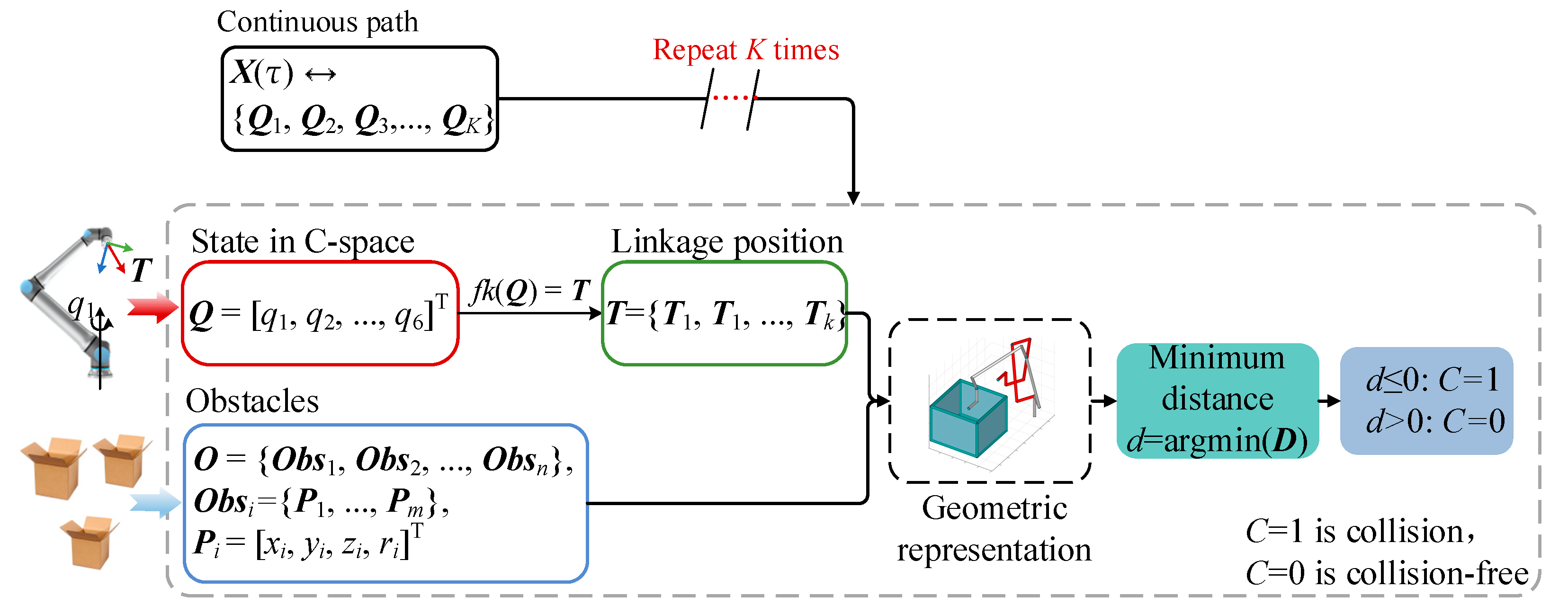
Traditional collision detection, as depicted in Figure 1, firstly maps joint positions Q to link positions T = {T1, …, Ti} by forward kinematics fk(∙), where i represents the link count. The links and obstacles are then represented using convex geometries such as capsules, spheres, and boxes. Obstacle information is described by the set O = {Obs1, Obs2, …, Obsj}, where each obstacle Obsj is characterized by the coordinates Pj and radius rj of m points. Subsequently, the distance d between these geometries is computed to determine the occurrence of collisions, which are classified as C. If d is not greater than 0, it is judged to be a collision, in which case C is defined as 1; otherwise, it is a non-collision state C = 0. For continuous path collision detection, the path X(τ) is discretized at a resolution K and detection is repeated for each sample point. This process is known as the exact collision detection method. Collision detection is transformed into the problem of computing the minimum distance between convex geometries.
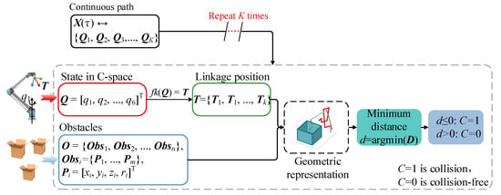
Figure 1.
The flow of exact collision detection.
There are numerous methods for calculating the Euclidean distance between two simple convex geometries. Mohammad Safeea et al. introduced an efficient approach to compute the minimum distance between capsules based on QR decomposition [13] and used it for the path planning of a robotic arm [14,15]. Reference [16] proposed a new calculation method of the distance between the sphere and the capsule and used it to detect the collision of the links of manipulators.
The problem of computing the distance between general convex geometries is more complicated. The Gilbert–Johnson–Keerthi (GJK) algorithm [17] and the Lin-Canny algorithm [18] are widely used. The GJK algorithm reduces the complexity of convex geometry by Minkowski distance, which has been widely used in computer graphics [19]. The swept volume intersection (SVI) method is suitable for detecting collisions along continuous paths [20]. It improves accuracy by assessing the collision situation based on the overlap rate. However, the calculation of the scanning volume of objects with complex geometry is very expensive [21]. The hierarchical bounding box (BVH) methods are proposed to enhance computing speed and memory optimization [22]. However, BVH methods may be too conservative in space, leading to inefficient exploration [23]. Exact collision detection algorithms have been well developed and most of them have been integrated in the flexible collision library (FCL) [24]. The exact collision detection methods ignore the correlation of states in C-space, which makes them time-consuming.
Learning-based methods provide an alternative strategy, which fits the obstacle manifolds in C-space to obtain information about the free configuration space (Cfree). Learning-based methods reduce the number of exact collision detections and significantly improve computational efficiency [25]. Pan et al. used incremental support vector machines (SVM) to learn an accurate model of the Cfree but the accuracy was not high and could not be applied to an unstructured environment [26]. Configuration space decomposition strategy can further improve the accuracy of collision detection methods based on SVM [27]. Huh attempts to fit the Cfree of a high-DOF manipulator using a Gaussian mixture model (GMM) but the fitting capability is limited [28]. Nikhil Das et al. proposed a collision detection model based on online learning, which is called Fastron [29]. Fastron learns the offline dataset based on Kernel Perceptron and obtains the optimal model to represent the boundary of the free configuration space within the maximum number of iterations [30]. A new kernel function is designed based on Fastron, which enhances the relationship between kinematics and configuration space and improves the accuracy of collision detection [31]. The DiffCo method is similar to Fastron in that obstacle manifold information is learned through a nonparametric kernel perceptron but it is mainly applied to optimization-based motion planners [32].
The above methods typically require the support of an offline dataset, making it difficult to transfer fitting capabilities to robots outside of the dataset. In addition, these methods are inapplicable for continuous path collision detections. Addressing these shortcomings, Pan Jia et al. proposed a K-nearest neighbors-based (KNN-based) collision classification method utilizing locality-sensitive hashing (LSH) for nearest neighbor queries and KNN for collision probability estimation [33]. The composite collision detection method (CCD) combined with the KNN method improves the accuracy in some special cases and can be applied to the RRT algorithm [34]. However, limited by the query efficiency, the computation speed of the KNN-based method is not maximized.
The KNN method, designed to identify the nearest neighbor information, has garnered significant attention across multiple domains, including databases [35,36], image processing [37], and deep learning-based control [38,39]. To reduce the complexity of the data search, practical implementations of KNN often employ approximate solutions. Among these, the graph-based KNN approach stands out as a prominent method for approximate querying [40]. The graph-based method constructs a neighborhood graph, where each data point corresponds to a node, the edges connecting the nodes define the neighborhood relationship, and the search speed is improved by the edges [41]. HNSW (hierarchical navigable small world) is a widely influential graph-based approximate KNN method [42]. HNSW is recognized as one of the most effective algorithms for querying speeds with fewer than 10,000 nearest neighbors and guarantees perfect recall [43]. KNN-based collision detection only needs to query a small number of nearest neighbors (less than 100) of the new node. Consequently, the HNSW algorithm is particularly well-suited to this task.
In this paper, a fast collision detection method is proposed to transform the collision detection into a binary classification problem. It incrementally constructs a collision database throughout the planning phase, queries this database for state information near the target using the HNSW method, and introduces an enhanced Gaussian probabilistic classifier for state classification. By leveraging local state correlations and circumventing the inefficiencies of exact collision detection, this method requires no training and facilitates collision detections on continuous paths. The primary contributions include the following:
- An incremental construction approach for a collision information database based on HNSW;
- A KNN query technique for linear data employing minimum threshold segmentation;
- A novel collision classifier, tailored to the kinematic characteristics of the manipulator.
The rest of the article is organized as follows. Section 2 introduces the HNSW algorithm and describes the KNN query way for point state and line state. Section 3 presents a new collision classifier based on the kinematic characteristics of the manipulator. Simulation experiments in Section 4 verify the superior performance of the proposed method. The conclusion is given in Section 5.
2. Construction of a Collision Database Based on HNSW
This section presents the technical details of KNN queries in the proposed approach. For ease of reading, a nomenclature table is provided in Abbreviation part, which records the variables and abbreviations in the following sections.
2.1. Introduction to HNSW
The goal of the KNN query is to find the k closest neighbors to the target. The HNSW (hierarchical navigable small world) method is a graph-based approximate nearest neighbor (ANN) search algorithm primarily employed for efficiently handling KNN queries in high-dimensional data. HNSW merges the characteristics of small-world networks with a hierarchical strategy, accelerating queries and insertion operations through a multi-layered graph structure. The database construction entails the following:
- Hierarchical structure: HNSW constructs a multi-layered graph, with each layer being a navigable graph. The bottom layer (level 0) contains all nodes, with higher layers progressively having fewer nodes. Each node, upon insertion, is randomly assigned a maximum layer, ensuring sparsity in higher layers;
- Node insertion: A new node is first located in the highest layer graph using a greedy search to find its nearest neighbors, then moves down layer by layer, performing a local greedy search at each level until reaching level 0. At each layer, the node selectively connects to other nodes in that layer based on distance criteria;
- Connection strategy: Each node maintains a limited-size list of its perceived nearest neighbors. This constrains each node’s out-degree, maintaining the graph’s sparsity while ensuring efficient search capability.
The KNN query process for a new node unfolds as follows:
- Initiating Search: Given a query point, the search begins at the highest layer, employing a greedy strategy to find the nearest neighbor at the current layer;
- Descending Through Layers: Once a local nearest neighbor is found at a current layer, the search moves to the next lower layer, continuing the search from this basis. This process is repeated down to level 0;
- Greedy Search: At each layer, the next closest node is greedily selected by comparing distances between the node and the query point until no closer node can be found.
This paper implemented HNSW by using the open-source code (https://github.com/nmslib/hnswlib, accessed on 6 April 2024.) and Euclidean distance as the metrics. The parameters in the HNSW algorithm all use the values suggested in reference [42].
2.2. Construction of Collision Database
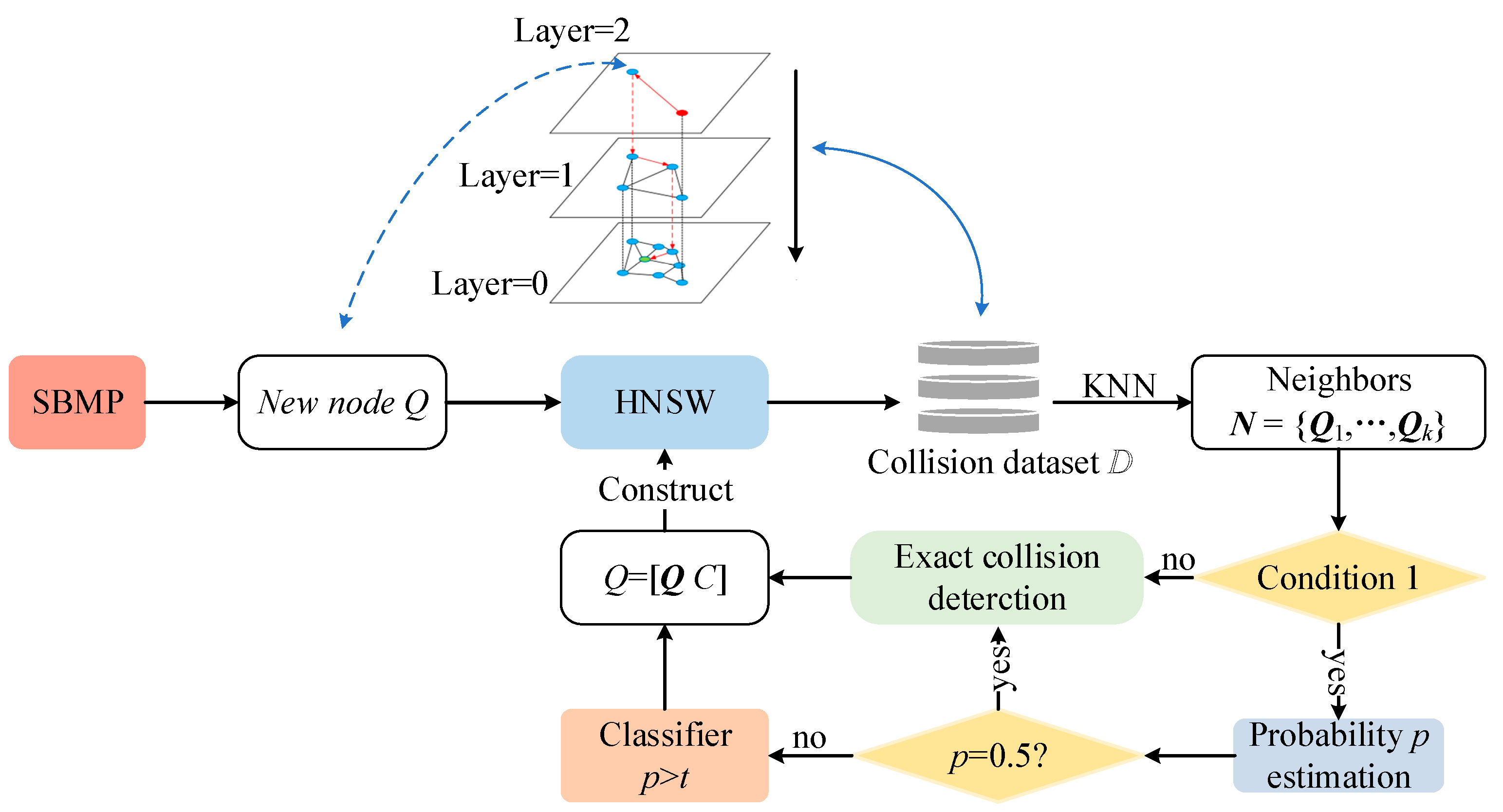
A node in C-space is defined by a set of joint angles, denoted as Q = [q1, q2, …, qn]. The database stores these nodes Q with an associated collision label C, where C can be either collision-free (C = 0) or collision (C = 1). Using the HNSW method, we incrementally construct the collision database as shown in Figure 2.
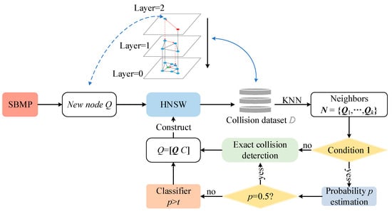
Figure 2.
The construction process of the collision database.
As depicted in Figure 2, the planner initially obtains Q through random sampling in C-space, then uses HNSW to search for the k-nearest neighbors set N of Q. Condition 1 is introduced here to exclude nodes that are significantly distant from other nodes, as their collision probability is hard to estimable based on neighboring information.
Condition 1.
The number of neighbors satisfies
. A neighbor is a node whose distance from the new target is at most a threshold Dd, where Dd = 0.1·Scale, and Scale is the size of the database.
When Condition 1 is satisfied, the collision probability p of Q is estimated. If p satisfies Condition 2, the collision label C is determined by comparing p with the threshold t; C = 1 if p > t and C = 0 otherwise. The value of t will affect the accuracy of classification and it is suggested to be 0.2 to 0.5 in this paper. If Condition 1 is not satisfied, the label C of Q is obtained by exact collision detection and the node [Q C] is added to the database.
Condition 2.
The collision probability p of a node is not equal to 0.5. The reason for rejecting the classification of nodes with p = 0.5 is that these nodes are on the edge of the obstacle manifold and it is difficult for the classifier to accurately decide the collision category.
In summary, when both Conditions 1 and 2 are satisfied, the classification is completed by the collision probability of Q; otherwise, exact collision detection is performed on Q. After obtaining the collision label C, Q is added to the collision database.
2.3. KNN Query Method for Line Data Based on Threshold Segmentation
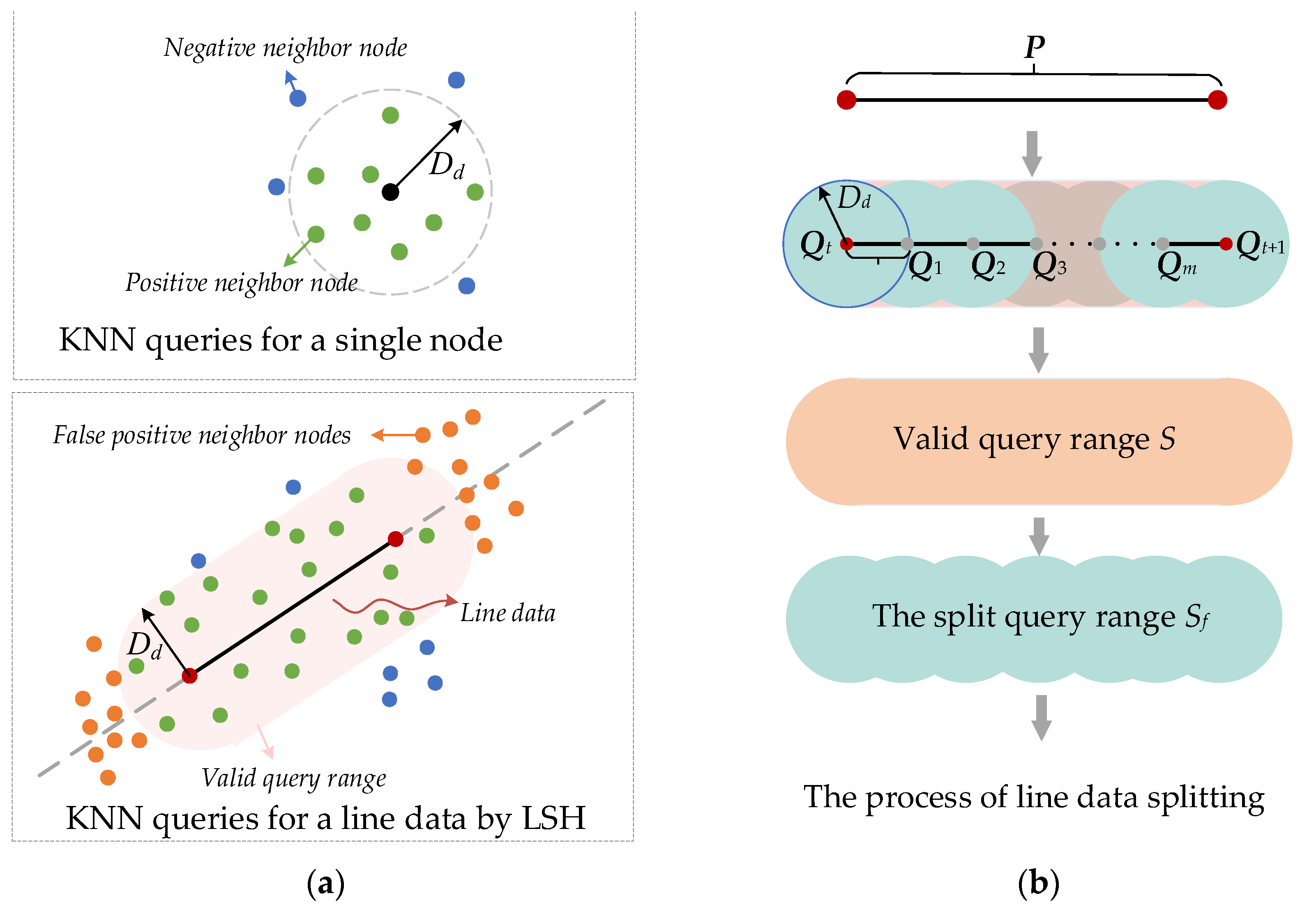
Line data P = [Qt, Qt+1] representing manipulator motion from Qt to Qt+1 pose a greater collision detection frequency in SBMP than single nodes. The dimensions of nodes Q and P cannot be aligned, so it is difficult to directly use the method shown in Figure 2 to perform KNN queries on P. In reference [33], a method of augmenting vectors was proposed to make Q and P have the same dimension, denoted as the LSH method. However, LSH complicates computations and risks false positives by treating line data as straight lines, as illustrated in Figure 3a.
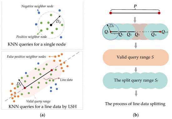
Figure 3.
KNN query process of the LSH method and the proposed method. (a) KNN queries for a single node and line data by LSH-based. (b) KNN query process for line data based on the proposed method.
To address these issues, we introduce a threshold segmentation-based method, where Dd segments line data into a set D of points, reducing computational complexity and minimizing false positives, as defined in Equation (1).
where n is the number of split points, m = g(norm(P)/Dd), the norm( ) computes the length of a vector, and the g( ) is the rounding function.
The Qi is calculated by Equation (2), where v is the unit vector of P.
The elements in D are then traversed to obtain the neighbors and the union of the neighbors of all elements is the neighborhood of the line data.
Since the range Sf of the segmented query is smaller than the valid range S, the proposed method will lose a small number of positive neighbor nodes of line data, as shown in Figure 3b. The upper bound of the probability of the loss can be obtained from Equation (3). Despite a potential loss of positive neighbors due to smaller query ranges, this method’s impact on collision detection accuracy is negligible, making it an acceptable compromise.
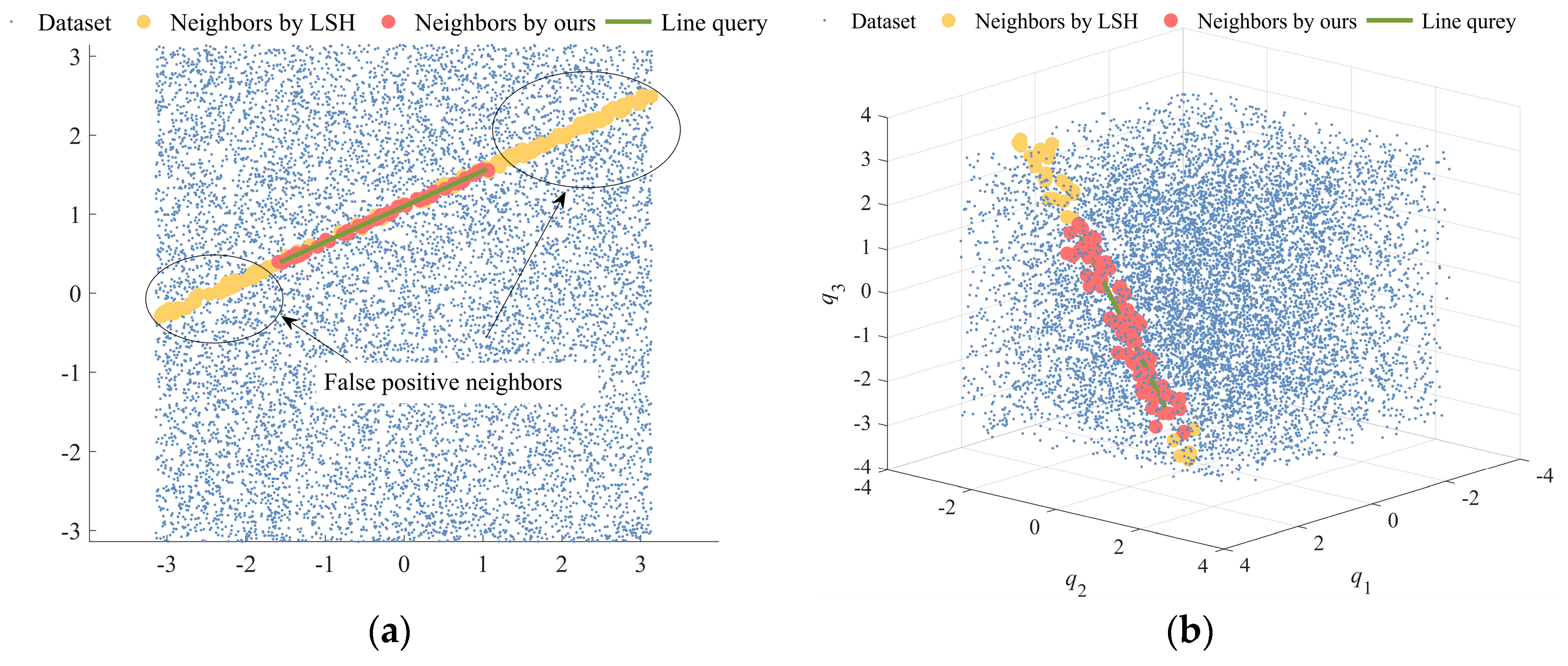
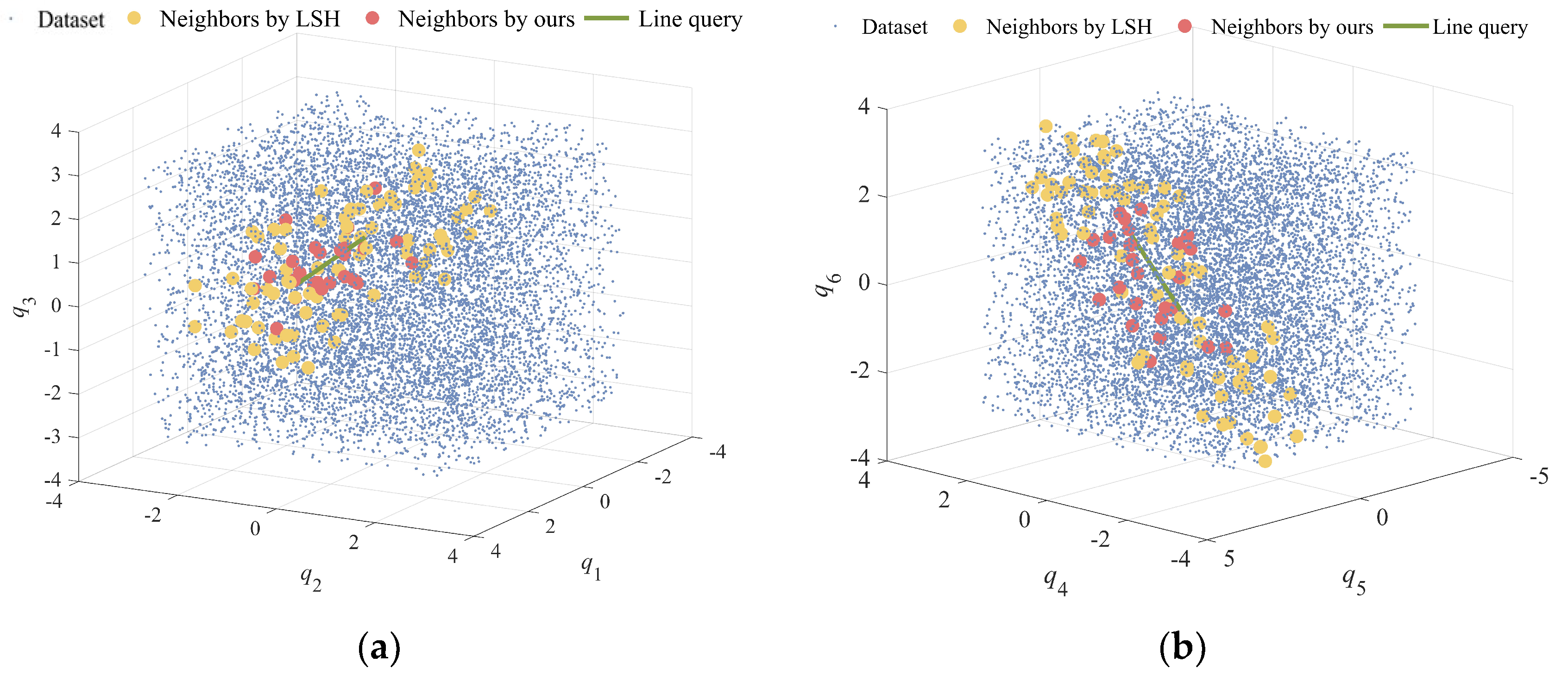
In the range [−π, π], 10,000 sets of 2D, 3D, and 6D nodes are randomly selected as the database to test the performance of the LSH method and the proposed method. Figure 4 illustrates the query results for the 2D and 3D databases, with red dots representing queries by the proposed method and yellow dots indicating those by the LSH method. The proposed method demonstrated a notable reduction in false positives, a trend consistent across the 6D database as well, as presented in Figure 5. This indicates the proposed method’s superior accuracy in filtering relevant data across multiple dimensions.
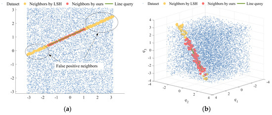
Figure 4.
Query results for both methods in 2D and 3D databases. (a) Query results of both methods in the 2D database. (b) Query results of both methods in the 2D database.

Figure 5.
Query results for both methods in 6D databases. (a) Visualization of the first 3D query results for 6D data and (b) visualization of post-3D query results on 6D data.
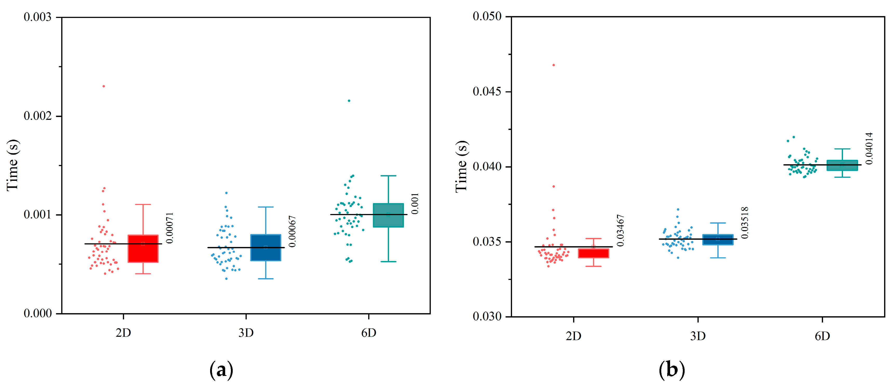
KNN queries are performed on 50 different sets of continuous paths on three datasets. To fairly compare the performance of the two methods, brute-force query is used in both retrieval methods; the final time performance of the two methods in the continuous path scene is shown in Figure 6a, which shows the query time of the proposed method in the three datasets.

Figure 6.
Comparison of the query time between the two methods in the three datasets. (a) Time performance of the proposed method on three datasets and (b) time performance of the LSH method on three datasets.
The proposed method exhibits superior efficiency in query times compared to the LSH method across datasets of varying dimensions. Specifically, the average query times for the proposed method are 7.1 × 10⁻⁴ s for 2D, 6.7 × 10⁻⁴ s for 3D, and 1.0 × 10⁻³ s for 6D datasets, as recorded in Figure 6a. In contrast, the LSH method shows average query times of 3.46 × 10⁻², 3.52 × 10⁻², and 4.01 × 10⁻² s for 2D, 3D, and 6D datasets, respectively, as indicated in Figure 6b. Thus, the proposed method achieves a query time efficiency improvement by two orders of magnitude for 2D and 3D datasets and a 97.5% reduction for 6D datasets. These simulation results underscore the proposed method’s significant time-saving advantage over the LSH approach.
In summary, the proposed method offers three key benefits in KNN queries of line data over the LSH method:
- (1)
- Lower Memory Requirement: It maintains the original database vector form without needing extra memory for storing augmented vectors;
- (2)
- Elimination of Post-Processing: By segmenting line data and querying neighbor data within each segment’s maximum range, it circumvents the need to filter out false positives, a step required by the LSH method;
- (3)
- Reduced Time Consumption: Utilizing the Euclidean distance for queries in the d-dimensional database minimizes computational complexity relative to the LSH’s augmented vector approach.
3. Design of Collision Classifier
It is considered that within a reasonable range of Dd, the node under test has a probability consistency with its neighbor set. Therefore, the collision probability P can be estimated according to the collision situation of neighboring nodes and the type of collision can be judged by P. Based on this theory, we design a new collision classifier.
Firstly, we use a Gaussian function to weigh the influence of neighbors at different distances and the weights are defined by Equation (4).
where Q is the target node or a line data, xi is the ith neighbor data, ρ() is the distance function, and γ is the weight controlling the scale, which is calculated by Equation (5).
As the distance between the neighbor node and the node or line data to be tested decreases, the probability of the two collision types being the same increases. The distance function ρ() is used to calculate the similarity of state variables, which is crucial for collision type estimation. Each joint has different effects on the movement of the link and the way to calculate the node distance will lead to changes in the motion configuration of the manipulator [44]. The influence of different joints is assigned by weights and the distance function is defined as
where ΔQ is the joint distance vector and M is a diagonal matrix whose elements are joint weights. M can be customized by users; this paper suggests diag(0.32, 0.27, 0.23, 0.05, 0.2, and 0.05). The collision probability of node Q is estimated by Equation (7).
where N is the set of neighbors and the sigmoid function is used to improve the sensitivity of the classifier. Here, μ1 and μ2 are the mean values of the Gaussian distribution and σ12 and σ1 are the variances of the Gaussian distribution [45], which can be obtained from Equations (8) and (9), respectively. The parameter ci is the collision state of xi and the value is 0 or 1.
To classify a node’s collision state, a threshold t ~ (0, 1) is applied. If P[c(Q) = 1|D] > t, Q is deemed colliding; otherwise, it is collision-free. A threshold of 0.2 is empirically chosen. For line data, the collision probability calculation differs and is outlined in a distinct equation, as shown in Equation (10).
where the function Near(P, x) returns the point closest to x on P. The other variables are calculated by Equations (8) and (9) but it should be noted that the variables in the weighted distance function need to be changed to line data P.
The collision state of P is predicted using a similar threshold strategy, with t = 0.25 for line data, to determine whether the line segment is colliding or collision-free. This methodology underscores a systematic approach to estimating collision probabilities and classifying collision states for both nodes and line data, leveraging the relational dynamics within a node’s neighbor set.
4. Simulation and Results
4.1. Introduction to the Obstacle Environment and Databases
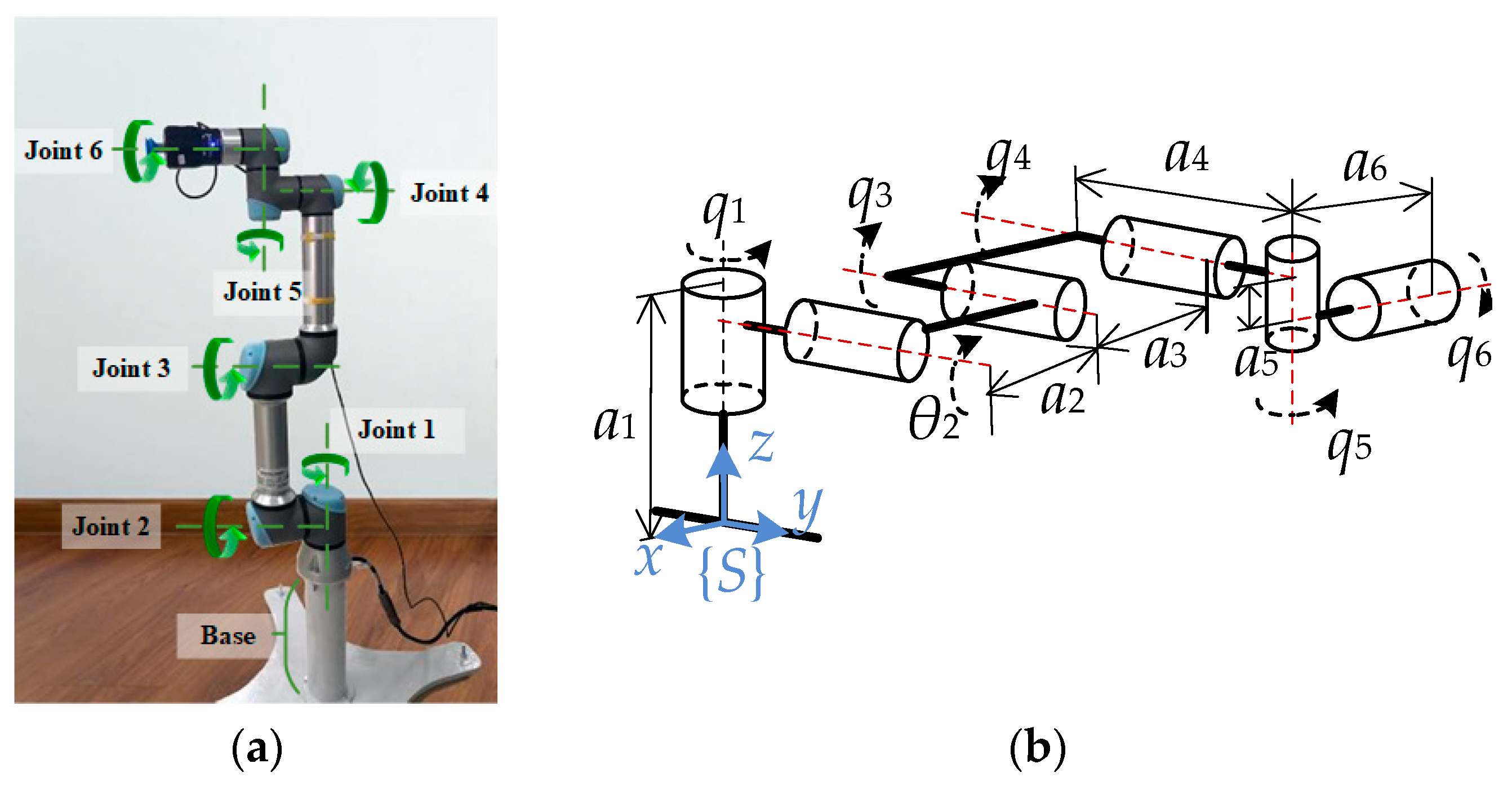
In this paper, the UR5 robot is used as the simulation object, as shown in Figure 7, where ai is the length of the connecting rod and qi is the rotation angle of the i-th joint. The axes of adjacent joints are orthogonal or parallel.
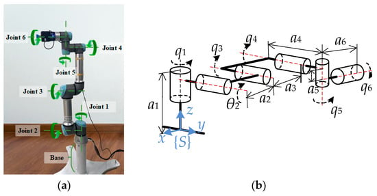
Figure 7.
Structure diagram of UR5. (a) UR5 manipulator and (b) Structure diagram of UR5, a1 = 780 mm, a2 = 320 mm, a3 = 1125 mm, a4 = 200 mm, a5 = 1142.5 mm, and a6 = 82.5 mm.
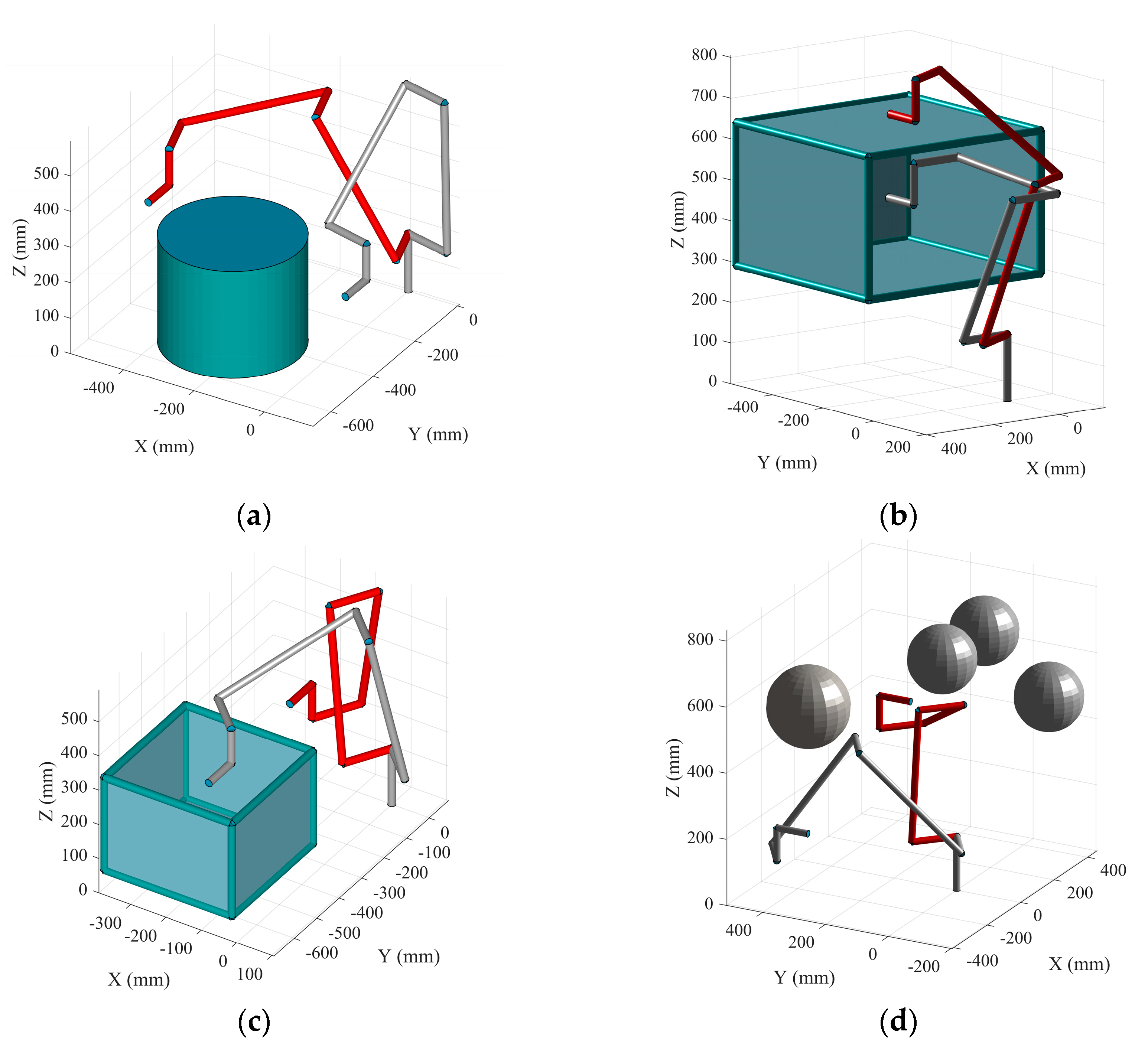
Four obstacle environments were simulated and designed, which were defined as cylinder scene, drawer scene, box scene, and sphere scene, respectively, as shown in Figure 8. The capsules are used to represent the linkage of the UR5 robot and obstacles are composed of spheres, capsules, and planes. The experiments were performed on an IntelⓇ CoreTM i7-9750H, @2.60GHz CPU.

Figure 8.
Simulation environments for the four different obstacles. (a) Cylindrical obstacle scene; (b) Drawer obstruction scene; (c) Box obstacle scene; and (d) Sphere obstacle scene.
The cylinder scene has only one obstacle, the drawer scene and the box scene have 17 obstacles, including 12 capsules and 5 planes, and the sphere scene has 4 sphere obstacles. The database is composed of 30,000 sets of random sampling nodes in the configuration space and the data form is Q = [q1, q2,..., q6, c]. The ratio of positive samples to negative samples was 1:3. The test set is divided into two categories, 1000 discrete nodes Qs, and 1000 continuous path Ps. We use FCL to obtain the real collision situation of all the data.
Accuracy (Ac), specificity (TNR), and sensitivity (TPR) were used to measure the performance of the algorithm. Ac was the prediction accuracy rate, TPR was the proportion of samples correctly classified in collisions, and TNR was the proportion of samples correctly classified without collisions. The three metrics are defined in Equation (11).
where TP is the number of true positive samples, TN is the number of true negative samples, FP is the number of false positive samples, and FN is the number of false negative samples.
We use three methods for collision detection of test sets, namely the Fastron method [29], the LSH method [33], and the proposed method. The three algorithms are implemented at the same hardware level and the specific parameters of Fastron and LSH algorithms are detailed in their references.
4.2. Collision Detection of a Single Node
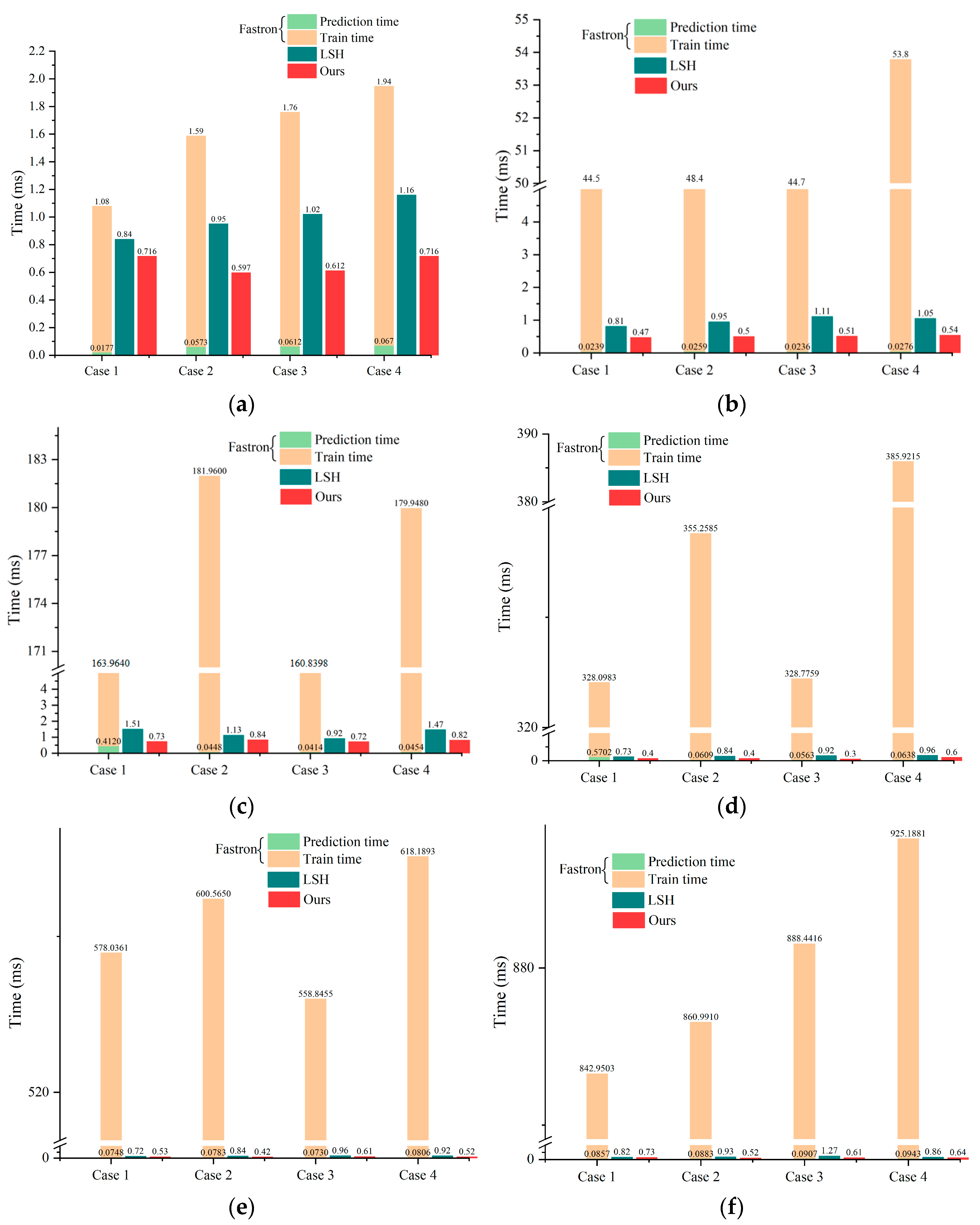
In examining the average detection times across four distinct scenarios, as delineated in Figure 9, it is observed that the Fastron method significantly outpaces the LSH and proposed methods in prediction speed, achieving microsecond-level efficiency. Nonetheless, this advantage is mitigated by the additional temporal expenditure required for Fastron’s training phase, which escalates exponentially with the augmentation of the training set size, ranging from 1 ms to 900 ms. Consequently, the ostensibly superior speed of Fastron is counterbalanced by its extensive training duration, eroding its overall temporal advantage.
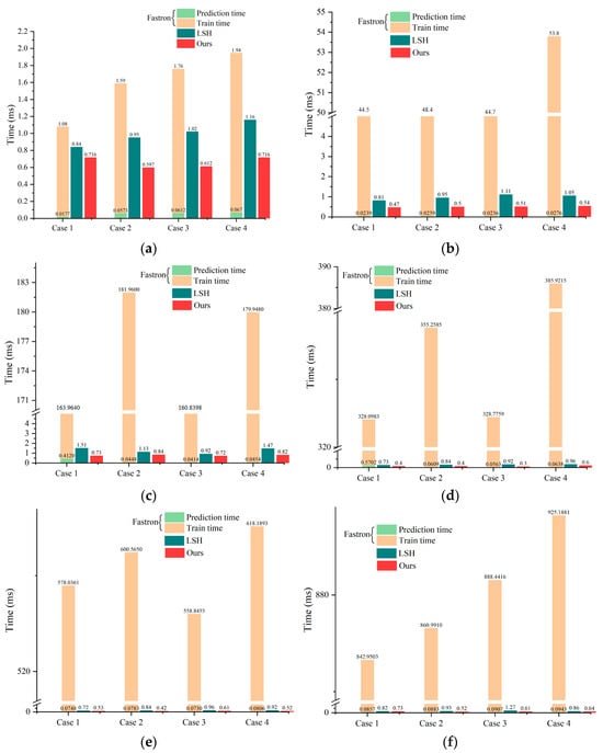
Figure 9.
Time performance of Fastron, LSH, and our methods on different training sets. (a) Size = 1000; (b) Size = 5000; (c) Size = 10,000; (d) Size = 15,000; (e) Size = 20,000; and (f) Size = 25,000.
The comparative analysis presented in Figure 9a–f highlights the performance enhancements afforded by the proposed method over the LSH method across varying training set sizes. Specifically, with a training set size of 1000, the proposed method exhibited improvements in prediction speed by 14.8%, 37.2%, 40.0%, and 38.3% across the four simulated environments. Incremental increases in training set size to 5000; 10,000; 15,000; 20,000; and 25,000 further amplified the proposed method’s performance advantage, with respective speed enhancements of 23.0%, 47.4%, 54.1%, 48.6%; 51.7%, 25.7%, 13.7%, 44.2%; 18.2%, 36.4%, 58.7%, 33.5%; 26.4%, 34.0%, 32.5%, and 43.5% and finally, 10.8%, 44.1%, 52.0%, and 25.6%.
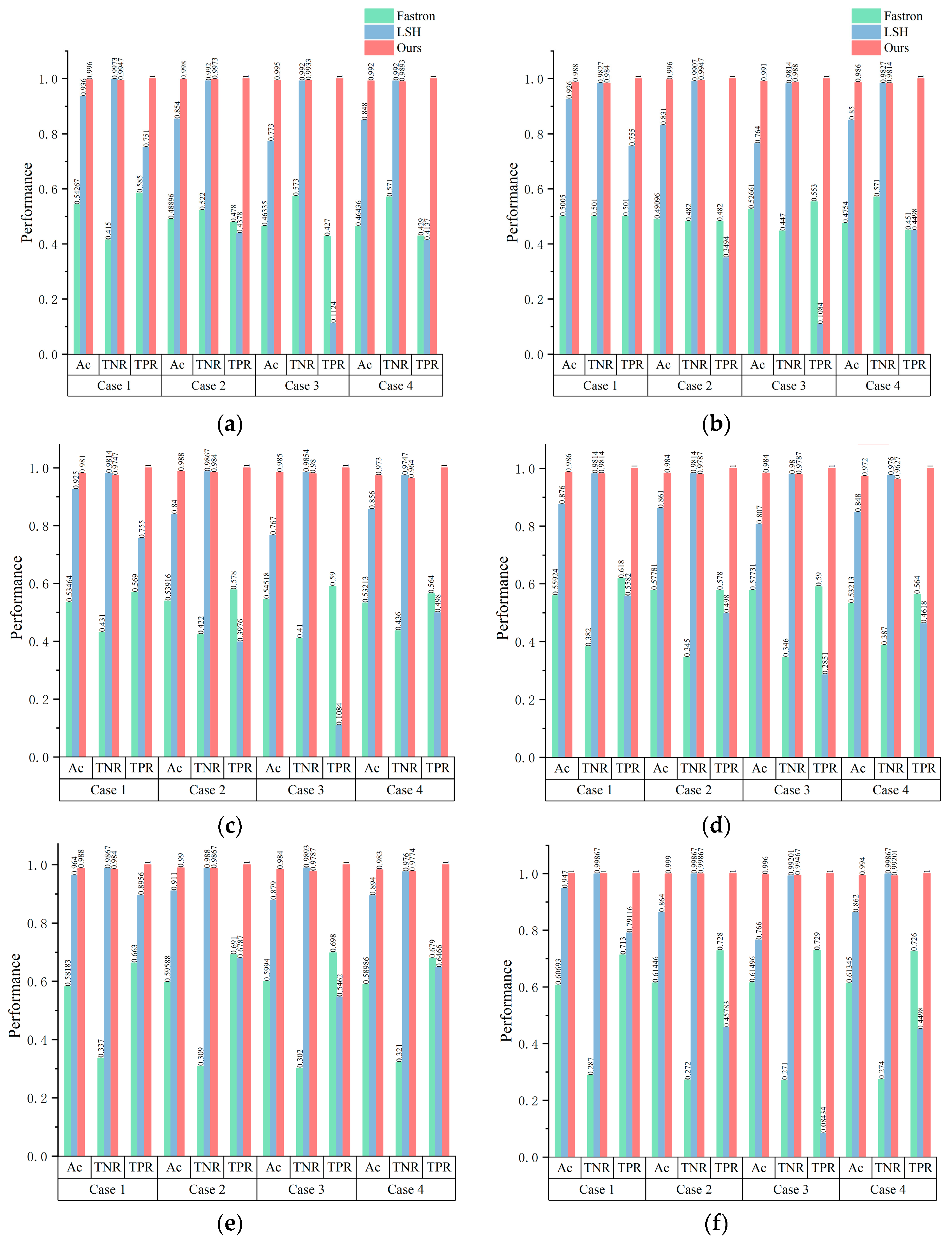
Disregarding the duration necessary for training, the Fastron method distinctly leads in detection time, surpassing the other two methodologies by approximately an order of magnitude. Nevertheless, the LSH and the proposed methods have their inherent advantages, chiefly their non-reliance on a training phase. Furthermore, the proposed method benefits from a hierarchical design, ensuring that the time required for nearest neighbor retrieval via HNSW remains stable irrespective of increases in the training set size. Figure 10a–f shows the performance of the three methods on the three metrics. Obviously, the proposed method performs best in four scenes with training samples of different sizes.
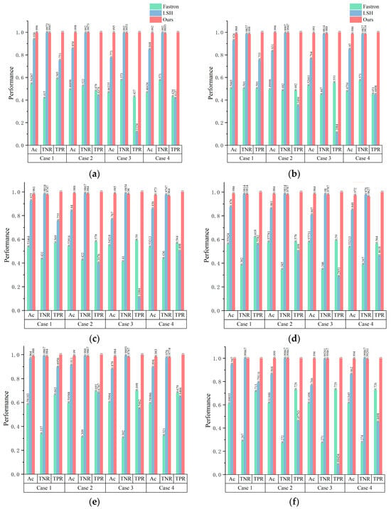
Figure 10.
The Ac, TNR, and TPR performances of Fastron, LSH, and our methods on training sets of different sizes. (a) Size = 1000; (b) Size = 5000; (c) Size = 10,000; (d) Size = 15,000; (e) Size = 20,000; and (f) Size = 25,000.
Figure 10a delineates that, with a sample size of 1000, the Fastron method’s accuracy falls below 50% across all but one scenario, suggesting its limitations in complex environments with minimal training data. Conversely, the method proposed herein achieves significantly higher accuracy rates-surpassing the LSH method by margins of 6.0%, 16.9%, 28.7%, and 17.0% across the four evaluated scenes. This discrepancy highlights the proposed method’s superior ability to correctly identify collision instances.
As the sample size escalates to the range of 5000 to 20,000, the Fastron method shows an uptick in detection accuracy, surpassing 50% in all scenarios and occasionally exceeding 60%. However, these figures, while improved, remain modest. During this expansion, the relative performance gap between the LSH and proposed methods widens, with the latter maintaining an exceedingly high accuracy level of over 98% across all scenarios and sample sizes, underscoring its robustness and adaptability.
Upon further increasing the sample size to 25,000, the LSH method experiences a notable decline in detection accuracy. This reduction is attributed to the method’s susceptibility to the effective range or k-value parameter, complicating the extraction of obstacle features and causing positive sample neighbors to erroneously influence classification outcomes. The distance function introduced by the proposed methodology effectively mitigates such interference, sustaining remarkable accuracy levels of 100%, 99.9%, 99.6%, and 99.4% across the four scenes. This performance underscores the proposed method’s capacity to provide reliable collision detection in robotic path planning.
4.3. Collision Detection of Continuous Paths
According to the above analysis, it can be seen that the performance of the Fastron method in a complex environment is not ideal. Therefore, Fastron is excluded from the comparison. To ensure a balance between computational efficiency and detection accuracy, a training set with a fixed size of 2000 samples was employed, with a sampling frequency of 500 for precise collision detection along continuous paths.
Table 1 presents the execution times for exact collision detection, LSH-based methods, and the proposed method across four distinct environments. The recorded times for the LSH-based method reflect only correctly predicted samples to mitigate the distortion from anomalous samples on the analysis’s integrity.

Table 1.
Execution time in four environments for exact collision detection, the LSH method, and our method (ms).
The data reveal that the proposed method outperforms the exact collision detection and LSH methods in terms of speed, boasting improvements of 96.6% and 79.5% in Scene 1, 97.0% and 72.4% in Scene 2, 98.2% and 80.6% in Scene 3, and 98.4% and 76.1% in Scene 4, respectively. These findings underscore the proposed method’s significant efficiency across all evaluated environments.
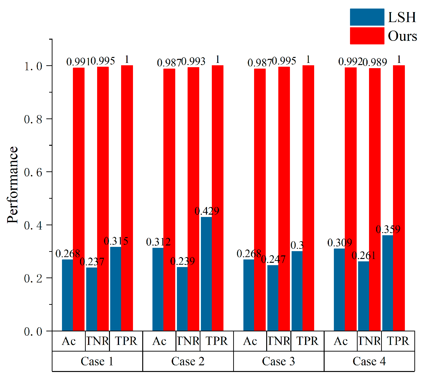
Furthermore, as illustrated in Figure 11, the proposed method demonstrates consistently high accuracy in detecting collisions along continuous paths, with accuracies of 99.1%, 98.7%, 98.7%, and 98.2% in the four scenarios, respectively. The true positive rate (TPR) confirms the proposed method’s reliability in accurately identifying collisions. Conversely, the LSH method’s performance is markedly impaired by irrelevant samples, leading to significantly reduced accuracies of 26.8%, 31.2%, 26.8%, and 30.9%, with true negative rates (TNR) of 23.7%, 23.9%, and 26.1%, respectively.
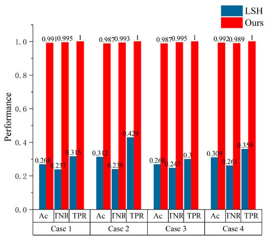
Figure 11.
Ac, TNR, and TPR performance of the continuous paths of the LSH and our method in the four cases.
Simulation results show that the performance of the proposed method for continuous path detection (Ac, TNR, and TPR) is much better than that of the LSH method in four scenarios. In the detection of continuous paths, our method still maintains the same detection speed advantage as the discrete configuration sample, which is attributed to the method in Section 2.3. In addition, compared with the LSH method, the HNSW method has advantages in KNN queries.
4.4. Collision Detection for Manipulators with Different Degrees of Freedom
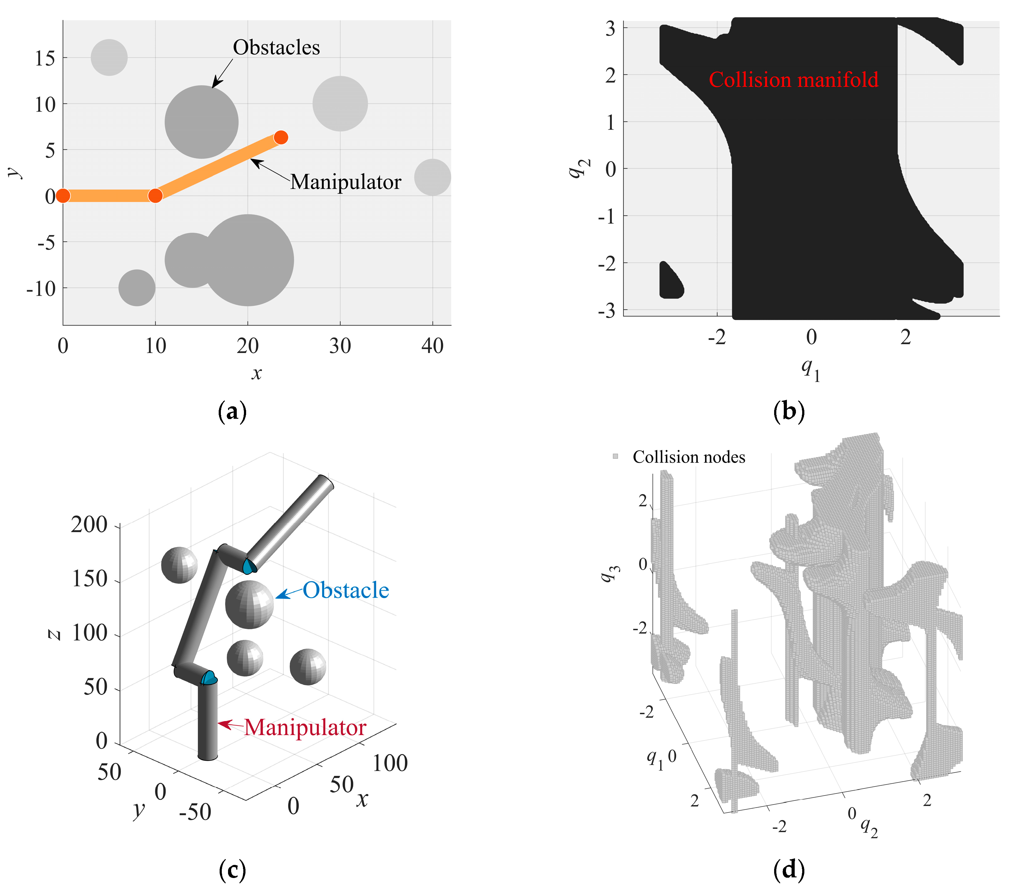
To evaluate the proposed method’s performance across manipulators with varying degrees of freedom (DOF), we conducted simulations on 2DOF and 3DOF manipulator systems. The obstacles and their associated collision manifolds for both manipulators are depicted in Figure 12.
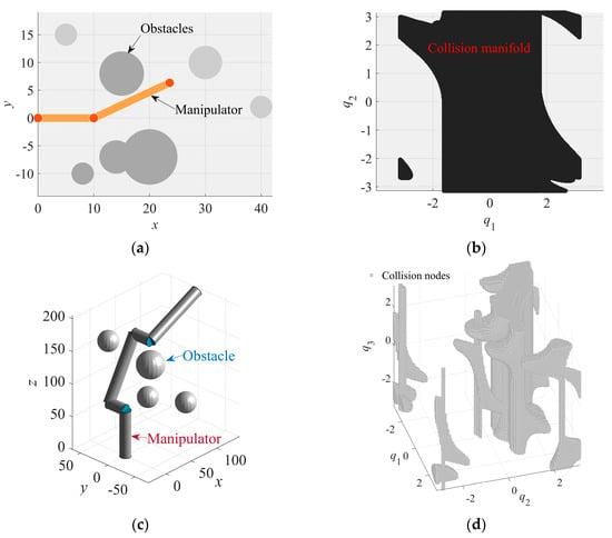
Figure 12.
Obstacle environments and corresponding collision manifolds for the two manipulators. (a) Obstacle environment for a 2DOF manipulator; (b) Collision manifold for the 2DOF manipulator; (c) Obstacle environment for a 3DOF manipulator; and (d) Collision manifold for the 3DOF manipulator.
Initially, 10,000 random nodes are sampled within the configuration space of each manipulator; the FCL is utilized to ascertain the true collision status of each node. Subsequently, a subset of 5000 samples was selected as the test set to assess the accuracy (Ac) and execution time of both the proposed method and the LSH method, with the comparative results detailed in Table 2.

Table 2.
The Ac and execution time of the LSH method and our method on the two manipulators.
Table 2 demonstrates that the LSH and the proposed method both exhibit high accuracy in collision detection for the 2DOF manipulator, achieving 94.47% and 99.57% accuracy, respectively. Our method not only improves accuracy by 5% but also reduces the computation time by 33.50%. For the 3DOF manipulator’s collision detection, the proposed method’s time efficiency is even more pronounced, yielding a 62.65% time reduction compared to the LSH method while simultaneously increasing accuracy by 9.6%.
The above results show that the proposed method consistently delivers high accuracy and speed across manipulators with varying DOF, substantiating its robustness and efficiency in diverse robotic configurations.
5. Conclusions
This paper presents a rapid collision detection method based on probability classification, which can be used for collision detection of continuous paths. The proposed method constructs the collision database incrementally and the KNN query is performed on the target based on the HNSW method. Moreover, the challenge of continuous path KNN query is solved by adopting a threshold segmentation strategy, which effectively reduces the influence of irrelevant samples, thus improving the efficiency and accuracy of the query. Finally, the collision state classifier based on the weighted distance function is used to calculate the collision probability of the target state and complete the collision detection. Simulation results verify the effectiveness of the proposed method. Extending the proposed method to dynamic environments is a future work.
Author Contributions
Conceptualization and methodology, X.Z.; experiment, X.Z. and D.J.; writing—original draft preparation, X.Z.; supervision, B.T. and D.J.; review and editing, X.L.; funding acquisition, B.C., D.T. and B.T. All authors have read and agreed to the published version of the manuscript.
Funding
This work was supported by grants of the National Natural Science Foundation of China (Grant Nos. 51975324, 51505349); Open Fund of Hubei Key Laboratory of Hydroelectric Machinery Design and Maintenance in China Three Gorges University (2020KJX02, 2021KJX13); and Science and Technology Planning Project of Inner Mongolia Autonomous Region (No. 2020GG0105).
Data Availability Statement
The data presented in this study are available on request from the corresponding author.
Conflicts of Interest
The authors declare no conflicts of interest.
Abbreviations
| Nomenclature | Definition |
| SBMP | Sampling-based motion planner |
| C-space | Confugration space |
| Cfree | Collision-free confugration space |
| KNN | K-nearest neighbors |
| ANN | Approximate nearest neighbor |
| FCL | Flexible collision library |
| LSH | Locality-sensitive hashing method |
| HNSW | Hierarchical navigable small world |
| Ac | Accuracy |
| TNR | Specificity rates |
| TPR | Sensitivity rates |
| X(τ) | Continuous path in C-space |
| τ | Path parameter |
| Q | Confugration or node |
| T | Pose matrix |
| O | Set of obstacles |
| N | The set of neighbors of a node |
| P | Position vector |
| Obs | Pose matrix of obstacles |
| M | Distance weighted matrix |
| fk(∙) | Forward kinematics |
| ρ(∙) | The distance function |
| qi | The ith joint angle |
| C | Collision label |
| r | Radius |
| d | Minimum distance between envelopes |
| p | The collision probability of a node |
| Dd | Minimum distance threshold |
| t | Collision probability threshold |
References
- Park, K.M.; Park, Y.; Yoon, S.; Park, F.C. Collision detection for robot manipulators using unsupervised anomaly detection algorithms. IEEE/ASME Trans. Mech. 2022, 27, 2841–2851. [Google Scholar] [CrossRef]
- Liu, B.; Fu, W.; Wang, W.; Li, R.; Gao, Z.; Peng, L.; Du, H. Cobot motion planning algorithm for ensuring human safety based on behavioral dynamics. Sensors 2022, 22, 4376. [Google Scholar] [CrossRef]
- Zhang, X.; Li, G.; Xiao, F.; Jiang, D.; Tao, B.; Kong, J.; Jiang, G.; Liu, Y. An inverse kinematics framework of mobile manipulator based on unique domain constraint. Mech. Mach. Theory 2023, 183, 105273. [Google Scholar] [CrossRef]
- Zhu, H.; Ding, Y. Optimized dynamic collision avoidance algorithm for USV path planning. Sensors 2023, 23, 4567. [Google Scholar] [CrossRef]
- Geng, S.; Wang, Q.; Xie, L.; Xu, C.; Cao, Y.; Gao, F. Robo-Centric ESDF: A fast and accurate whole-body collision evaluation tool for any-shape robotic planning. In Proceedings of the IEEE/RSJ International Conference on Intelligent Robots and Systems (IROS), Detroit, MI, USA, 1–5 October 2023; pp. 290–297. [Google Scholar] [CrossRef]
- Han, F.; Gao, F.; Zhou, B.; Shen, S. FIESTA: Fast Incremental euclidean distance fields for online motion planning of aerial robots. In Proceedings of the IEEE/RSJ International Conference on Intelligent Robots and Systems (IROS), Macau, China, 3–8 November 2019; pp. 4423–4430. [Google Scholar] [CrossRef]
- Nayak, S.; Otte, M.W. Bidirectional sampling-based motion planning without two-point boundary value solution. IEEE Trans. Robot. 2022, 38, 3636–3654. [Google Scholar] [CrossRef]
- Palmieri, L.; Bruns, L.; Meurer, M.; Arras, K.O. Dispertio: Optimal sampling for safe deterministic motion planning. IEEE Robot. Autom. Lett. 2019, 5, 362–368. [Google Scholar] [CrossRef]
- Chen, G.; Luo, N.; Liu, D.; Zhao, Z.; Liang, C. Path planning for manipulators based on an improved probabilistic roadmap method. Robot. Comput. Manuf. 2021, 72, 102196. [Google Scholar] [CrossRef]
- Xu, J.; Song, K.; Zhang, D.; Dong, H.; Yan, Y.; Meng, Q. Informed anytime fast marching tree for asymptotically optimal motion planning. IEEE Trans. Ind. Electron. 2020, 68, 5068–5077. [Google Scholar] [CrossRef]
- Karaman, S.; Frazzoli, E. Sampling-based algorithms for optimal motion planning. Int. J. Robot. Res. 2011, 30, 846–894. [Google Scholar] [CrossRef]
- Liu, B.; Jiang, G.; Zhao, F.; Mei, X. Collision-Free Motion Generation Based on Stochastic Optimization and Composite Signed Distance Field Networks of Articulated Robot. IEEE Robot. Autom. Let. 2023, 8, 7082–7089. [Google Scholar] [CrossRef]
- Safeea, M.; Neto, P.; Bearee, R. Efficient calculation of minimum distance between capsules and its use in robotics. IEEE Access 2018, 7, 5368–5373. [Google Scholar] [CrossRef]
- Safeea, M.; Neto, P.; Bearee, R. On-line collision avoidance for collaborative robot manipulators by adjusting off-line generated paths: An industrial use case. Robot. Auton. Syst. 2019, 119, 278–288. [Google Scholar] [CrossRef]
- Safeea, M.; Neto, P. Minimum distance calculation using laser scanner and IMUs for safe human-robot interaction. Robot. Comput.-Int. Manuf. 2019, 58, 33–42. [Google Scholar] [CrossRef]
- Jiang, L.; Liu, S.; Cui, Y.; Jiang, H. Path planning for robotic manipulator in complex multi-obstacle environment based on improved_RRT. IEEE/ASME Trans. Mechatron. 2022, 27, 4774–4785. [Google Scholar] [CrossRef]
- Gilbert, E.; Johnson, D.; Keerthi, S. A fast procedure for computing the distance between complex objects in three-dimensional space. IEEE J. Robot. Auto. 1988, 4, 193–203. [Google Scholar] [CrossRef]
- Xu, J.; Liu, Z.; Yang, C.; Li, L.; Pei, Y. A pseudo-distance algorithm for collision detection of manipulators using convex-plane-polygons-based representation. Robot. Comput.-Int. Manuf. 2020, 66, 101993. [Google Scholar] [CrossRef]
- Montanari, M.; Petrinic, N.; Barbieri, E. Improving the GJK algorithm for faster and more reliable distance queries between convex objects. ACM Trans. Graph. 2017, 36, 1–17. [Google Scholar] [CrossRef]
- Li, D.; Zhang, J.; Liu, G. Autonomous driving decision algorithm for complex multi-vehicle interactions: An efficient approach based on global sorting and local Ggaming. IEEE Trans. Intell. Transp. Syst. 2024. [Google Scholar] [CrossRef]
- Ferguson, Z.; Li, M.; Schneider, T.; Gil-Ureta, F.; Langlois, T.; Jiang, C.; Zorin, D.; Kaufman, D.M.; Panozzo, D. Intersection-free rigid body dynamics. ACM Trans. Graph. 2021, 40, 338–353. [Google Scholar] [CrossRef]
- Ströter, D.; Mueller-Roemer, J.S.; Stork, A.; Fellner, D.W. OLBVH: Octree linear bounding volume hierarchy for volumetric meshes. Vis. Comput. 2020, 36, 2327–2340. [Google Scholar] [CrossRef]
- Wang, Q.; Wang, Z.; Pei, L.; Xu, C.; Gao, F. A linear and exact algorithm for whole-body collision evaluation via scale optimization. In Proceedings of the IEEE International Conference on Robotics and Automation (ICRA), London, UK, 29 May–2 June 2023; pp. 3621–3627. [Google Scholar] [CrossRef]
- Pan, J.; Chitta, S.; Manocha, D. FCL: A general purpose library for collision and proximity queries. In Proceedings of the IEEE International Conference on Robotics and Automation (ICRA), Saint Paul, MN, USA, 14–18 May 2012; pp. 3859–3866. [Google Scholar] [CrossRef]
- Qureshi, A.H.; Miao, Y.; Simeonov, A.; Yip, M.C. Motion planning networks: Bridging the gap between learning-based and classical motion planners. IEEE Trans. Robot. 2020, 37, 48–66. [Google Scholar] [CrossRef]
- Pan, J.; Manocha, D. GPU-based parallel collision detection for fast motion planning. Int. J. Robot. Res. 2012, 31, 187–200. [Google Scholar] [CrossRef]
- Han, Y.; Zhao, W.; Pan, J.; Liu, Y.-J. Configuration space decomposition for learning-based collision checking in high-DOF robots. In Proceedings of the IEEE/RSJ International Conference on Intelligent Robots and Systems (IROS), Las Vegas, NV, USA, 25–29 October 2020; pp. 5678–5684. [Google Scholar] [CrossRef]
- Huh, J.; Lee, B.; Lee, D.D. Adaptive motion planning with high-dimensional mixture models. In Proceedings of the IEEE International Conference on Robotics and Automation (ICRA), Singapore, 29 May–3 June 2017; pp. 3740–3747. [Google Scholar] [CrossRef]
- Das, N.; Yip, M. Learning-based proxy collision detection for robot motion planning applications. IEEE Trans. Robot. 2020, 36, 1096–1114. [Google Scholar] [CrossRef]
- Muñoz, J.; Lehner, P.; Moreno, L.E.; Albu-Schäffer, A.; Roa, M.A. Roa. CollisionGP: Gaussian process-based collision checking for robot motion planning. IEEE Robot. Autom. Lett. 2023, 8, 4036–4043. [Google Scholar] [CrossRef]
- Das, N.; Yip, M.C. Forward kinematics kernel for improved proxy collision checking. IEEE Robot. Autom. Lett. 2020, 5, 2349–2356. [Google Scholar] [CrossRef]
- Zhi, Y.; Das, N.; Yip, M. DiffCo: Autodifferentiable proxy collision detection with multiclass labels for safety-aware trajectory optimization. IEEE Trans. Robot. 2022, 38, 2668–2685. [Google Scholar] [CrossRef]
- Pan, J.; Manocha, D. Fast probabilistic collision checking for sampling-based motion planning using locality-sensitive hashing. Int. J. Robot. Res. 2016, 35, 1477–1496. [Google Scholar] [CrossRef]
- Wu, S.; Liu, G.; Zhang, Y.; Xue, A. A fast and accurate compound collision detector for RRT motion planning. Robot. Auton. Syst. 2023, 167, 104484. [Google Scholar] [CrossRef]
- Zhao, D.; Hu, X.; Xiong, S.; Tian, J.; Xiang, J.; Zhou, J.; Li, H. K-means clustering and kNN classification based on negative databases. Appl. Soft Comput. 2021, 110, 107732. [Google Scholar] [CrossRef]
- Wen, X.; Li, D.; Zhang, C.; Zhai, Y. A weighted ML-KNN based on discernibility of attributes to heterogeneous sample pairs. Inf. Process. Manag. 2022, 59, 103053. [Google Scholar] [CrossRef]
- Keramat-Jahromi, M.; Mohtasebi, S.S.; Mousazadeh, H.; Ghasemi-Varnamkhasti, M.; Rahimi-Movassagh, M. Real-time moisture ratio study of drying date fruit chips based on on-line image attributes using kNN and random forest regression methods. Measurement 2021, 172, 108899. [Google Scholar] [CrossRef]
- Yang, G.; Wang, H.; Yao, J.; Zou, X. Multilayer neurocontrol of servo electromechanical systems with disturbance compensation. Appl. Soft Comput. 2024, 151, 111043. [Google Scholar] [CrossRef]
- Yang, G. Asymptotic tracking with novel integral robust schemes for mismatched uncertain nonlinear systems. Int. J. Robust Nonlinear Control. 2023, 33, 1988–2002. [Google Scholar] [CrossRef]
- Jiang, Z.; Liu, X. Adaptive KNN and graph-based auto-weighted multi-view consensus spectral learning. Inform. Sci. 2022, 609, 1132–1146. [Google Scholar] [CrossRef]
- Li, W.; Zhang, Y.; Sun, Y.; Wang, W.; Li, M.; Zhang, W.; Lin, X. Approximate nearest neighbor search on high dimensional data—Experiments, analyses, and improvement. IEEE Trans. Knowl. Data Eng. 2020, 32, 1475–1488. [Google Scholar] [CrossRef]
- Malkov, Y.A.; Yashunin, D.A. Efficient and robust approximate nearest neighbor search using hierarchical navigable small world graphs. IEEE Trans. Pattern Anal. Mach. Intell. 2018, 42, 824–836. [Google Scholar] [CrossRef]
- Aumüller, M.; Bernhardsson, E.; Faithfull, A. ANN-benchmarks: A benchmarking tool for approximate nearest neighbor algorithms. Inf. Syst. 2020, 87, 101374. [Google Scholar] [CrossRef]
- Jeon, H.J.; Dragan, A.D. Configuration Space Metrics. In Proceedings of the IEEE/RSJ International Conference on Intelligent Robots and Systems (IROS), Madrid, Spain, 1–5 October 2018; pp. 5101–5108. [Google Scholar] [CrossRef]
- Cohn, D.A.; Ghahramani, Z.; Jordan, M.I. Active learning with statistical models. J. Artif. Intell. Res. 1996, 4, 129–145. [Google Scholar] [CrossRef]
Disclaimer/Publisher’s Note: The statements, opinions and data contained in all publications are solely those of the individual author(s) and contributor(s) and not of MDPI and/or the editor(s). MDPI and/or the editor(s) disclaim responsibility for any injury to people or property resulting from any ideas, methods, instructions or products referred to in the content. |
© 2024 by the authors. Licensee MDPI, Basel, Switzerland. This article is an open access article distributed under the terms and conditions of the Creative Commons Attribution (CC BY) license (https://creativecommons.org/licenses/by/4.0/).

