Article

Simplified Strategy for Trajectory Tracking Application of a Passive Suspension Rover-Type Mobile Robot

by
Jheison Duvier Diaz-Ortega
1,†,
Octavio Gutiérrez-Frías
1,*,†,
José Alejandro Aguirre-Anaya
2,† and
Alberto Luviano-Juárez
1,†
1
Unidad Profesional Interdisciplinaria en Ingeniería y Tecnologías Avanzadas, Instituto Politécnico Nacional, Avenida Instituto Politécnico Nacional No. 2580, Col Barrio la Laguna Ticomán, Gustavo A. Madero, Mexico City 07340, Mexico
2
Unidad Profesional Interdisciplinaria de Energía y Movilidad, Instituto Politécnico Nacional, Avenida Luis Enrique Erro S/N, Unidad Profesional Adolfo López Mateos, Zacatenco, Alcaldía Gustavo A. Madero, Mexico City 07738, Mexico
*
Author to whom correspondence should be addressed.
These authors contributed equally to this work.
Machines 2024, 12(5), 322; https://doi.org/10.3390/machines12050322
Submission received: 14 March 2024 / Revised: 26 April 2024 / Accepted: 2 May 2024 / Published: 8 May 2024
(This article belongs to the Section Robotics, Mechatronics and Intelligent Machines)

Abstract

:
In the present work, based on an approximate modelling of a rover-type robot and a proportional control law, a simplified trajectory tracking strategy for a passive suspension rover-type mobile robot was developed. This strategy achieves trajectory tracking and the autonomous displacement of a rover, of which its configuration involves complex kinematics and dynamics. All these lineaments reduce the complexity of the analysis, the number of electronic components to implement, the computational requirements and the energy consumption. The robotic system used is based on the Shrimp rover, which is a robot with a passive suspension that is capable of carrying out displacements over rough terrain. The tests were performed using numerical simulations with different desired trajectories, and also using experimental tests using a passive suspension rover-type mobile robot.

1. Introduction

Since the 1990s, agencies such as NASA and JAXA have been using rover-type robots for planetary exploration [1], with robots like Spirit, Opportunity and Curiosity having successfully explored the Martian surface [2]. The main challenge in planetary exploration is autonomous navigation, as low-bandwidth, high-latency communication channels with Earth [3] makes teleoperation control a very difficult task. Works such as those by Chen et al. [4] and Parsons IV and Mazzoleni [5] used control algorithms based on kinematic or dynamic modelling.
Years ago, Sasiadek and Green [6] and Caracciolo et al. [7] modelled rover configurations considering two-dimensional displacements under a simplified analysis of kinematics and dynamics. Some other works have used control strategies such as sliding modes, PID or the properties of a kinematic model [8,9,10]. Competitions like the ERC, IRC, CIRC and URC test rovers at the expense of adopting their qualities for planetary exploration vehicles; for such events, works like those of Arabi et al. [11] and Polash et al. [12] opted for trajectory tracking strategies to pass the autonomous navigation tests.
On the other hand, there are works applicable to modern rovers for tracking crop rows [13] and in subway operations [14]. In general, most rovers can be modelled under assumptions that are particularly similar to those of skid-steer type robots, enabling the methodology presented here to be considered a current case study, useful in military, agricultural or even exploration and research applications [15]. Works such as those of Meghdari et al. [16], Li et al. [17] and Xu et al. [18] analysed the kinematics of robots with configurations similar to those of the study prototype (see Figure 1) through analytically complex methods, and the analysis requires knowledge of variables that are difficult to measure, like the joint angles or the wheel slippage. All of this complicates the use of controllers. In addition to increasing the amount of resources needed, both computational and electronic, the energy consumption will also be increased. As a solution, this work proposes an approximate kinematic model that simplifies the complex analysis of the suspension and presents an alternative of easy application in terms of computational, electronic and analytical requirements. At the same time, it is possible to implement the algorithm with only one position and orientation sensor. All of this represents a better use of the robot’s resources.
The main contributions of this work are as follows:
(i)
A simplified kinematic model for a rover-type mobile robot, which allows a robot with complex suspension systems to be controlled using an easy control law.
(ii)
A control strategy that can be used as the basis for trajectory tracking or autonomous navigation in a rover-type mobile robot with only one position and orientation sensor.
(iii)
The verification of the control algorithm for trajectory tracking, which is implemented in the embedded system at a low cost.
The remainder of this article is organised as follows. Section 2 describes the robot configuration. Section 3 presents the approximate mathematical model. The control strategies for the trajectory tracking and the locomotion systems, together with their reference signals, are presented in Section 4. Section 5 highlights the numerical simulations for the control scheme. The experimental tests and the results of the implementation of the prototype are presented in Section 6; finally, the conclusions of this work are presented in Section 7.

2. Description of the Rover Prototype

The robotic system used as a reference to apply the proposed strategy was developed in the Graduate Studies and Research Section of the UPIITA-IPN Aguirre-Anaya [19], and this consists of a passive suspension robotic system with the ability to traverse across bumpy terrain that varies in slope, composition, size and obstacle shapes. The suspension is based on two parallelogram mechanisms on the sides and a four-bar mechanism in the front. It has two steering mechanisms, front and rear (see Figure 1), which allow it to make small turns on its own axis. The main characteristics are presented in Table 1.

3. Kinematic Model

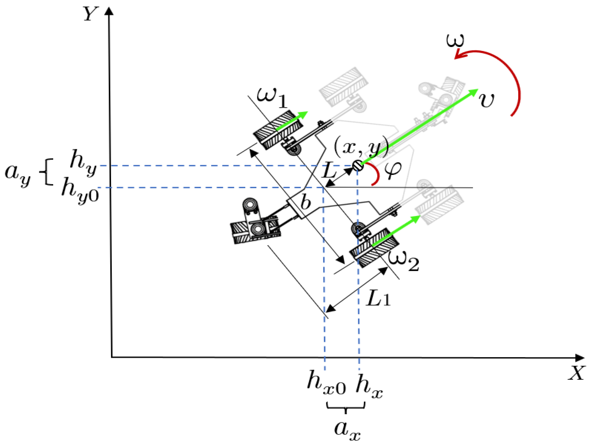
The proposed kinematic model is a simplification of the rover kinematics of this work, considering two-dimensional motion, as shown in Figure 2. With this model, the suspension joints, terrain inclinations and possible wheel slippage can be neglected to simplify the analysis; this enables the control of a complex robotic system by means of a simple control strategy. Consequently, since the kinematic loops in the suspension parallelograms can be ignored, which means that the translational and rotational velocities of the robot are not necessary in the control law, advantages in terms of analytical complexity are obtained over models such as those of Meghdari et al. [16], Li et al. [17] and Xu et al. [18], whose models present difficulties when implemented due to their inherent complexity. This is due in part to the difficulty of measuring variables, including wheel slip and the angles of suspension joints. Furthermore, these models also present difficulties when considering a position control law. Conversely, the proposed strategy can be applied to other rovers as long as their locomotion is close to differential guided locomotion and sensors with sufficient accuracy are available for the application. All of the aforementioned allow us to model and control only the rear half of the rover (the non-faded part of the robot in Figure 2), and due to the symmetry in its construction, this can be used to control the front half (the faded part of the robot in Figure 2). The modelling is performed considering the position and velocity of the control point located at the centre of gravity of the rover, denoted by the point ( x , y ) , which is initially assumed to be over the centre of the axis of the two side wheels.
The positions with respect to the actual point of control (centre of gravity) are given by
x = h x = h x 0 + a x = h x 0 + L cos ( φ ) y = h y = h y 0 + a y = h y 0 + L sin ( φ )
where h 0 x and h x are the positions of the centre wheel axle and the centre of gravity, respectively, on the x-axis, and h 0 y and h y on the y-axis. a x is the distance between h 0 x and h x , and a y is the distance between the positions h 0 y and h y .
Differentiating the positions from Equation (1), we obtain
x ˙ = h ˙ x 0 L φ ˙ sin ( φ ) y ˙ = h ˙ y 0 + L φ ˙ cos ( φ )
where h ˙ x 0 = υ cos ( φ ) and h ˙ y 0 = υ sin ( φ ) .
Then, substituting h ˙ x 0 and h ˙ y 0 into Equation (2) and adding the orienting velocity, we obtain the simplified kinematic model defined by
x ˙ y ˙ φ ˙ = cos ( φ ) L sin ( φ ) sin ( φ ) L cos ( φ ) 0 1 υ ω
The movement of the robot is given according to the angular velocities ( ω 1 , ω 2 ); for this reason, the model of Equation (3) must be expressed as a function of the rotational speeds of the side wheels, through the expressions of the differential guided locomotion of Baturone [20]. Let
υ ω = R 2 R 2 R b R b ω 1 ω 2
Then, substituting (4) into (3), we obtain the simplified model of the robot as follows:
x ˙ y ˙ φ ˙ = R cos φ 2 + L R sin φ b R cos φ 2 L R sin φ b R sin φ 2 L R cos φ b R sin φ 2 + L R cos φ b R b R b ω 1 ω 2
where x is the rover position on the x axis, y is the rover position on the y axis, φ is the rover’s orientation angle with respect to axis x, x ˙ is the rover speed on the x axis, y ˙ is the rover speed on the y axis, φ ˙ is the rover rotational speed or orientation, L is the perpendicular distance from the centre of the axis to the centre of gravity, L 1 is the perpendicular distance from the centre of the axle to the steering wheel, b is the rover road or distance between side wheels, and R is the wheel radius.
Thus, the model presented in Equation (5) represents, in a synthesised form, the main variables that relate the prototype kinematics, and the locomotion is then given by the angular velocities of the side wheels ω 1 and ω 2 .

4. Control Strategy

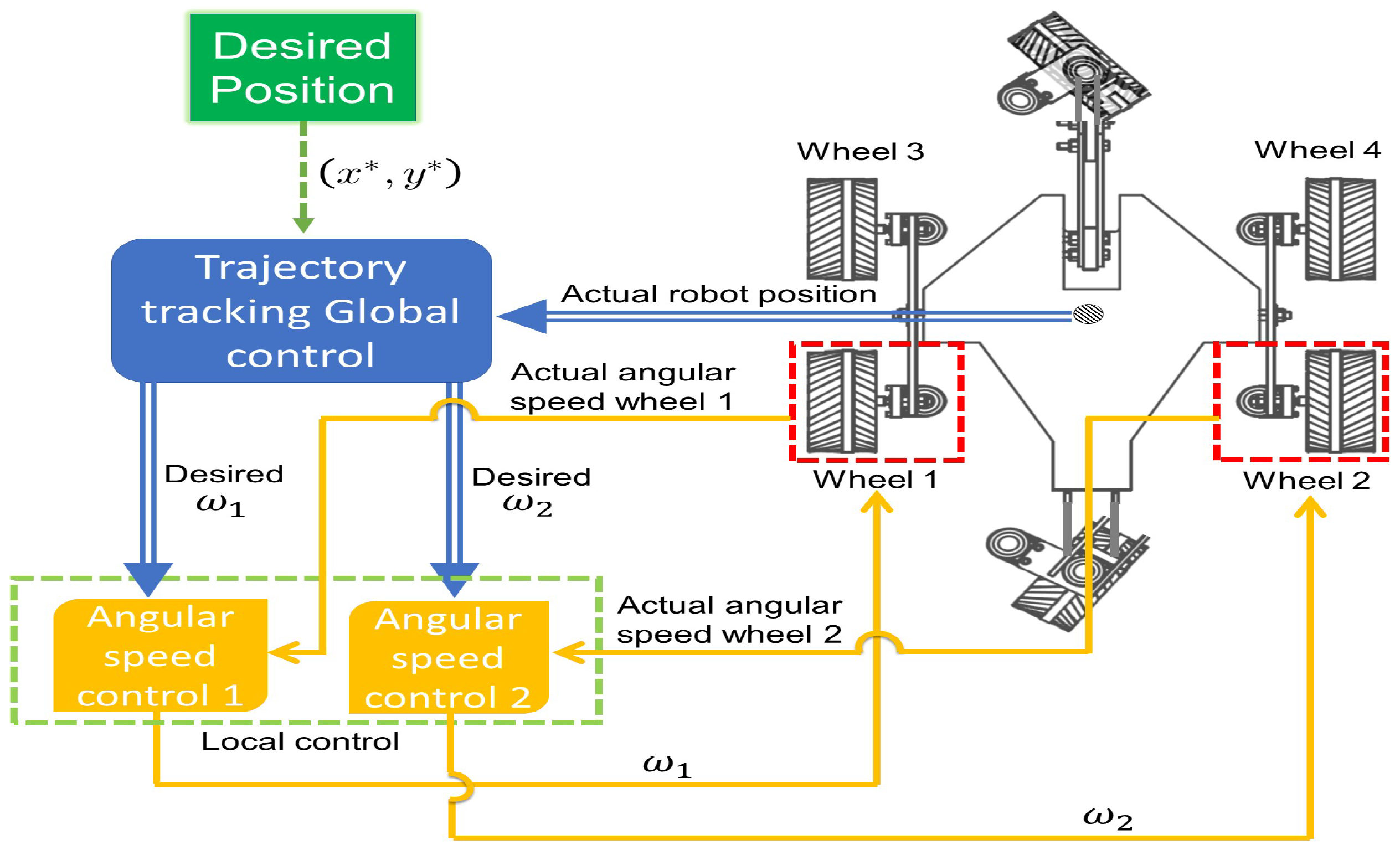
The locomotion system of the prototype is composed of two subsystems: the traction subsystem and the steering subsystem, each of which must be controlled independently. Due to these characteristics, the general control strategy is made up of two sub-strategies: “global control”, designed from the expression of the model (5), and “local control”, designed for each of the locomotion subsystems (six wheels and two steering mechanisms). The diagram in Figure 3 illustrates the basis of the control strategy, where it can be seen that the rover’s kinematics are a function of the angular velocities of wheels 1 and 2; from these, the other variables involved in the robot’s motion are generated, as in the case of the velocities of wheels 3 and 4, which must be equal to those of wheels 1 and 2, respectively. Likewise, the speeds of the front and rear wheels and the angle of the steering mechanisms are obtained from speeds 1 and 2. All of this make up the set of parameters necessary for trajectory tracking.

4.1. Trajectory Tracking Control—Global Control

In order to propose a control law of easy implementation and development that is related to the objectives of this work, a proportional type control is proposed; this is because in mobile robots based on differential configuration, this control proves to be sufficient and viable compared to other control strategies [21].
Proportional control can be defined in the time domain as u i = K p i e ( t ) , where e ( t ) is the difference between the desired output signal and the actual output signal. Let U = u 1 u 2 be the vector of proportional control actions with u 1 = υ and u 2 = ω , while understanding that υ is the displacement velocity vector in ( x , y ) coordinates and ω is the rover rotation velocity; the proportional controller is then equal to the right-hand side of Equation (3), and the position control law for the rover is given by
K p x ( x x ) K p y ( y y ) = cos ( φ ) L sin ( φ ) sin ( φ ) L cos ( φ ) υ ω
Solving for variables u 1 = υ and u 2 = ω , we have
u 1 u 2 = cos ( φ ) L sin ( φ ) sin ( φ ) L cos ( φ ) 1 K p x ( x x ) K p y ( y y )
where K p x and K p y are the controller constants for each coordinate, while ( x , y ) are the coordinates of the desired trajectory. To obtain the velocities ω 1 and ω 2 , which control the rover kinematics, from the control actions u 1 and u 2 , Equation (4) must be used again.

4.2. Locomotion Subsystem Control—Local Control

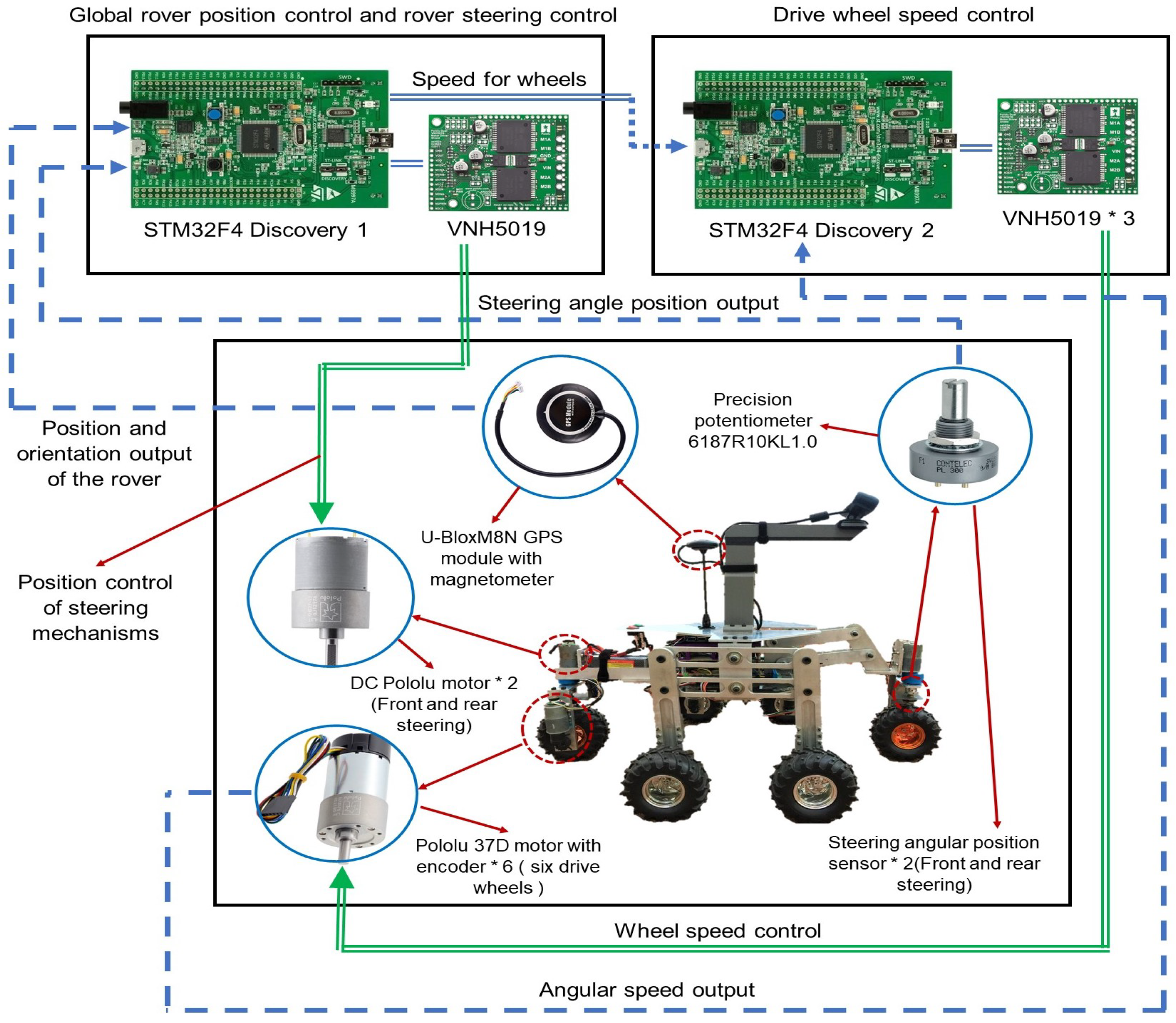
In order to control the angular positions of the two steering mechanisms, it is necessary to control the steering actuators themselves (Pololu 37D Metal Gear Motors with 131.25:1 Reduction); PID controllers are used for this purpose, since they have shown good results in mechanisms of this type [22]. The time domain PID control is as follows:
u p = k p s e s ( t ) + k i s 0 t e s ( τ ) d τ + k d s d e s ( t ) d t
where k p s , k i s and k d s are the proportional, integral and derivative constants for tuning the controller, and e s ( t ) is the position error. In the case of the angular velocity of the wheels, a PI-type control is considered sufficient, which is in agreement with the results of works such as [23]. The time domain PI control is defined as follows:
u v = k p ω e ω ( t ) + k i ω 0 t e ω ( τ ) d τ
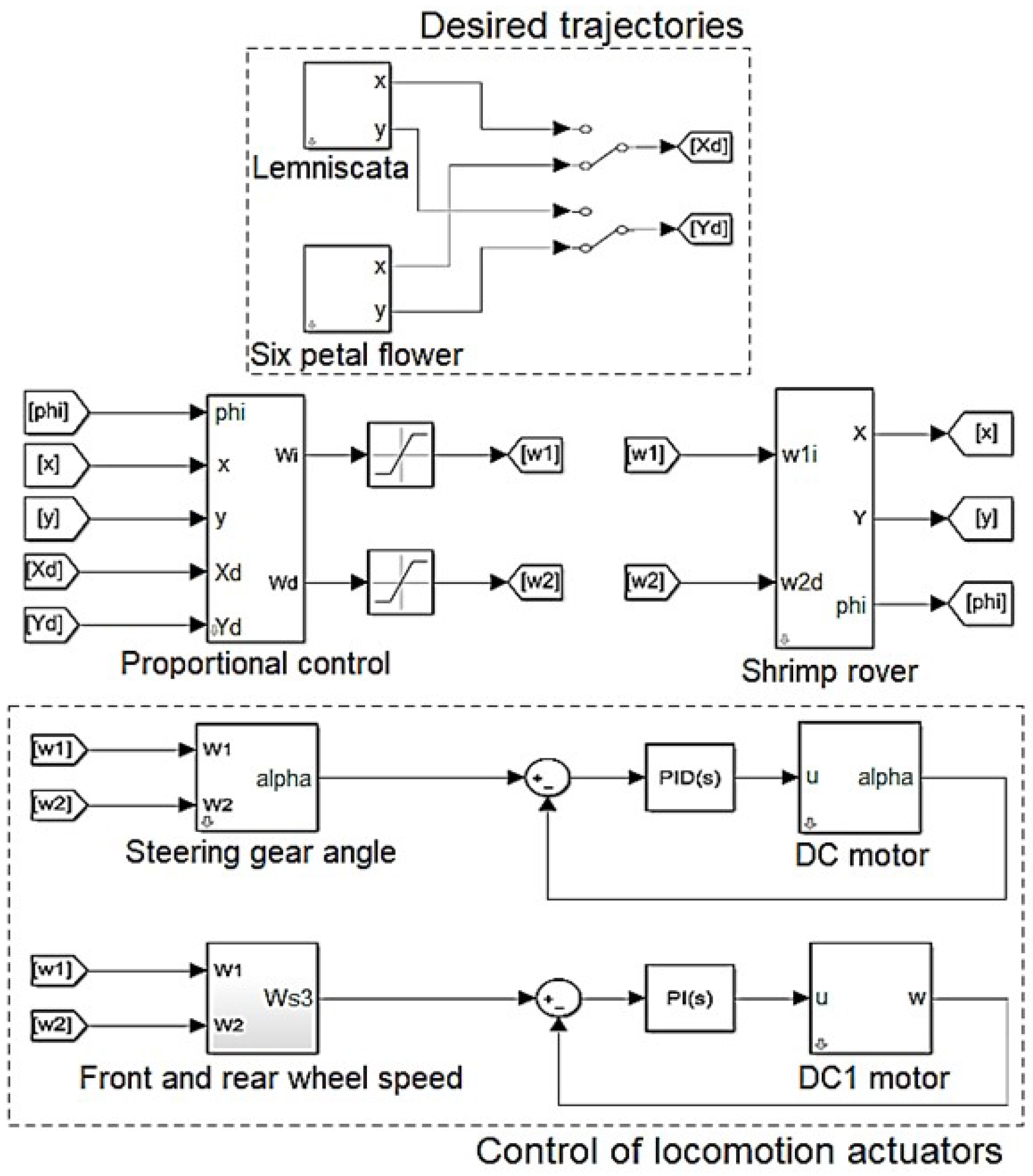
where k p ω and k i ω are the proportional and integral constants by which the control is tuned, and e ω ( t ) is the velocity error. The distribution of controllers involved in locomotion systems is shown in Figure 4.

4.3. Reference Signals for Motion Subsystem Controls

The global controller does not control the complete set of locomotion systems; consequently, the actuators of these systems must be driven according to the desired trajectory, so the steering mechanism must be positioned according to a signal that depends on the rover’s motion. Figure 4 shows the relationship between the reference signals and the different controllers.

4.3.1. Angle for Steering Mechanism

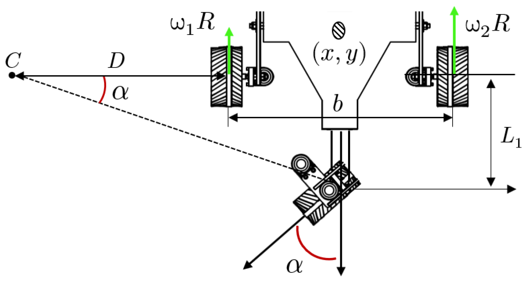
The angular position of the steering is given by the angle α (see Figure 5), which is the same for the front and rear mechanism but with an opposite direction of rotation. α must be set according to the difference in speed of the side wheels. As shown in Figure 5, when there is a difference between ω 1 R and ω 2 R , an instantaneous centre of rotation called C is generated, located at a distance D from the wheel closest to C.
Taking d s as the instantaneous displacement, decomposed into d s 1 for wheel 1 and d s 2 for wheel 2, we obtain [24]:
d s 1 = D d α = ω 1 R d t
d s 2 = ( D + b ) d α = ω 2 R d t
The expression for the length D is obtained by dividing (10) with (11):
D = ω 1 b ω 2 ω 1
In knowing the distance D, the reference angle α is given by Equation (13):
α = tan 1 L 1 D + b 2

4.3.2. Front and Rear Wheel Angular Velocity

The front ω F s and rear ω R s velocities must rotate according to the robot’s speed; these velocities must be adapted to the rover’s orientation behavior. If it moves only by making turns around the same point, the velocity of the front and rear wheels must be equal to those of the side wheels, regardless of the direction of rotation. In this case, the velocities will be equal but with opposite directions of rotation; thus ω F s and ω R s are obtained using Equation (14):
ω F s = ω R s = | ω 1 | + | ω 2 | 2
On the contrary, when the rover succeeds in orienting itself and starts the course toward the desired position, its linear velocity will be different from zero, and the velocities must be those necessary for each wheel to equal the linear velocity of the rover. In this case, the velocity is obtained with Equation (15):
ω F s = ω R s = ω 1 + ω 2 2

5. Numerical Simulation

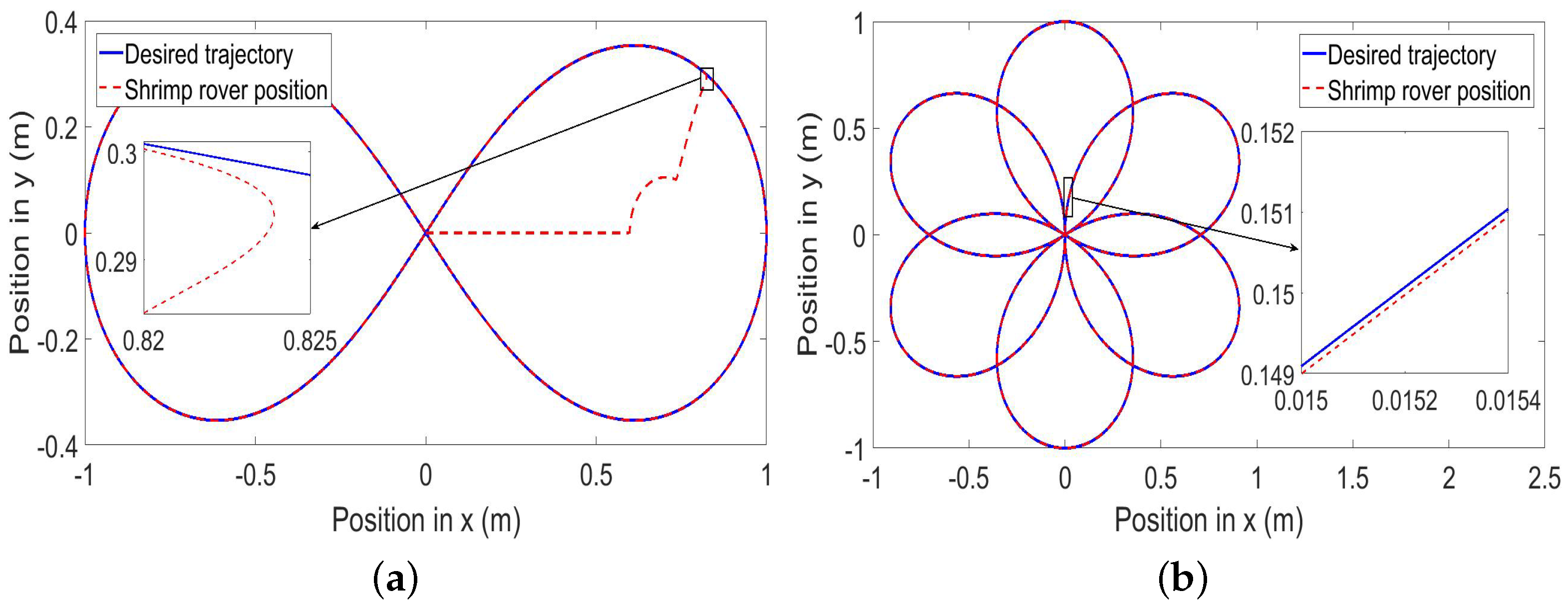
Using Matlab-Simulink, two desired trajectories were generated for the simulated rover path; one in the form of a six-petal flower with parametric equations that were taken as in [25] and the other in the form of a lemniscate. In this way, the response of the controllers to a variation in difficulty with respect to changes in direction was evaluated. The parametric equations for the lemniscate and flower trajectories are given by
x L = a L cos ( t ) 1 + sin 2 ( t ) y L = a L sin ( t ) cos ( t ) 1 + sin 2 ( t )
and
x F = a F sin ( 3 ω F t + η ) sin ( 2 ω F t + η ) y F = a F sin ( 3 ω F t + η ) cos ( 2 ω F t + η )
In Equation (16), x L , y L and a L are the path coordinates and the radius of curvature of the lemniscate, respectively; as in Equation (17), for the flower path, ω is also defined as the path frequency, and η , as the rotation parameter. In both trajectories, in order to test the performance of the strategy on paths shorter than those naturally followed by a rover type robot, the radius of curvature was set to 1 m. The other parameters are ω F = 0.5 and η = π . The general simulation scheme is shown in Figure 6.
The initial conditions were zero for all systems, while the local controller parameters were k p s = 882.235558229673 × 10 6 , k i s = 303.54182647177197 × 10 6 and k d s = 306.14244926964096 × 10 6 for the steering mechanism and k p ω = 305.131139982279 × 10 6 and k i ω = 144.272360647379 × 10 5 for the traction wheel.

5.1. Simulation Results of Trajectory Tracking

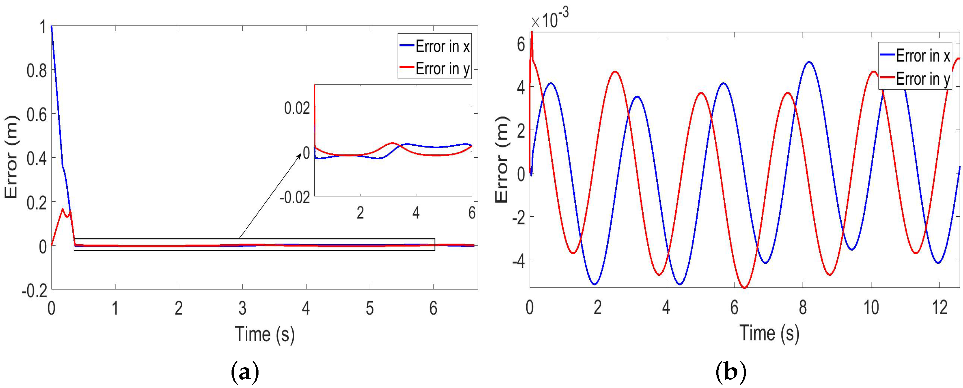
One way to assess the performance of a given control law involves an analysis of how closely a system responds to its desired behavior. In the particular case of the present work, the performances of all control strategies were obtained mainly by obtaining the error of the robot position, of the steering mechanisms and of the speed of the wheels while driving; the error is the difference between the signal of each system and its corresponding desired signal. Thus, Figure 7a,b show the path of the rover (red line) compared to the desired trajectory (blue line) using proportional control. Figure 8a,b show the error dynamics and indicate that with small deviations ranging from 0.02 to 0.02 for the lemniscate and from 5 × 10 3 to 5 × 10 3 for the flower trajectory, the robot follows the proposed paths, in addition to the trajectories reached before the first second of simulation. The low position error shows that proportional control based on the proposed kinematic model of the robot is suitable for different applications. Finally, the main data and results of this phase are shown in Table 2.

5.2. Control Results of Steering Mechanisms

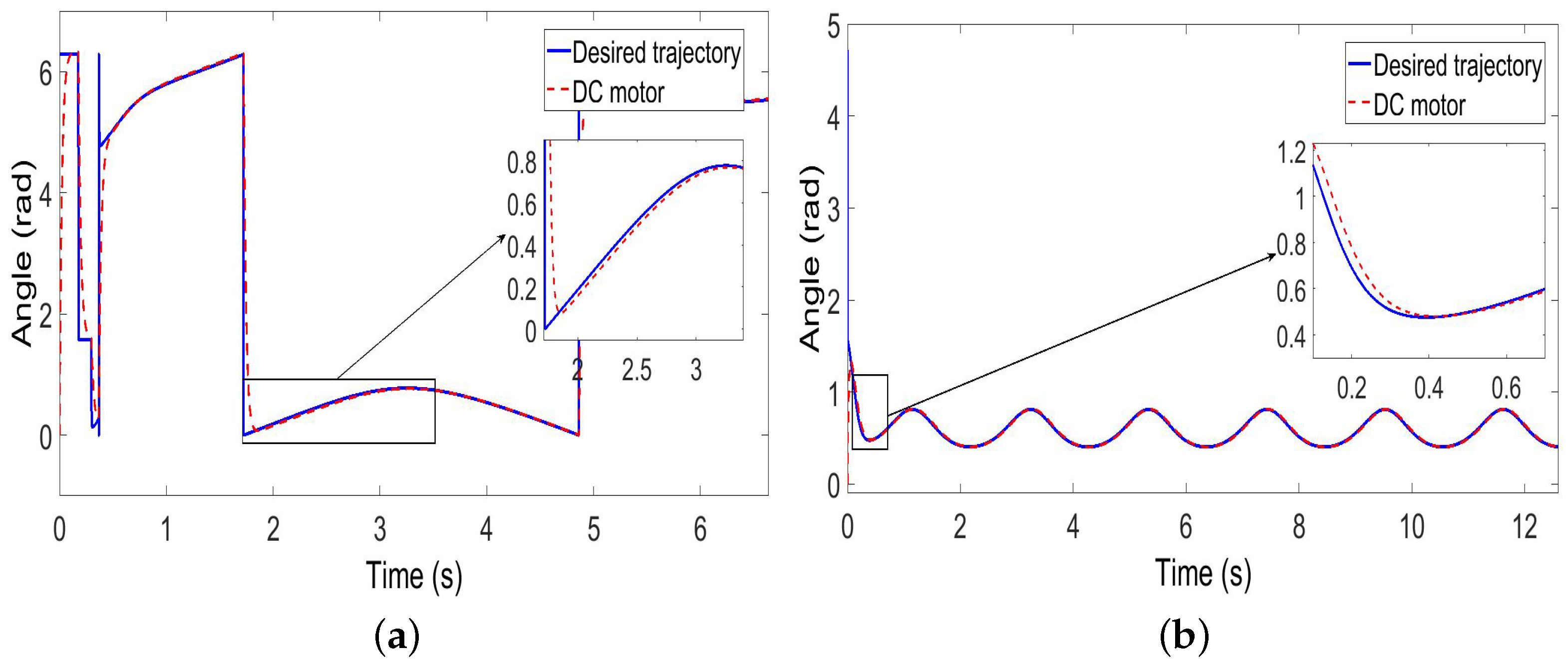
The behavior of the steering mechanism compared to the reference signal obtained with Equation (13) is shown in Figure 9a,b. The results show that the mechanism is positioned with a maximum error of 18.6506 × 10 3 rad in the flower trajectory and 29.4385 × 10 3 rad in the lemniscate trajectory between 1.9 and 4.8 s, excluding any error generated by sudden large angle changes.

5.3. Wheel Speed Control Results

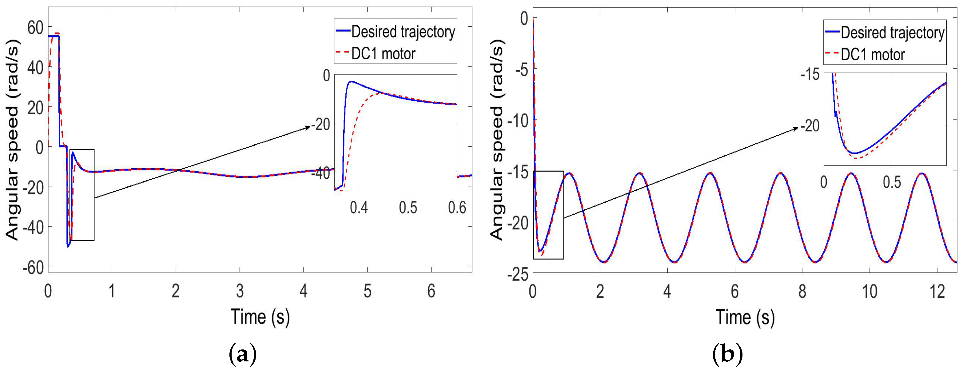
The results in Figure 10a,b correspond to the behavior of the traction motors under PI control, compared to the reference signal generated with Equations (14) and (15). The maximum errors after reaching the desired trajectory are 0.0623 rad/s for lemniscate and 0.2262 rad/s for the flower.

6. General Implementation and Experimental Testing

The implementation of the control algorithms is presented in this section. Figure 11 shows the prototype electronic instrumentation, which consists of two board based on an ARM Microcontroller used to calculate the control laws, GPS and magnetometer sensors to obtain the orientation and position and an actuator for each wheel of the robot. In this case, the entire strategy was programmed using Matlab-Simulink in conjunction with the Waijung blockset. The motion controllers were applied independently to each actuator. Here, a PID was implemented two times (two steering mechanisms), and a PI, six times (six drive wheels).

Experimental Results

With the diameter of the wheels being 124 mm, experimental tests were carried out on rough terrain with conditions that made it traversable for the prototype, i.e., obstacles smaller than twice the wheel diameter, 248 mm, and with transversal inclinations of less than 35° and longitudinal inclinations of less than 30°, according to the prototype design parameters presented in [19]. Travelling was conducted between two fixed geographic coordinates, where the longitude was considered as movement in x and latitude as movement in y. The test conditions and results are presented in Table 3, where some data were taken from the mobile application myTracks [26] along with the route captures (see Figure 12).
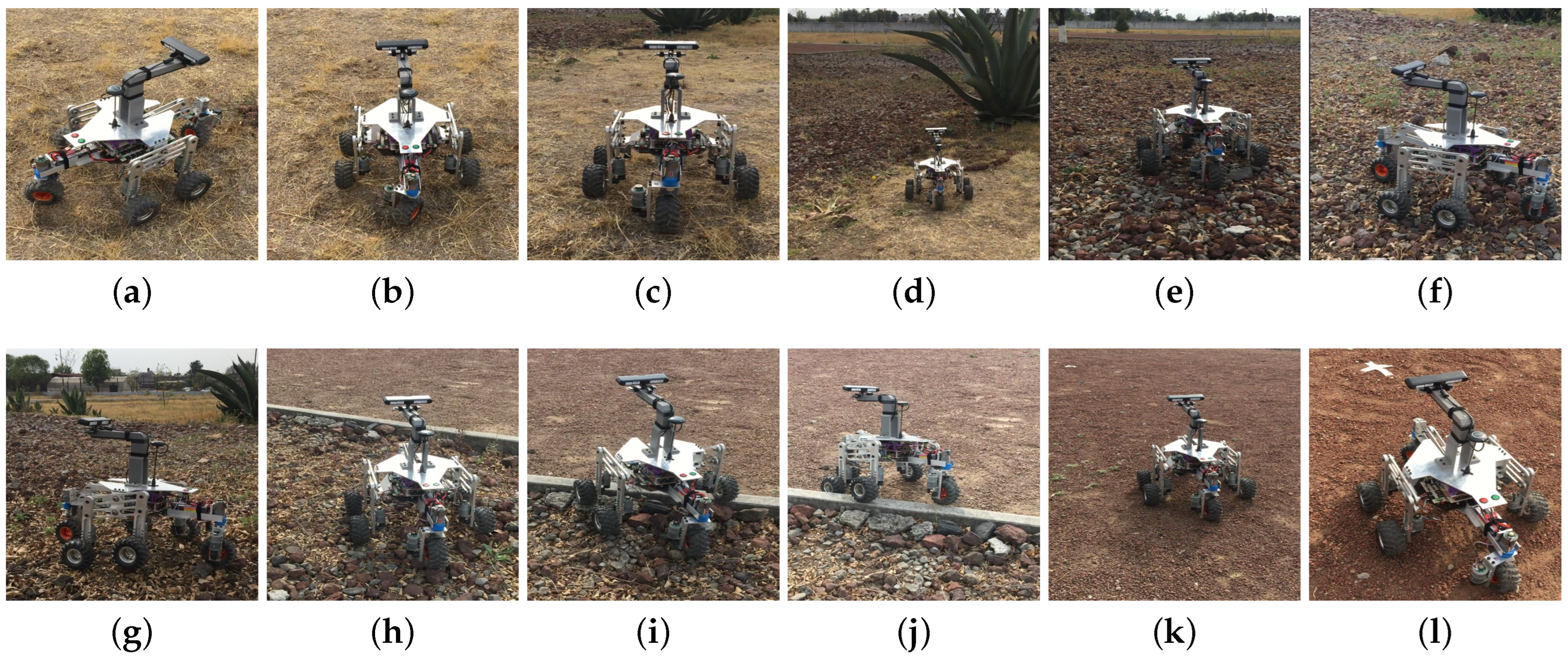
Figure 13 shows snapshots of the secondary test with the desired position ( L a t = 19.513667 ° ,   L o n g = 99.128389 ° ) and ( L a t = 19.513860 ° ,   L o n g = 99.1288299 ° ) as initial conditions. In Figure 13, the desired coordinate is marked with a white “X” on the ground. The position error of 1.9 m is within the 3 m success limits of the autonomous navigation test according to URC 2024 rules [27], so this result is sufficient according to the requirements of this competition. The position error may vary depending on the accuracy of the measurements, which implies better results under better measurement conditions, as in the case of the secondary test (Figure 13), where the rover was positioned only 30 cm from the target.

7. Conclusions

This work presents a control strategy for the trajectory tracking application of a passive suspension rover-type mobile robot. This strategy used an approximate kinematic model that allows a robot with complex suspension systems to be controlled using an easy control law. Also, we propose a control scheme in two control loops. The first closed loop is focused on the trajectory tracking of the kinematic model of the robot, and the second closed loop is designed for each of the locomotion subsystems.
This control schemes was implemented in a robotic system, which was a robot with a passive suspension that is capable of carrying out displacements over rough terrain and had electronic instrumentation that consisted of two boards based on an ARM Microcontroller used to calculate of control laws and condition the GPS and magnetometer sensors. Finally, the tests were performed through numerical simulations against different desired trajectories, and also using experimental tests using the embedded systems of the prototype, which showed an adequate performance despite the complexity of the rover and the terrain characteristics, with errors between 0.3 m and 1.9 m. These results are promising with regard to competitions such as the URC [27].
The following remarks can be stated:
  • The kinematic model allows us to treat the mobile system with a simplified approach that resembles a differential robot with a geometric centre at an eccentric point with respect to the axis centre. This configuration is very important to ensure holonomic restrictions in the system, reducing the control synthesis to a set of classic controls with a simple inverse gain compensation. Most approaches tend to use differential robot-based kinematic models with non-holonomic restrictions that are not addressed.
  • Even when the mechanical design and control ensure robustness against disturbances and certain slopes, actual applications demand a higher scale in both the size of the vehicle and the wheel radius to improve the capacity in rougher terrains.
  • The presented design obtains its position measurements using a GPS, and even when the system has an RGB-D camera, it is only used for obstacle detection, which may not be robust in practical tasks. In this sense, an area of opportunity consists of the inclusion of more sensors as well as the active use of an RGB-D camera to improve the robustness and accuracy of the position sensing by means of alternative approaches such as sensor fusion.

Author Contributions

Conceptualisation, J.D.D.-O., O.G.-F. and J.A.A.-A.; methodology, J.D.D.-O., J.A.A.-A. and A.L.-J.; software, J.D.D.-O.; validation, J.D.D.-O., J.A.A.-A., O.G.-F. and A.L.-J.; writing—original draft preparation, J.D.D.-O., J.A.A.-A. and O.G.-F.; writing—review and editing, O.G.-F. and A.L.-J.; visualisation, J.D.D.-O. and J.A.A.-A.; funding acquisition, O.G.-F., J.A.A.-A. and A.L.-J. All authors have read and agreed to the published version of the manuscript.

Funding

This research was funded by Secretaria de Investigación y Posgrado Instituto Politécnico Nacional under grants numbers 20240705, 20240693 and 20241802.

Institutional Review Board Statement

Not applicable.

Informed Consent Statement

Not applicable.

Data Availability Statement

Data are contained within the article.

Acknowledgments

Jheison Duvier Diaz-Ortega thanks the support from the CONAHCYT.

Conflicts of Interest

The authors declare no conflicts of interest.

References

  1. Sutoh, M. Traveling performance analysis of planetary rovers using a repeatable test system in vacuum. J. Terramech. 2021, 95, 15–24. [Google Scholar] [CrossRef]
  2. Lopez-Arreguin, A.J.R.; Montenegro, S. Machine learning in planetary rovers: A survey of learning versus classical estimation methods in terramechanics for in situ exploration. J. Terramech. 2021, 97, 1–17. [Google Scholar] [CrossRef]
  3. Bajracharya, M.; Maimone, M.W.; Helmick, D. Autonomy for Mars Rovers: Past, Present, and Future. Computer 2008, 41, 44–50. [Google Scholar] [CrossRef]
  4. Chen, C.; Shu, M.; Wang, Y.; Ding, L.; Gao, H.; Liu, H.; Zhou, S. Simultaneous control of trajectory tracking and coordinated allocation of rocker-bogie planetary rovers. Mech. Syst. Signal Process. 2021, 151, 107312. [Google Scholar] [CrossRef]
  5. Parsons IV, J.R.; Mazzoleni, A.P. Modeling and experimental investigation of the dynamics of a spherical Transforming Roving Rolling Explorer (TRREx) prototype. Acta Astronaut. 2021, 181, 92–111. [Google Scholar] [CrossRef]
  6. Sasiadek, J.; Green, D. Guidance and Control of Autonomous Planetary Rover. IFAC Proc. Vol. 1997, 30, 241–246. [Google Scholar] [CrossRef]
  7. Caracciolo, L.; De Luca, A.; Iannitti, S. Trajectory tracking control of a four-wheel differentially driven mobile robot. In Proceedings of the 1999 IEEE International Conference on Robotics and Automation (Cat. No. 99CH36288C), Detroit, MI, USA, 10–15 May 1999; Volume 4, pp. 2632–2638. [Google Scholar]
  8. Yang, J.M.; Kim, J.H. Sliding mode control for trajectory tracking of nonholonomic wheeled mobile robots. IEEE Trans. Robot. Autom. 1999, 15, 578–587. [Google Scholar] [CrossRef]
  9. Sasiadek, J.; Lu, Y. Path tracking of an autonomous LHD articulated vehicle. IFAC Proc. Vol. 2005, 38, 55–60. [Google Scholar] [CrossRef]
  10. Grand, C.; Benamar, F.; Plumet, F. Motion kinematics analysis of wheeled–legged rover over 3D surface with posture adaptation. Mech. Mach. Theory 2010, 45, 477–495. [Google Scholar] [CrossRef]
  11. Arabi, A.A.; Sakib, H.U.; Sarkar, P.; Proma, T.P.; Anowar, J.; Amin, M.A. Autonomous Rover Navigation Using GPS Based Path Planning. In Proceedings of the 2017 Asia Modelling Symposium (AMS), Kota Kinabalu, Malaysia, 4–6 December 2017; pp. 89–94. [Google Scholar] [CrossRef]
  12. Polash, M.M.H.; Tumpa, S.N.; Saumik, S.S.; Samia, M.B.R.; Rafid, M.F.; Elahi, S.S.B.; Moumi, P.K.; Dipta, S.R.; Inan, T.T.; Oishwee, S.J.; et al. Explorer-0100: An autonomous next generation Mars rover. In Proceedings of the 2017 20th International Conference of Computer and Information Technology (ICCIT), Dhaka, Bangladesh, 22–24 December 2017; pp. 1–7. [Google Scholar] [CrossRef]
  13. Zhang, W.; Gai, J.; Zhang, Z.; Tang, L.; Liao, Q.; Ding, Y. Double-DQN based path smoothing and tracking control method for robotic vehicle navigation. Comput. Electron. Agric. 2019, 166, 104985. [Google Scholar] [CrossRef]
  14. Qi, L.; Zhang, T.; Xu, K.; Pan, H.; Zhang, Z.; Yuan, Y. A novel terrain adaptive omni-directional unmanned ground vehicle for underground space emergency: Design, modeling and tests. Sustain. Cities Soc. 2021, 65, 102621. [Google Scholar] [CrossRef]
  15. Khan, R.; Malik, F.M.; Raza, A.; Mazhar, N. Comprehensive study of skid-steer wheeled mobile robots: Development and challenges. Ind. Robot. Int. J. Robot. Res. Appl. 2020, 48, 142–156. [Google Scholar] [CrossRef]
  16. Meghdari, A.; Mahboobi, S.; Gaskarimahalle, A.L. Dynamics modeling of “cedra” rescue robot on uneven terrains. In Proceedings of the ASME International Mechanical Engineering Congress and Exposition, Anaheim, CA, USA, 13–19 November 2004; Volume 47063, pp. 991–1001. [Google Scholar]
  17. Li, S.; Liu, J.; Sun, M.; Wen, W.; Bi, S. Optimal design for a self-adaptive mobile robot based on virtual center of motion. In Proceedings of the 2009 IEEE International Conference on Robotics and Biomimetics (ROBIO), Guilin, China, 19–23 December 2009; pp. 414–419. [Google Scholar]
  18. Xu, M.; Yang, R.; Cheng, Y.; Xu, H. Kinematics modeling and step climbing study of an all-terrain wheeled mobile robot on uneven terrains. In Proceedings of the 2011 International Conference on Electronic & Mechanical Engineering and Information Technology, Harbin, China, 12–14 August 2011; Volume 5, pp. 2725–2728. [Google Scholar]
  19. Aguirre-Anaya, J.A. Diseño y Construcción de un Móvil Tipo Rover de Arquitectura Abierta. Master’s Thesis, Instituto Politecnico Nacional—Unidad Profesional Interdisciplinaria en Ingeniería y Tecnologías Avanzadas, Ciudad de México, Mexico, 2016. Available online: https://cloud.upiita.ipn.mx/s/bRRCGpjFXawpzrN (accessed on 13 March 2024).
  20. Baturone, A.O. Robótica: Manipuladores y Robots Móviles; Marcombo, 2005. [Google Scholar]
  21. Sugisaka, M.; Hazry, D. Development of a proportional control method for a mobile robot. Appl. Math. Comput. 2007, 186, 74–82. [Google Scholar] [CrossRef]
  22. Haytham, A.; Elhalwagy, Y.; Wassal, A.; Darwish, N. Modeling and simulation of four-wheel steering unmanned ground vehicles using a PID controller. In Proceedings of the 2014 International Conference on Engineering and Technology (ICET), Cairo, Egypt, 19–20 April 2014; pp. 1–8. [Google Scholar]
  23. Kanojiya, R.G.; Meshram, P. Optimal tuning of PI controller for speed control of DC motor drive using particle swarm optimization. In Proceedings of the 2012 International Conference on Advances in Power Conversion and Energy Technologies (APCET), Mylavaram, India, 2–4 August 2012; pp. 1–6. [Google Scholar]
  24. Sira-Ramirez, H.; Agrawal, S.K. Differentially Flat Systems, 1st ed.; CRC Press: Boca Raton, FL, USA, 2004. [Google Scholar]
  25. Luviano-Juárez, A.; Cortés-Romero, J.; Sira-Ramírez, H. Trajectory tracking control of a mobile robot through a flatness-based exact feedforward linearization scheme. J. Dyn. Syst. Meas. Control. 2015, 137, 051001. [Google Scholar] [CrossRef]
  26. Hanson, B.A.; Seeger, C.J. Apps for Collecting GPS Tacks: MyTracks-The GPS-Logger. 2015. Available online: https://store.extension.iastate.edu/product/Apps-for-Collecting-GPS-Tracks-myTracks-The-GPS-Logger (accessed on 14 November 2023).
  27. Mars Society. University Rover Challenge. 2006. Available online: https://urc.marssociety.org/home/requirements-guidelines (accessed on 14 November 2023).
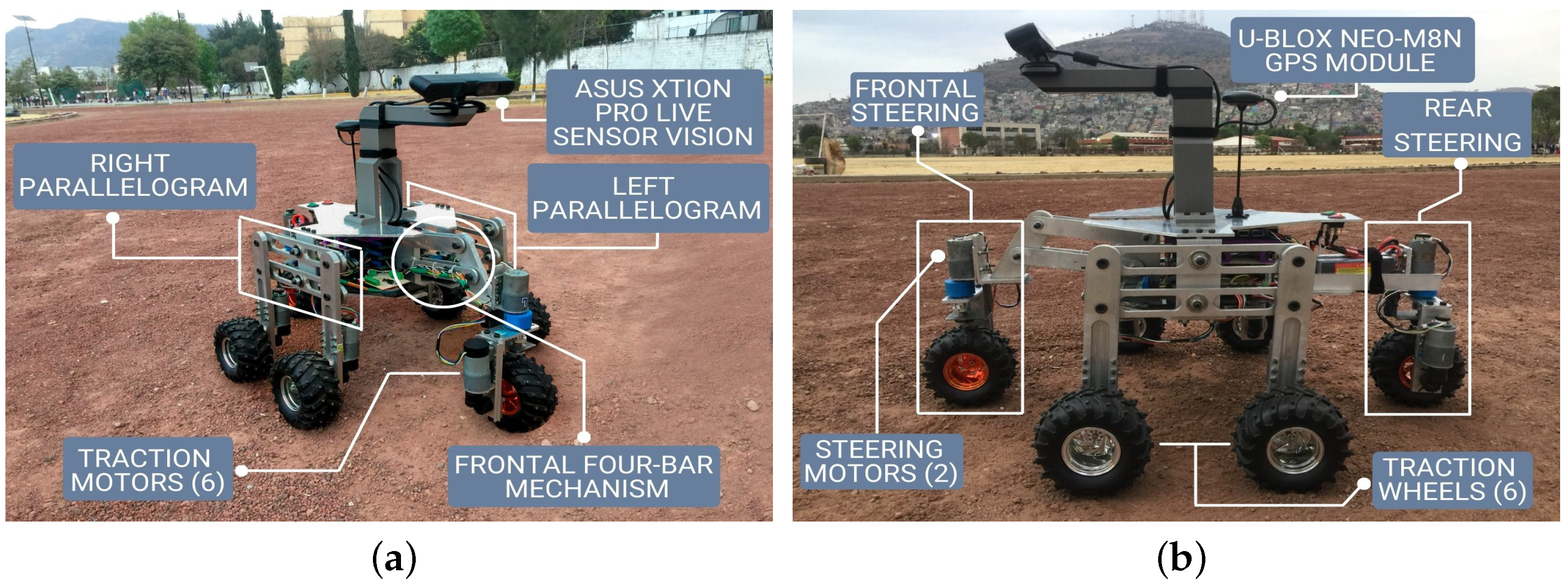
Figure 1. Actuators, sensors and rover subsystems. (a) Suspension; (b) traction and steering.
Machines 12 00322 g001
Figure 2. Model diagram.
Machines 12 00322 g002
Figure 3. General control strategy diagram.
Machines 12 00322 g003
Figure 4. General control block diagram.
Machines 12 00322 g004
Figure 5. Steering angle.
Machines 12 00322 g005
Figure 6. General simulation diagram.
Machines 12 00322 g006
Figure 7. Rover behavior in trajectory tracking. (a) Lemniscata; (b) six-petal flower.
Machines 12 00322 g007
Figure 8. Position error in trajectory tracking. (a) Lemniscate; (b) six-petal flower.
Machines 12 00322 g008
Figure 9. Steering behavior in trajectory tracking. (a) Lemniscate; (b) six-petal flower.
Machines 12 00322 g009
Figure 10. Angular velocity behavior of wheels in trajectory tracking. (a) Lemniscate; (b) six-petal flower.
Machines 12 00322 g010
Figure 11. General implementation distribution.
Machines 12 00322 g011
Figure 12. Route of the main test. (a) Satellite view; (b) enlarged satellite view.
Machines 12 00322 g012
Figure 13. Test positioning sequence.
Machines 12 00322 g013
Table 1. Used prototype main features [19].
FeaturesDescription
Prototype dimensions50.5 cm × 75 cm × 60 cm
Model dimensionsL = 0.105 m, L 1 = 0.315 m, R = 0.062 m, b = 0.445 m
Weight9.5 kg
Number of wheels6
Suspension systemParallelogram
Traction systemEach wheel is actuated
Steering systemWorks independently on front and rear wheels
Obstacles to overcomeObstacles with a height of twice its wheel diameter
Processing cards2 STM32F4 Discovery microcontrollers
Localisation moduleGPS U-BloxM8N
ActuatorsGeared motors with encoder pololu 37D-131.25:1
Motor controllers4 drivers pololu VNH5019 Dual
Table 2. Summary of simulation results.
TrajectoryVariableQuantity
LemniscateMaximum position error in x0.0032 mm
Maximum position error in y0.0036 mm
Initial conditions ( x , y ) (0, 0) m
Wheels’ maximum angular velocity55 rad/s
Time to reach the desired trajectory<1 s
Controller’s gains K p x = 277, K p y = 277
Six-petal flowerMaximum position error in x0.0051 mm
Maximum position error in y0.0053 mm
Initial conditions ( x , y ) (0, 0) m
Wheels’ maximum angular velocity55 rad/s
Time to reach the desired trajectory<1 s
Controller’s gains K p x = 283, K p y = 283
Table 3. Test conditions and results and simplified model parameters.
ParameterUnitsValue
Initial positionLat = 19.512416, Long = −99.127674
Initial orientationrad5.7596
Desired coordinatelat = 19.513616, long = −99.128438
Max. wheel speedr/min40
Controller constants K p x = 278; K P y = 278
Travel timemin11.267
Distance coveredm174
Mean travel speedm/s0.2574
Final positionLat = 19.513605, Long = −99.128425
Positioning errorm1.9
Lm0.105
L 1 m0.315
Rm0.062
bm0.445
Disclaimer/Publisher’s Note: The statements, opinions and data contained in all publications are solely those of the individual author(s) and contributor(s) and not of MDPI and/or the editor(s). MDPI and/or the editor(s) disclaim responsibility for any injury to people or property resulting from any ideas, methods, instructions or products referred to in the content.