Article

Simulation and Validation of an 8 × 8 Scaled Electric Combat Vehicle

Department of Automotive and Mechatronics Engineering, Ontario Tech University, 2000 Simcoe ST N, Oshawa, ON L1G 0C1, Canada
*
Author to whom correspondence should be addressed.
Machines 2024, 12(2), 146; https://doi.org/10.3390/machines12020146
Submission received: 25 December 2023 / Revised: 31 January 2024 / Accepted: 18 February 2024 / Published: 19 February 2024
(This article belongs to the Special Issue Intelligent Control and Active Safety Techniques for Road Vehicles)

Abstract

:
In this research, an 8 × 8 scaled electric combat vehicle (SECV) is built. The scaled vehicle is evaluated in both experimental and simulated methods to analyze its performance. The scaled vehicle is developed to apply the Ackermann condition by implementing the individual steering and individual wheel speed control system at low speed. Individual eight-wheel rotational velocity control and individual eight-wheel steering angle control in real time are developed and installed on the remotely controlled scaled vehicle to meet a perfect Ackermann condition. Three different steering scenarios are developed and applied: a traditional steering scenario (first and second axle steering), fixed third axle steering scenario (first, second, and fourth axle steering), and all-wheel steering scenario. Stationary evaluation, turn radius evaluation, and double lane change evaluation are conducted to verify the application of the Ackermann condition. The differences between the experimental results and the simulated data are within an acceptable range. An important demonstration of this research is the novel validation of physical and simulated data in the application of the Ackermann condition for eight-wheel steering and velocity control for the three steering scenarios.

1. Introduction

1.1. Literature Review

Over the last few years, steering and velocity control of vehicle stability systems have been improved incredibly. The research areas of Ackermann’s condition and controllers implemented on steering strategy were reviewed at the beginning of this research. For instance, two applied controllers, Linear Time-Invariant (LTI) and Linear Parameter-Varying (LPV), were developed by Selmanaj et al. (2013) [1]. The benefits of rear-wheel steering are demonstrated in four-wheeled vehicles utilizing the global chassis control strategy by showing two different controllers. The simulated data of the rear-wheel steering show advanced dynamic behaviors of vehicles at high speed and in harsh driving conditions [1].
Unlike Selmanaj’s two applied controllers [1], the performance of the 8 × 8 heavy combat vehicle is represented with all ranges of velocity to prove the advantage of the controller steering strategy by D’Urso [2] in 2016. In the same year, D’Urso [2] developed and implemented multiple controllers to improve the maneuverability of the 8 × 8 heavy combat vehicle at a large range of speeds. For instance, the low-speed test is conducted on the combat vehicle equipped with A ZSS (zero side slip) controller that works on the last two axles’ steering [2]. Moreover, simulated evaluations (TruckSim simulation) including NATO double lane change (DLC) and constant turn radius test are conducted to analyze the application of the steering control strategy on the 8 × 8 heavy combat vehicle [2].
Implementing the complete Ackermann equation shows a huge number of advantages, especially for heavy multi-axle vehicles in terms of vehicle maneuverability, and this is demonstrated by Zhang et al. (2022) [3]. For example, an incredibly reduced tire skid is observed by implementing the complete Ackermann equation. Moreover, the enhanced dynamic stability of the heavy-duty multi-axle vehicle is another advantage of the complete Ackermann strategy [3]. To meet the requirement of the Ackermann equation on the heavy-duty vehicles, a two degrees of freedom (DOF) electro-hydraulic servo steering system (TDEHSSS) is developed and implemented by Zhang et al. (2022) [3]. The results of the implementation of the complete Ackermann strategy on the heavy-duty multi-axle vehicle are represented by Zhang et al. (2022) in terms of steering characteristics and tire wear [3].
Ma et al. [4] applied the Ackermann steering strategy to minimize the lateral skid effect by designing a bigger inner wheel angle than the outer wheel angle. For instance, the intersection between the perpendicular bisectors of the front wheels and the rear axle determines the Instantaneous Center of Rotation (ICR) [4]. The experimental evaluations were conducted to validate their simulated data [4]. For instance, they represent that the Ackermann visual-inertial odometry (ACK-MSCKF) equipped with the Ackermann steering strategy improves trajectory estimation from 59.85% to 67.70% in the 160 m length of the experimental test [4]. Vehicle dynamic components such as gravity center position and inertial parameters were obtained by Yu et al. in 2017 [5] with CarSim/Simulink to represent the evaluation of Ackermann’s steering strategy. It is shown by Ye et al. (2017) [5] that tire force data are not required to calculate steering angles by applying Ackermann’s steering geometry. For example, the effect of tire slip at low-speed test is ignored theoretically by the definition of Ackermann’s steering geometry.
Another strategy was developed for vehicle control systems in which experimental evaluation was conducted by Girbacia et al. (2018) [6]. For instance, the Ackermann steering method is applied to an autonomous vehicle to minimize lateral skid when the autonomous vehicle keeps track of a predefined path following [6]. Furthermore, Girbacia et al. (2018) [6] obtained a data sample of the velocity variation during simulated experiments to implement an Ackermann steering strategy.
In 2020, Ataei et al. [7] established and integrated a multi-objective control system for electric vehicles to obtain a few main goals in terms of control strategy. The integrated control system designed by Aboelfadl et al. [8] represents improved stability of the vehicle dynamic. The main concerns of vehicle stability are slip control of traction and braking, stability of lateral motion, controllability, and prevention of rollover when designing the control system of the electric vehicle. Model predictive control (MPC) was developed to maintain the vehicle’s dynamic stability by distributing the correct amount of torque to four independent wheels of the electric vehicle. In 2020, Zhang et al. [9] also showed another active front wheel steering control system with a direct yaw moment control strategy, and it was proved by representing the simulation result of the performance of the integrated nonlinear robust adaptive controller. In 2022, Changoski et al. [10] suggested two different steering controllers, including an active front steering controller and an active rear steering controller. ADAMS/Car software (Version 2022a) was used to perform a simulated evaluation on a B-segment vehicle to obtain the goal of this research. Matlab/Simulink software was also used to compare the simulation results as an evaluation tool.
A controller implemented on an automated vehicle regarding path-following strategies was introduced by Zhou et al. in 2021 [11]. The proposed controller showed the result of minimized energy consumption and the highest level of stability compared to the traditional model (H∞). Moreover, experimental tests were conducted on a scaled vehicle to validate the simulation results of the proposed controller [11]. The simulated tests of a scaled electric vehicle (1:10 ratio) were conducted by Samada et al. in 2023 [12]. Path-following strategies for racing cars were introduced based on historical data obtained from many experimental tests. For instance, the error between the target path and the actual path was maintained within the acceptable range, and input efforts were minimized by the robust controllers including ZKF, MPC, and LQZ [12]. A controller equipped with a disturbance observer was developed to minimize the effect of disturbance by Guevara et al. in 2023 [13]. For example, the proposed controller was installed on a general n-trailer to enhance the performance of trajectory tracking in real-life driving conditions. Both experimental and simulated tests were conducted for the validation of the improvement, including a 57% reduction in error compared to the traditional model [13].
In 2022, Tan et al. [14] performed the path planning of high-level model and low-level vehicle dynamic control methods for an autonomous parking and navigation strategy on a scaled 8 × 8 electric combat vehicle. However, there were limitations regarding the vehicle’s dynamic control [14]. For that reason, in 2023, Kim et al. [15] continued Tan’s research, using a scaled 8 × 8 electric combat vehicle, and enhanced the scaled vehicle’s dynamic control system by implementing a high-level vehicle control strategy. For instance, this high-level vehicle control strategy refers to the complete Ackermann equation responsible for the individual steering angle and the individual wheel velocity. The study implemented a remote-control system to maneuver the scaled vehicle by a human driver in a traditional steering scenario. The study was the first to validate experiment and simulation evaluation regarding the scaled 8 × 8 electric combat vehicle with an independent steering and wheel speed control system. Building on this research, this paper demonstrates and adds two other steering scenarios: the fixed third axle steering scenario and all-wheel steering scenario.

1.2. Contributions

This research contains the first demonstration of the validity of the complete Ackermann condition among three novel steering scenarios for a scaled electric combat vehicle undertaking a low-speed maneuver. For instance, accurate maneuvering at a low speed is often necessary for military combat vehicles during military operations. Therefore, implementing the complete Ackermann strategy on a full-size heavy combat vehicle is vital for a successful military operation at low speed by minimizing lateral skid and enhancing maneuverability. The primary objective of this study is to substantiate the advantages associated with the implementation of the fixed third axle scenario and the all-wheel steering scenario in comparison to the traditional steering scenario. This will be achieved by presenting the results of the turn radius, which were obtained through two distinct methods. These turn radius results will then be employed to assess the lateral skid in three different scenarios, as the lateral skid significantly influences the controllability of the scaled vehicle. The all-wheel steering scenario demonstrates superior turn radius results, showcasing minimal lateral skid and thereby indicating enhanced controllability. Another aim of this study is to validate the scaled vehicle by comparing experimental and simulation results. This validation process allows the experimental data of the scaled vehicle to be extrapolated for estimating the full-size vehicle dynamics. Furthermore, the comprehensive Ackermann strategy employed in this study holds potential benefits for the driving performance of multi-axle heavy trucks, especially in scenarios where these trucks are required to operate at low speeds.

1.3. Challenges

The developed mathematical model relationships do not require any control implementation since they implement Ackermann’s condition to control the scaled vehicle during a low-speed test. In future research, a rear active steering controller will be developed and implemented to maneuver the scaled vehicle during a high-speed test. This rear active steering controller will overcome the limitations of the application of Ackermann condition, as the Ackermann condition is suitable only for the low-speed range. Tire force parameters will be estimated to compose mathematical equations of the rear active steering control system in the next study.

2. Hardware and Mathematical Model

In this section, the scaled vehicle’s mechanical design and sensors are introduced to explain how the Ackerman condition is implemented in the steering and speed control system. Moreover, vehicle mathematical models of three steering scenarios are represented by figures and equations to prove the application of the Ackermann condition.

2.1. Mechanical Design and Sensors

In this section, the installed electronic sensor, electronic equipment, and mechanical components are explained. A laptop equipped with an Intel Core-i5 processor and 16 GB RAM is installed on the first layer of the scaled vehicle. The experimentally obtained 1st axle inner wheel angle, yaw rate, longitudinal velocity, lateral acceleration, and trajectory are sent to the laptop for storing the result data. For instance, the 1st axle inner wheel angle is measured by a linear actuator sensor, and the trajectory is measured by an indoor GPS. The yaw rate and lateral acceleration are measured by an inertial measurement unit (IMU). Longitudinal velocity is measured by GPS. The IMU (RSX UM7 Orientation Sensor) [16] has three sub-sensors including a magnetometer, accelerometer, and gyroscope. The GPS (Locosys mc-1513) [17] measuring longitudinal velocity generates a position error within 3 m. The GPS can measure up to 515 m/s. The input values, including the steering angle and longitudinal velocity manipulated by a human driver, are created by a remote controller (Logitech F710 USB controller) [18]. The command signals (input values) are transmitted to the main Arduino by a USB host shield.
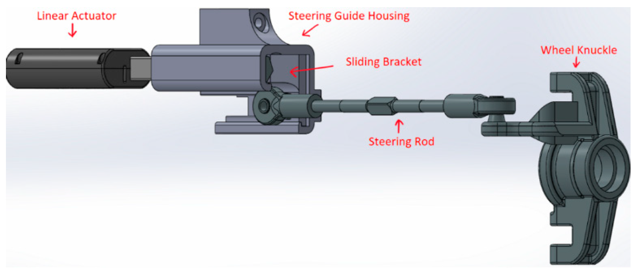
The scaled vehicle is equipped with three Arduino Mega 2560s to operate the individual steering and individual wheel speed control system. The main board, one of the three Arduinos, receives the single speed and the single steering input values from the remote controller. The main board performs mathematical calculations to maintain the control system regarding eight-wheel steering angles and eight-wheel velocities in real time. The two Arduinos are used as sub-boards to maintain and control eight-wheel steering angles (linear actuators) in real time based on the output values of the main board. For instance, these two sub-boards are connected to the main board to receive the main board’s output values. A proportional integral derivative (PID) closed-loop controller is implemented on the two sub-boards to control the linear actuators that have mechanical linkage with the steering rods. Figure 1 illustrates the diagram of the closed-loop controller applied to the linear actuator in the steering system. The stroke position of the linear actuator decides the steering angle of each wheel based on the simplified Equation (1). In this equation, l, rt, and θt represent the change in the stroke position, the radius of the tire, and the steering wheel angle. Figure 2 describes the steering assembly including the linear actuator, steering rod, and steering housing.
l = rtθt
First, 12 V power is transmitted to eight linear actuators from a battery (nickel–metal hydride battery 12 V 2800 mAh). The scaled vehicle has four motor controllers (Roboteq SDC2130) on the first layer, and two DC motors are controlled by each motor controller. The first axle’s motor controller is allocated as a main motor controller receiving the desired input speed from the main board. The main motor controller sends the desired input speed to the remaining three motor controllers. A PID controller, closed-loop velocity control, is implemented in four motor controllers to operate the eight-wheel performance. The motor controllers use eight encoders, AMT10 Rotary Encoders [19], connected to eight wheels to obtain feedback for the PID closed-loop velocity control system. Each Lipo battery, Gens ace 6200 mAh 14.8 V 45 C [20], provides power to each motor controller controlling two wheels on the same axle.
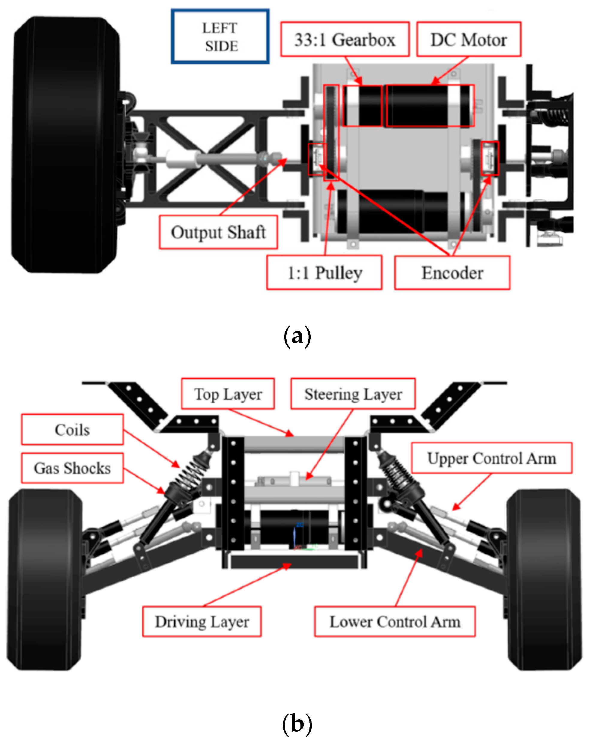
The scaled vehicle’s driving system and suspension system are shown in Figure 3a,b. For instance, each motor is connected to each wheel through the output shaft to transmit driving force and generate brake through the PID closed-loop control system. The upper control arm, lower control arm, coils, and gas shocks are composed to support the scaled vehicle’s body. Each suspension system connected to each wheel supports the unsprung weight of the scaled vehicle individually. Finally, indoor GPS [21] is used to measure the trajectory of the scaled vehicle during the double lane change (DLC) evaluation.

2.2. Vehicle Mathematical Model

In this section, the steering and wheel speed control methods for the scaled vehicle are explained. A real-time turning center is represented as P, and a longitudinal velocity is shown as V at point C in Figure 4, Figure 5 and Figure 6. Point C indicates the center of gravity in Figure 7; however, point C of Figure 5 and Figure 6 is not the center of gravity. Point C is located on the center line of the scaled vehicle and is the point that has the shortest distance from point P during cornering performance in Figure 5, Figure 6 and Figure 7. In this study, experimental and simulation tests are conducted at 5 km/h (equivalent to 30 km/h of the full-size vehicle) and low speed, since the mathematical models implemented in the scaled vehicle are kinematic models which do not include dynamic effects of wheel skid, body pitch, and body roll. The Ackermann condition equation is developed and applied to the scaled vehicle to analyze vehicle dynamic performance during continuous remote control test in terms of individual steering and individual wheel speed control systems. The unit and definition of parameters mentioned below are represented in Appendix A.
R = L 1 t a n δ i 1 + B 2
δ ij = tan 1 ( L j R B / 2 ) ;   δ oj = tan 1 ( L j R + B / 2 )
R ij = L j s i n δ i j ;   R oj = L j s i n δ o j
θ ˙ = V R
V ij = θ ˙ R i j ;   V oj = θ ˙ R o j
V i 3 = θ ˙ ( R B 2 ) ;   V o 3 = θ ˙ ( R + B 2 )
V i 4 = θ ˙ ( R B 2 ) ;   V o 4 = θ ˙ ( R + B 2 )
In Figure 4, Figure 5 and Figure 6, θ, δij, and δoj indicate yaw, each axle’s inner wheel angle, and each axle’s outer wheel angle. In addition, B and L indicate the track width and the wheelbase. Each axle’s inner and outer wheel velocity are described as Vij and Voj.
Equation (3) explains how each wheel angle is determined according to the turning radius (R) that has the shortest distance between the horizontal line of the vehicle and point P (turning center).
The steering angle input from the remote controller is sent to the first axle’s inner wheel ( δ i 1 ) through Arduino, since the first axle inner wheel always has the largest wheel angle based on the Ackermann condition equation. For instance, when the remote controller decides the first axle’s inner wheel angle ( δ i 1 ), Arduino calculates the turning radius (R) of the scaled vehicle in real time based on Equation (2). The real-time rest wheel angles including first axle outer, second axle inner, and second axle outer angles are calculated based on the instantaneous turning radius (R) by Equation (3). In this case, j is equal to 1 or 2.
In this study, Equations (4)–(8) are developed and implemented on the scaled vehicle to control each wheel speed individually. Therefore, the scaled vehicle can meet Ackerman’s condition to minimize tire skid at low-speed tests. For example, the first and second axle wheel’s turning radius is determined through Equation (4) to calculate each wheel’s individual speed. In this case, j is equal to 1 or 2. Moreover, the remote controller determines the longitudinal velocity (V) by using Arduino. With the allocated longitudinal velocity and the calculated turning radius from the first axle inner wheel angle, the angular velocity can be calculated by Equation (5). The scaled vehicle has the same angular velocity at any point, since the scaled vehicle is considered a rigid body. Equations (6)–(8) show how eight wheels achieve different individual velocities in real time to apply the mathematical model. In this case, j is equal to 1 or 2. However, the third and fourth axle’s wheels do not completely meet Ackermann’s condition, since the four wheels always have fixed steering wheel angles in the traditional steering scenario. For instance, Equations (7) and (8) show that each inner and outer estimated turning radius is applied on the third and fourth axle to calculate the third and fourth axle’s wheel velocities. To overcome this limitation, fixed 3rd axle and all-wheel steering scenarios are developed and introduced. Fixed 3rd axle and all-wheel steering modes will be explained in more detail in the next paragraph.
R = L 1 t a n δ i 1 + B 2
δ ij = tan 1 ( L j R B / 2 ) ; δ oj = tan 1 (   L j R + B / 2   )
R ij = L j s i n δ i j ; R oj = L j s i n δ o j
θ ˙ = V R
V i 3 = θ ˙ ( R B 2 ) ; V o 3 = θ ˙ ( R + B 2 )
V ij = θ ˙ R i j ; V oj = θ ˙ R o j
Equations (9) and (10) explain how each wheel angle is determined in Figure 5 according to the turning radius (R) that has the shortest distance between the center line of the vehicle and point P (turning center). In this case, j is equal to 1, 2, and 4.
The steering angle input from the remote controller is sent to the first axle’s inner wheel ( δ i 1 ) through Arduino, since the first axle inner wheel always shows the largest wheel angle based on the Ackermann condition equation. For instance, when the remote controller decides the first axle’s inner wheel angle ( δ i 1 ), Arduino calculates the turning radius (R) of the scaled vehicle in real time based on Equation (9) in Figure 5. The real-time rest wheel angles including the first, second, and fourth axles are calculated based on the instantaneous turning radius (R) by Equation (10). In this case, j is equal to 1, 2, and 4.
In this study, Equations (11)–(14) are developed and implemented on the scaled vehicle to control each wheel speed individually in Figure 5. Therefore, the scaled vehicle can meet Ackerman’s condition to minimize tire slip at low-speed tests. For example, each wheel’s turning radius is determined through Equation (11) to calculate each wheel’s individual speed in Figure 5 in terms of the first, second, and fourth axles. In this case, j is equal to 1, 2, and 4. The third axle’s turning radius is defined as R. Moreover, the remote controller determines the longitudinal velocity (V) by using Arduino. With the allocated longitudinal velocity and the calculated turning radius from the first axle’s inner wheel angle, the angular velocity can be calculated by Equation (12) in Figure 5. The scaled vehicle has the same angular velocity at any point, since the scaled vehicle is considered a rigid body. Unlikely the traditional steering scenario’s mathematical model, Equations (13) and (14) (fixed-third axle steering scenario) show how eight wheels achieve different individual velocities in real time to apply the condition of Ackermann’s theory in Figure 5. In this case, j is equal to 1, 2, and 4.
R = L 1 t a n δ i 1 + B 2
δ ij = tan 1 ( L j R B / 2 ) ; δ oj = tan 1 ( L j R + B / 2 )
R ij = L j s i n δ i j ; R oj = L j s i n δ o j
θ ˙ = V R
V ij = θ ˙ R i j ; V oj = θ   ˙ R o j
Equations (15) and (16) explain how each wheel angle is determined in Figure 6 according to the turning radius (R) that has the shortest distance between the horizontal line of the vehicle and point P (turning center). In this case, j is equal from 1 to 4.
The steering angle input from the remote controller is sent to the first axle’s inner wheel ( δ i 1 ) through Arduino, since the first axle’s inner wheel is always supposed to have the largest wheel angle based on the Ackermann condition equation. For instance, when the remote controller decides the first axle’s inner wheel angle ( δ i 1 ), Arduino calculates the turning radius (R) of the scaled vehicle in real time based on Equation (15) in Figure 6. The real-time rest wheel angles ( δ o 1 , δ i 2 , δ o 2 , δ i 3 , δ o 3 , δ i 4 , a n d   δ o 4 ) are calculated based on the instantaneous turning radius (R) by Equation (16). J is equal from 1 to 4 in Equation (16).
In this study, Equations (17)–(19) are developed and implemented on the scaled vehicle to control each wheel speed individually in Figure 6. In this case, j is equal from 1 to 4. Therefore, the scaled vehicle can meet Ackerman’s condition to minimize lateral skid in a low-speed test. For example, each wheel’s turning radius is determined through Equation (18) to calculate each wheel’s individual speed in Figure 6, and j is equal from 1 to 4. Moreover, the remote controller determines the longitudinal velocity (V) by using Arduino. With the allocated longitudinal velocity and the calculated turning radius from the first axle’s inner wheel angle, the angular velocity can be calculated by Equation (18) in Figure 6. The scaled vehicle has the same angular velocity at any point, as the scaled vehicle is considered a rigid body. Unlikely the traditional steering scenario’s mathematical model, Equation (19) (all-wheel steering scenario) shows how eight wheels achieve different individual velocity in real time to apply the condition of Ackermann’s theory in Figure 6. In this case, j is equal from 1 to 4.

3. Results

In this section, the validation and substantiation of the Ackerman condition discussed in the previous section through the examination of stationary, turn radius, and double lane change evaluations were elucidated. Specifically, a comparative analysis of three distinct steering methods utilizing both simulated and experimental data for a comprehensive assessment is presented.

3.1. Stationary Evaluation

The scaled vehicle’s length, width, and height are 1.13 m, 0.5 m, and 0.45 m. This dimension design is developed to implement a 1:6 scale ratio in terms of size between the scaled vehicle and the full-size vehicle. A 1:6 ratio is selected by considering the highest speed of the full-size combat vehicle. For example, with the maximum velocity of the full-size combat vehicle (100 km/h), the scaled vehicle needs the theoretical maximum speed of 16.67 km/h to apply the ratio of a 1:6 condition. However, the scaled vehicle’s current maximum speed is 6.7 km/h driving in a straight line due to the limitation of battery capacity. For that reason, stationary evaluation is conducted at the longitudinal velocity of 5 km/h (equivalent to 30 km/h of the full-size vehicle) to achieve the speed of eight wheels. The 1:6 ratio is based on the dimension ratio between scaled vehicle and full-size vehicle. The longitudinal velocity, trajectory, and lateral acceleration are calculated using the ratio of 1:6 between the scaled and full-sized vehicle based on Equations (20) and (22). Moreover, in this case, the scaled vehicle and the full-sized vehicle produce the same values regarding the time duration of the tests and the yaw rate. Therefore, an estimated lateral acceleration of the full-size vehicle (six times larger than the scaled vehicle) can be obtained by conducting an experimental test of the scaled vehicle. This is the most important benefit to using the scaled vehicle. However, there are some limitations regarding using the scaled vehicle when evaluating vehicle dynamic behaviors. For instance, vehicle sideslip does not have a linear relationship between the scaled vehicle and the full-size vehicle, as the steering angle of the scaled vehicle has a nonlinear relationship with the full-size vehicle. Developing a look-up table regarding the vehicle sideslip ratio between the scaled vehicle and the full-size vehicle with variables including velocity and turning radius will be a method to overcome this limitation. Our future research will use this look-up table to maximize the benefits of using the scaled vehicle. The mathematical model of a scaled vehicle among three different steering scenarios is demonstrated by confirming the results of the stationary evaluation. For instance, the speeds of eight wheels are measured by a tachometer every 2 degrees when the first axle inner wheel’s angle increases from 0 to 24 degrees. To overcome the noise caused by the tachometer, ten trials of measuring eight-wheel velocities were conducted every 2 degrees. In addition to that, the average of the ten trials is used in the experimental results of stationary evaluation. The process of stationary evaluation is shown in Figure 7 where the scaled vehicle is located on the jack for the test. The control input value of steering and velocity are determined by updating the Arduino code every 2 degrees to send accurate command signals. The results of stationary evaluation represent a left cornering and describe how eight-wheel velocities are changed with the increase in steering input value at 5 km/h (longitudinal velocity).

Wheel Rotational Speed and Radius of Vehicle Path

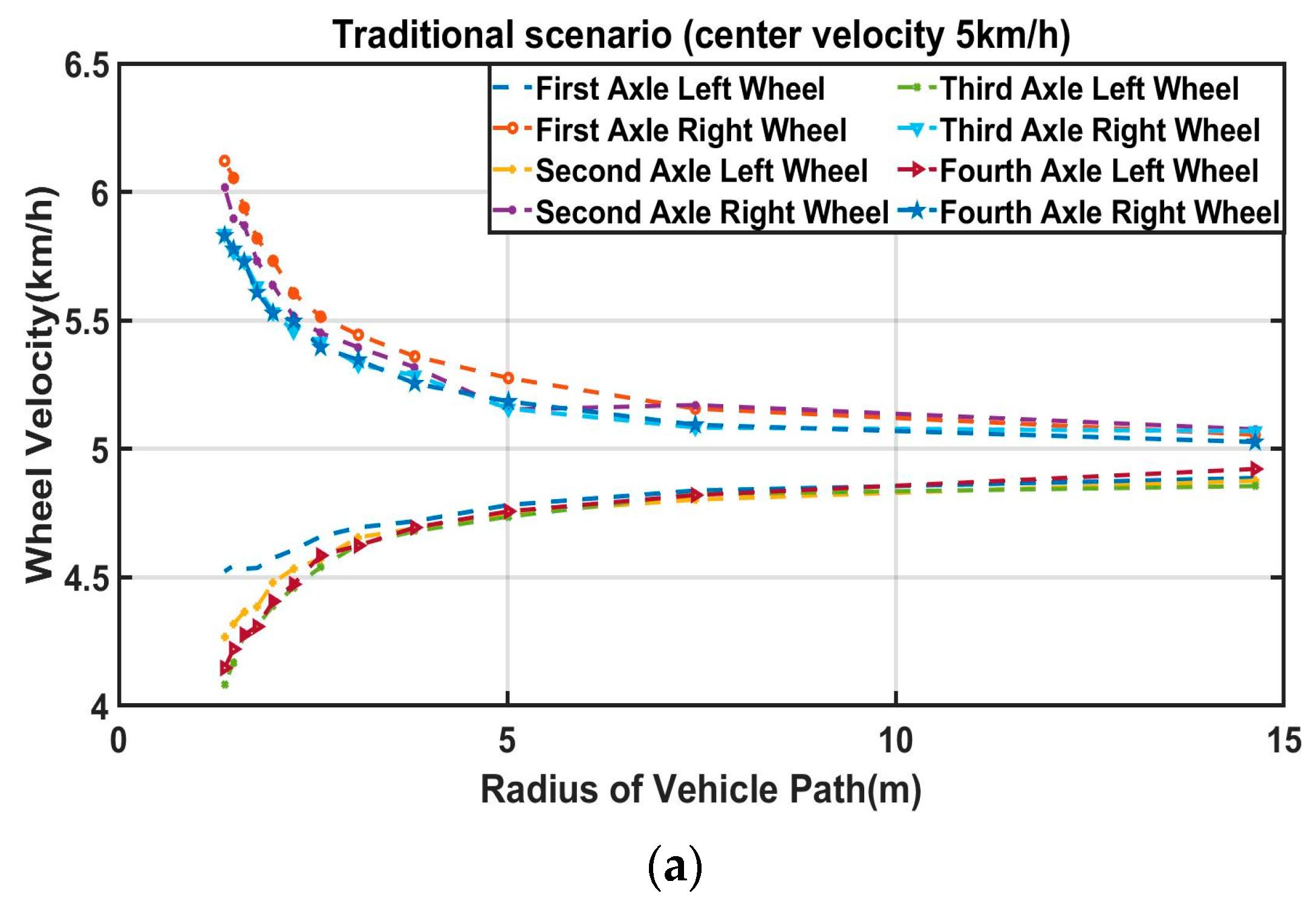
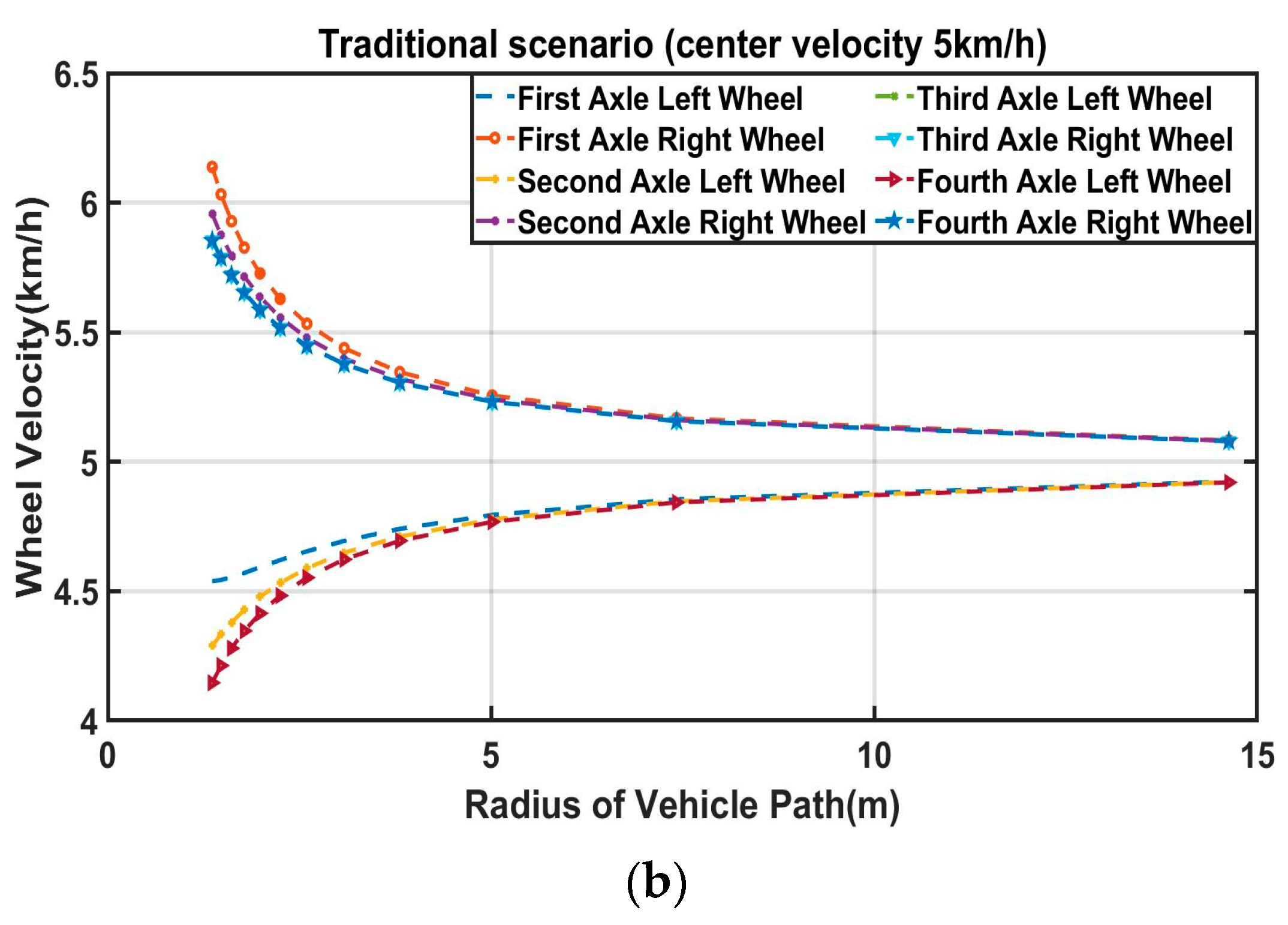
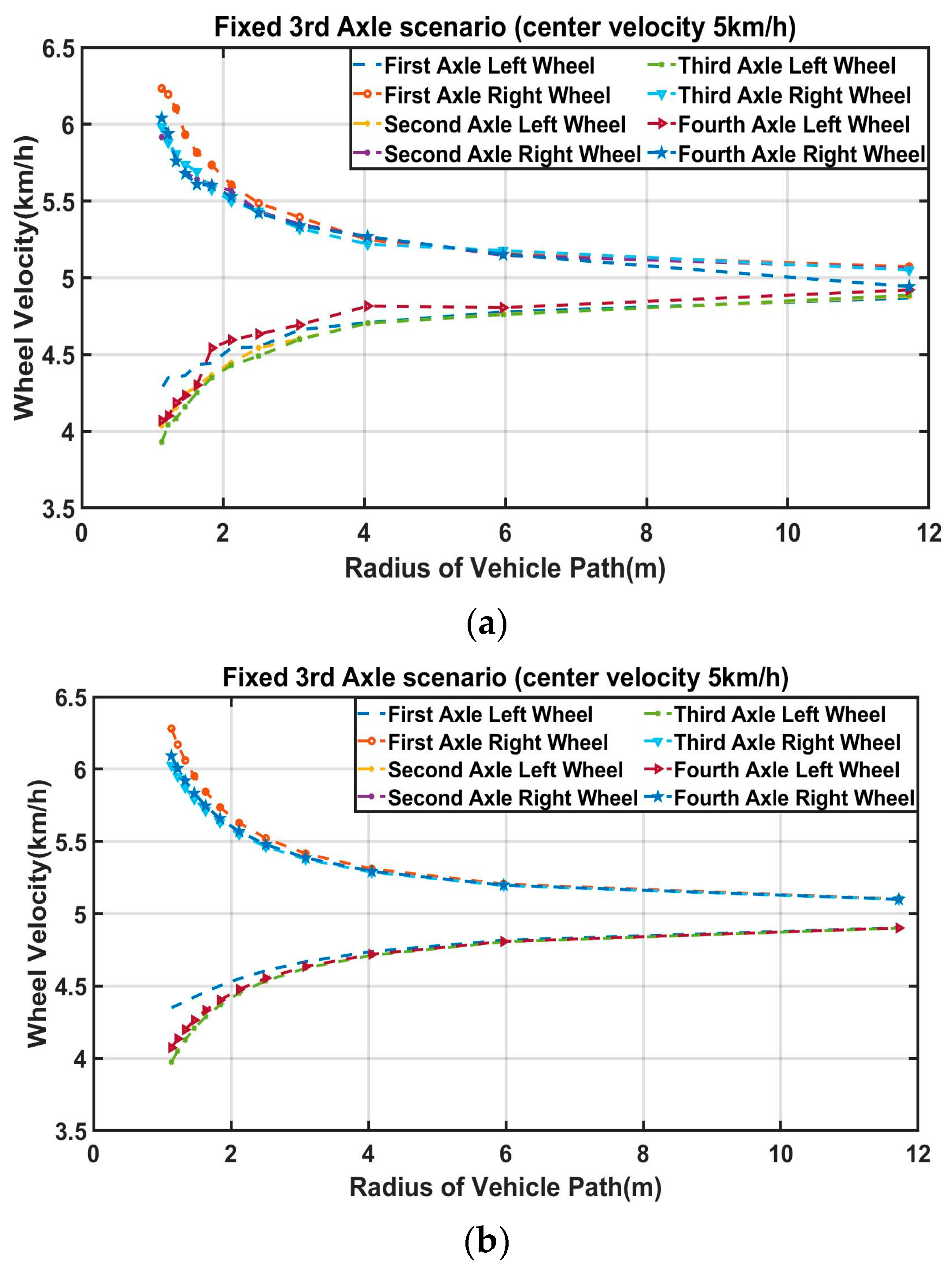
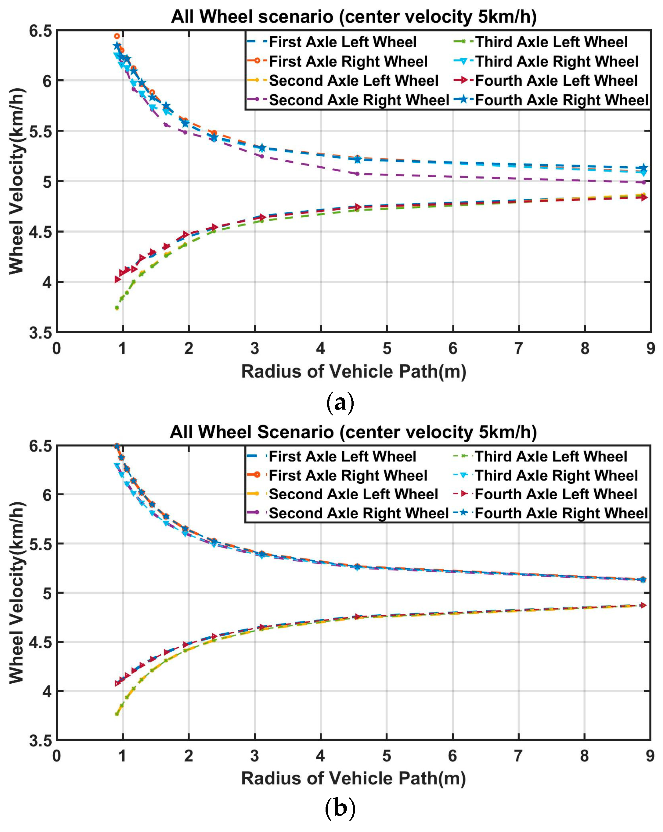
The eight wheels’ rotational velocities with the radius of the vehicle path are shown among three different steering scenarios in Figure 8, Figure 9 and Figure 10. The simulation data of the stationary test are obtained by MATLAB based on the mathematical equations previously mentioned above in Equations (2)–(19). The experimental results of stationary evaluation are achieved by the tachometer, and the procedure is explained in the previous paragraph. In Figure 8, Figure 9 and Figure 10, simulated and experimental data are presented to confirm that the desired eight-wheels velocities based on the vehicle mathematical model have the same values as the experimentally measured data. For instance, both experimental and simulated results generally show similar shapes.
In Figure 8, Figure 9 and Figure 10, the all-wheel steering scenario shows the largest difference between maximum speed and minimum speed among eight wheels at the maximum steering input (24 degrees) compared to the other two steering scenarios. Therefore, the maximum range of each wheel’s velocity should be higher in an all-wheel steering scenario to implement the vehicle mathematical model properly. Referring to the vehicle mathematical model explained previously, Figure 8, Figure 9 and Figure 10 show that the first axle right wheel always has the highest speed, since the vehicle is turning left during the stationary evaluation. However, in the all-wheel steering scenario, as shown in Figure 10, both the first axle’s right wheel and the fourth axle’s right wheel show the maximum speed with the same amount, as the all-wheel steering scenario has a symmetric design against the center gravity. After completing a stationary evaluation, it is seen that introducing a higher-performance encoder would be advantageous for minimizing the error between simulation and experimental data in future studies.

3.2. Turn Radius Evaluation

Turn radius evaluation is used to obtain the minimum turning radius on dry asphalt using the three different steering scenarios when the scaled vehicle is driven with maximum steering input at the highest speed. The three different steering scenarios indicate traditional, fixed-third axle, and all-wheel steering. The scaled vehicle is tested through turn radius evaluation in both simulated and experimental methods to achieve the 1st axle inner wheel angle, yaw rate, longitudinal velocity, lateral acceleration, trajectory, turning radius, and vehicle sideslip. The experimental data of turn radius evaluation are compared to the simulation data for validation purposes. With this comparison, the simulation data of TruckSim are proven, as it has very small errors compared to the experimental data. In the turn radius test, the scaled vehicle is driven with only a left turn, and a left turn is shown as a positive sign in all data.

Turn Radius Evaluation at Maximum Speed and Maximum Steering Angle

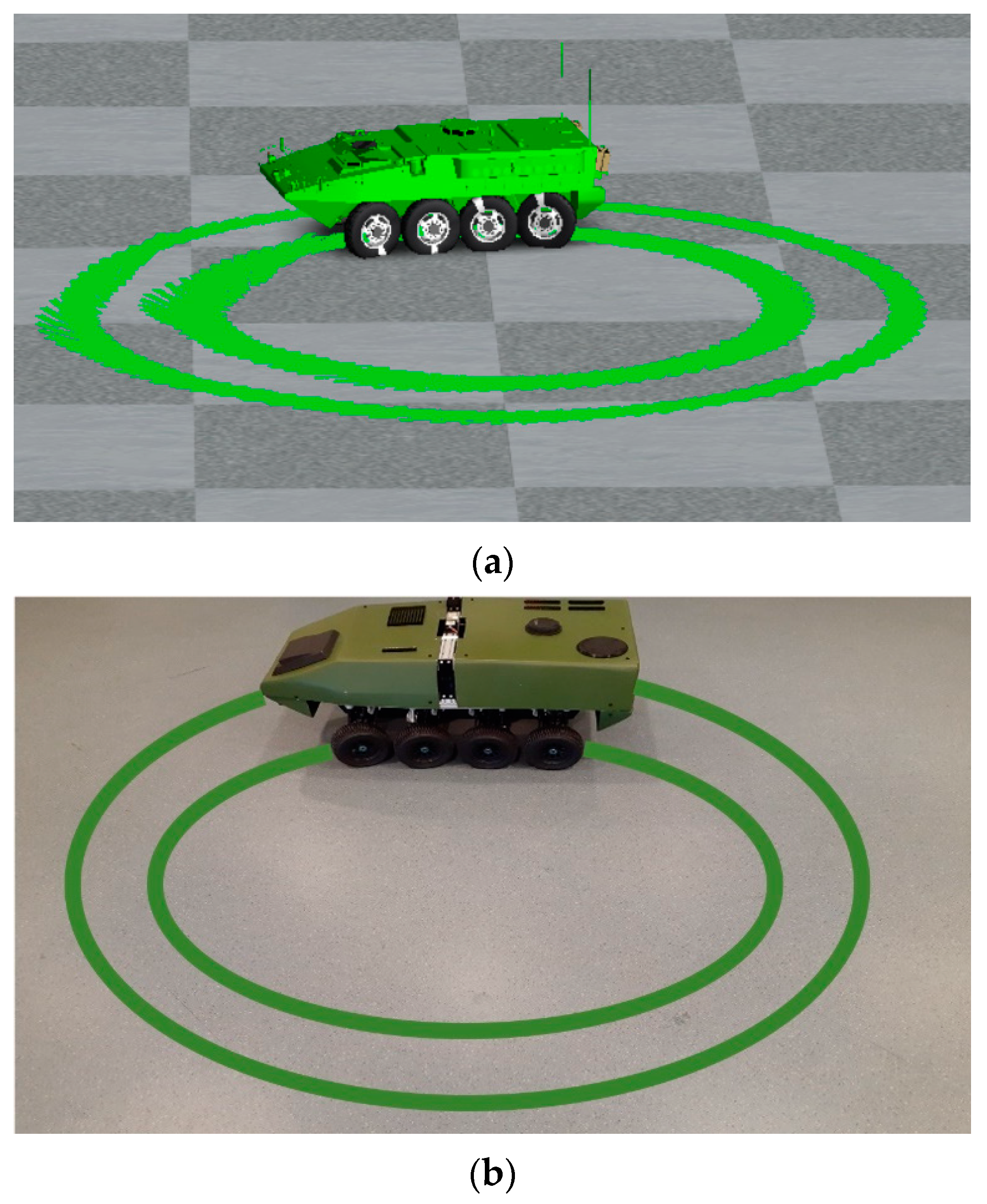
The turn radius evaluation’s physical and virtual versions are shown in Figure 11a,b. Figure 11a,b illustrate the scaled vehicle driven with a left turn in a circle path. During a turning maneuver, the 1st axle inner wheel always has the largest angle compared with the rest wheel’s angle based on the Ackermann condition equation, including Equations (3), (10) and (16). For that reason, the 1st axle’s inner wheel angle should not exceed the maximum wheel angle of the mechanical allowance. For instance, the eight wheels of the scaled vehicle have the same maximum mechanical allowance in terms of maximum steering wheel angle. Therefore, if the 1st axle’s inner wheel angle is steered under the maximum mechanical allowance, the remaining wheels’ angles should be under the maximum mechanical allowance. The scaled vehicle’s mechanical maximum steering wheel angle on each wheel is 24 degrees. However, during the turn radius evaluation, the 1st axle inner wheel angle is fixed at 20 degrees for safety reasons to prevent exceeding the maximum mechanical allowance. In the simulated turn radius evaluation, an angle of 20 degrees is allocated to the 1st axle inner wheel angle through open-loop steer control in TruckSim. On the other hand, in the physical turn radius evaluation, an angle of 20 degrees is set to the maximum steering input through Arduino codes. For example, an angle of 20 degrees is sent to the 1st axle inner wheel angle through the remote controller and the Arduino control system during turn radius evaluation.
The 1st axle inner wheel angles of the scaled vehicle in three different steering scenarios during turn radius evaluation are represented in Figure 12. The average of the 1st axle inner wheel angles from both experimental and simulation results are shown in Table 1. Table 1 is used to show the validation of simulation data compared with the experimental data in terms of the 1st axle inner wheel angles. The 1st axle inner wheel angles always have the largest values among the eight wheels; therefore, the 1st axle inner wheel angles are chosen to be shown in this study. The average values of the 1st axle left wheel angles in experimental data among three different scenarios show very slight differences due to the limitation of linear actuator sensors, but they are within the acceptable range of errors. The average of the 1st axle inner wheel angles in simulation data is set to be close to the average of experimental data by adjusting open-loop steer control in TruckSim for validation purposes. Maneuvering the scaled vehicle during turn radius evaluation in both experimental and simulation tests is very simple, as the steering input is the fixed values.
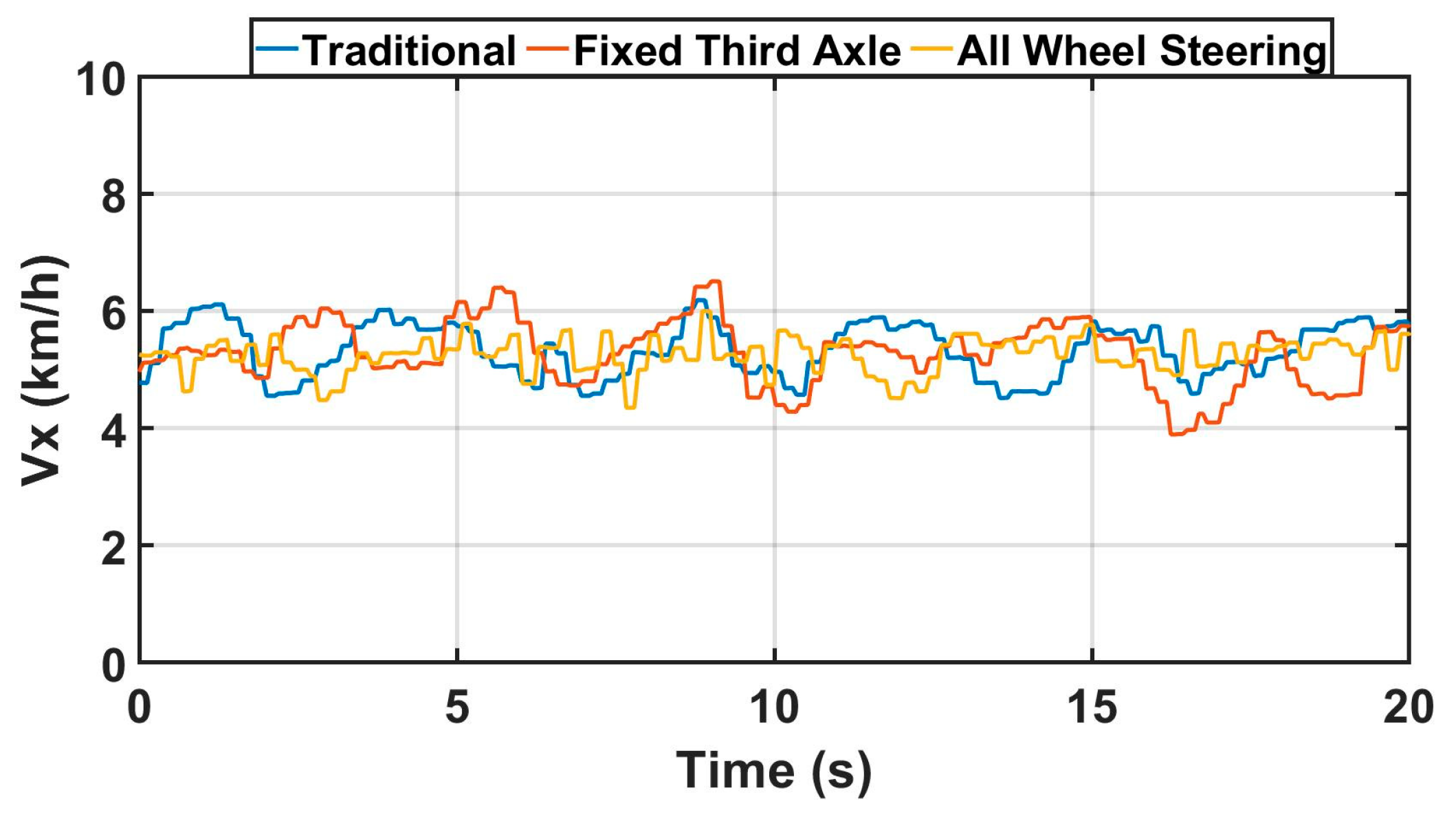
Figure 13 represents the experimental result of maximum velocity. Table 2 shows the average maximum velocity of the experimental and simulation data. Acquiring the same number of velocities, especially in experimental tests, is very important to compare the scale vehicle’s vehicle dynamics behaviors among three different steering scenarios. For instance, the average maximum velocities of three different steering modes in experimental data are very similar. These results also prove the mathematical model of scaled vehicles, since the variable eight-wheel speeds are designed and implemented to maintain the desired longitudinal velocity of the scale vehicle. In other words, having the same average maximum velocities indicates the continuous control of the variable eight-wheel speeds is working properly during turn radius evaluation. However, some fluctuations of experimental data in maximum velocity are observed due to the noise caused by GPS. For that reason, Table 2 (the average value of maximum velocity) is created to prove that three different scenarios have the same results of maximum velocity. The average maximum velocity in simulation data is selected to match with the average values of experimental data for validation by adjusting the constant target forward speed in TruckSim. In conclusion, both the experiments’ and simulation’s average maximum velocity show very similar numbers. In future studies, introducing GPS that has less noise level during turn radius evaluation will lead to a reduction in the fluctuation in experimental data.
The yaw rate is one of the turn radius evaluation outputs with two input components including maximum speed and maximum steering. The process of achieving maximum speed and maximum steering is explained above. Figure 14 illustrates the experimental result of the yaw rate with three different scenarios in turn radius evaluation. Table 3 explains the average yaw rate of the experimental and simulation data. In Table 3, the similar average yaw rates between simulation and experimental data at each steering scenario are shown for validation purposes. For instance, the difference between simulation and experimental results in traditional, fixed 3rd axle, and all-wheel steering scenarios represent 3%, 0.6%, and 2.3%, respectively. However, minor fluctuations of experimental data in terms of yaw rate in Figure 14 are seen due to the noise generated by IMU. Therefore, Table 3 is used to represent the average yaw rate of experimental data compared with simulation data that has no fluctuation.
Lateral acceleration is also one of the important output results to analyze the scaled vehicle dynamic performance. Moreover, lateral acceleration data are used to obtain and verify vehicle sideslip based on Equations (20) and (21). The process will be addressed in the next paragraph. Figure 15 shows the experimental result of lateral acceleration among three different steering modes in turn radius evaluation. For example, all-wheel steering has the highest value, as it has the smallest turn radius. The results of the turn radius evaluation will be explained more in the next paragraph. Table 4 indicates the average lateral acceleration in both the experimental and simulation data for the validation since the experimental result of lateral acceleration experiences fluctuations due to the noise of the IMU sensor. Table 4 shows very minor differences between experimental and simulation results in all three scenarios. For instance, the different percentages of simulation and experimental data in traditional, fixed 3rd axle, and all-wheel steering scenarios are 6.2%, 3.6%, and 0.9%, respectively.
a y s e n s o r = v ˙ y +   v x θ ˙
β ˙ = v ˙ y v x
In Equations (20) and (21), a y s e n s o r , v ˙ y , v x , θ ˙ , and β ˙ represent the lateral acceleration measured by IMU, lateral velocity change, longitudinal velocity, yaw rate, and vehicle sideslip change, respectively. The experimental and simulated data of lateral acceleration measured by IMU, longitudinal velocity, and yaw rate in turn radius evaluation were shown previously in Figure 13, Figure 14 and Figure 15 and Table 2, Table 3 and Table 4. Therefore, lateral velocity change can be obtained from Equation (20). In addition, vehicle sideslip change can be calculated by Equation (21) based on lateral velocity change and constant longitudinal velocity. Table 2, Table 3 and Table 4 demonstrate that the experimental and simulation results have similar data in terms of longitudinal velocity, yaw rate, and lateral acceleration. In conclusion, vehicle sideslip of the TruckSim simulation data is validated from experimental data and can be used to interpret the scaled vehicle’s dynamic behavior. For instance, Table 5 indicates the average vehicle sideslip obtained by the TruckSim simulation in turn radius evaluation. In Table 5, the traditional mode has the largest degree of vehicle sideslip, and the fixed 3rd axle has the smallest value. In addition, the all-wheel steering mode has a slightly lower vehicle sideslip than the traditional mode.
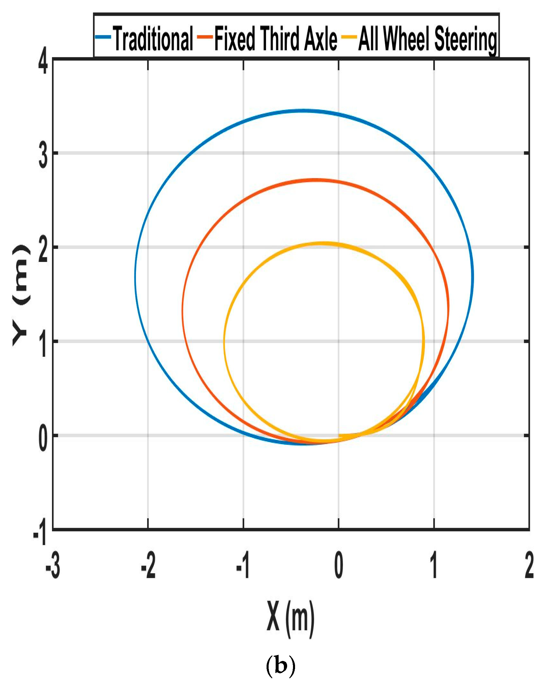
Figure 16 shows trajectory results from both the experiments and simulations regarding turn radius evaluation. Figure 16a shows values obtained by indoor GPS, and Figure 16b contains values generated by TruckSim. In Figure 16, the all-wheel steering scenario has the smallest turn radius compared to the other scenarios. These results can be verified by Equations (2), (9) and (15). For instance, L 1 of the traditional scenario has the largest value by the mathematical model design mentioned above, and δ i 1 (1st axle inner angle) and B (track width) have the same numbers in three different scenarios. Furthermore, in Figure 16, both experimental and simulated results have similar shapes and radii. For that reason, it is concluded that the simulation trajectory data are validated with the experimental trajectory data. The average radius of the experimental and simulated trajectory is described in Table 6.
R = V θ ˙
Figure 17a shows the turn radius calculated from the experimentally measured velocity and yaw rate based on Equation (22). In Equation (22), V and θ ˙ represent the maximum velocity and yaw rate shown in Figure 13 and Figure 14. The average value of Figure 17a is represented by Table 6. On the other hand, Figure 17b represents the turn radius calculated from the experimentally measured 1st axle inner angle based on Equations (2), (9) and (15). However, the turn radius of Figure 17b indicates a theoretical value that does not correspond to lateral skid. For instance, the average turn radius of Figure 17b shown in Table 6 has smaller values in three different scenarios. This phenomenon is strongly severe in the traditional mode due to the lateral skid caused by the fixed steering wheel on the 3rd and 4th axle. The differences in turn radius between indoor GPS and Figure 17b in traditional, fixed 3rd-axle, all-wheel are 17.3%, 8.3%, and 3%, respectively. These numbers explain the advantages of applying the all-wheel steering scenario compared to the traditional scenario during turn radius evaluation. Moreover, the all-wheel steering scenario has another advantage compared to the traditional scenario. Within the same mechanical maximum steering angle among eight steering wheels, 20 degrees, the turn radius of the all-wheel steering scenario is only 57.47% of that of the traditional scenario.

3.3. Double Lane Change Evaluation

Double lane change (DLC) evaluation is used to analyze the vehicle dynamics on rough surfaces and to validate the test results between the experimental and simulation data in three different steering scenarios. The test is validated in three different steering cases including traditional, fixed-third axle, and all-wheel steering. The scaled vehicle is evaluated virtually and physically through the DLC maneuver test to analyze various parameters. The parameters include the 1st axle left wheel angle, yaw rate, longitudinal velocity, trajectory, turning radius, and vehicle sideslip. Using the DLC maneuver test for both experiments and simulations, the simulation results of TruckSim can be validated with the experimental results within small errors. In DLC evaluation, a right-turning maneuver is represented as a negative number, and a left-turning maneuver is represented as a positive number in all figures.

Double Lane Change at 5 km/h

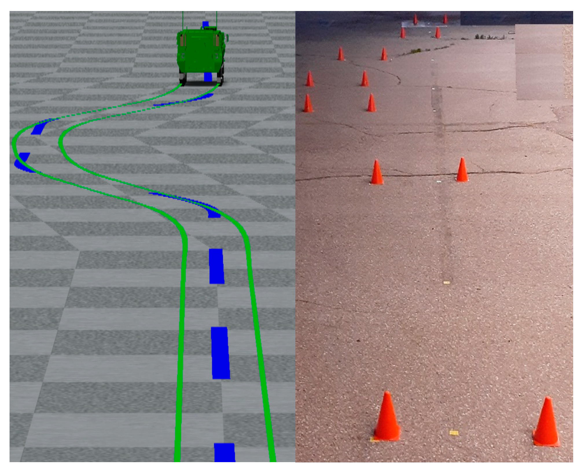
DLC’s physical and virtual evaluation are shown in Figure 18, and DLC’s dimension is explained in Figure 19. The desired driving path is calculated from the average value between inner and outer cones shown in Figure 19. The desired driving path shown in the blue dashed line in Figure 18 is implemented to run closed-loop driver model in TruckSim. In the physical DLC test, the driver is maneuvering the scaled vehicle to follow the trajectory results of TruckSim simulation by referring to cones. Therefore, driving the scaled vehicle physically on the same trajectory with the TruckSim simulation result is very important for validation between experiment and simulation. For instance, Figure 20 shows how similar trajectories are obtained between the experiments and simulations.
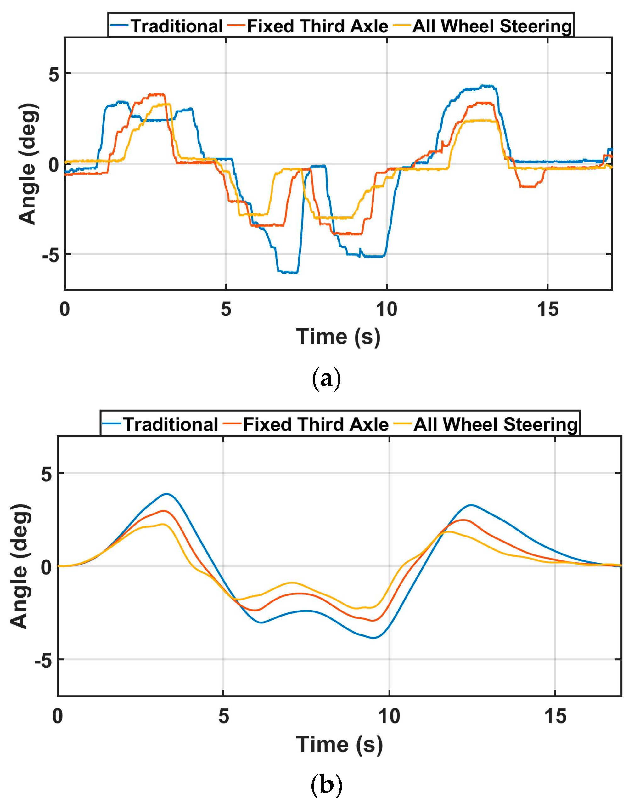
The scaled vehicle’s 1st axle left wheel angles in three different steering scenarios during the DLC evaluation are shown in Figure 21 to validate the simulated results with the experimentally obtained results. The 1st axle left wheel angles are selected in Figure 21 as they have the largest wheel angles during the left turn. Figure 21 shows quite similar positive and negative peak value times; however, some different amplitudes between the simulations and experiments are seen in negative values from 5 to 10 s. There are some difficulties for human drivers to maneuver the scaled vehicle like using a closed-loop driver model. In future research, the path following the closed-loop driver model will be implemented on the physically scaled vehicle to achieve the same trajectory of the simulation result. In both the experimental and simulation results of Figure 21, the all-wheel steering figure is the most shifted to the left compared to others between 5 and 15 s. This phenomenon indicates that all-wheel steering has the fastest response in three scenarios.
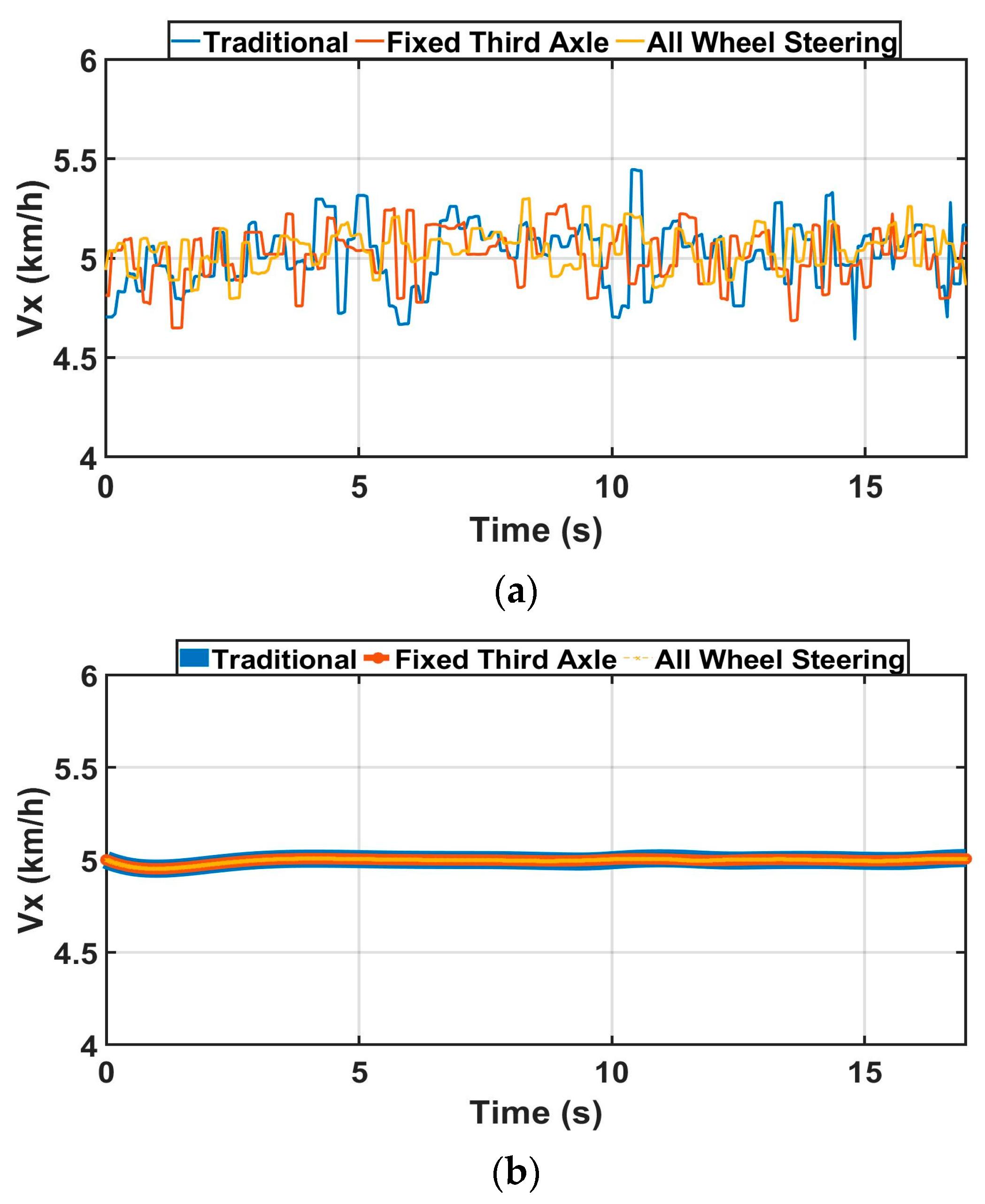
Figure 22 represents the longitudinal speed of the experimental and simulated data during the DLC evaluation at 5 km/h. Table 7 represents the average longitudinal speed of the experiment and simulation data from Figure 22. Achieving the same velocity in the three different scenarios is also one of the main required conditions in this study to analyze the vehicle dynamic performance among three different scenarios. For example, the average velocities of experiment data in three different scenarios are almost the same in Table 7 even though fluctuations are observed in Figure 22a. The fluctuations of experimental data are caused by the noise generated by GPS, and the range of the error in GPS is up to 0.3 km/h. However, the velocity of simulated data shows minor fluctuations caused by cornering performance. In conclusion, the average velocity values of both experimental and simulation results are almost the same, which can be used for one of the validations between simulation and experiment data. In future research, implementing a more accurate and robust GPS on the scaled vehicle can be conducted to minimize the fluctuation in experimental data.
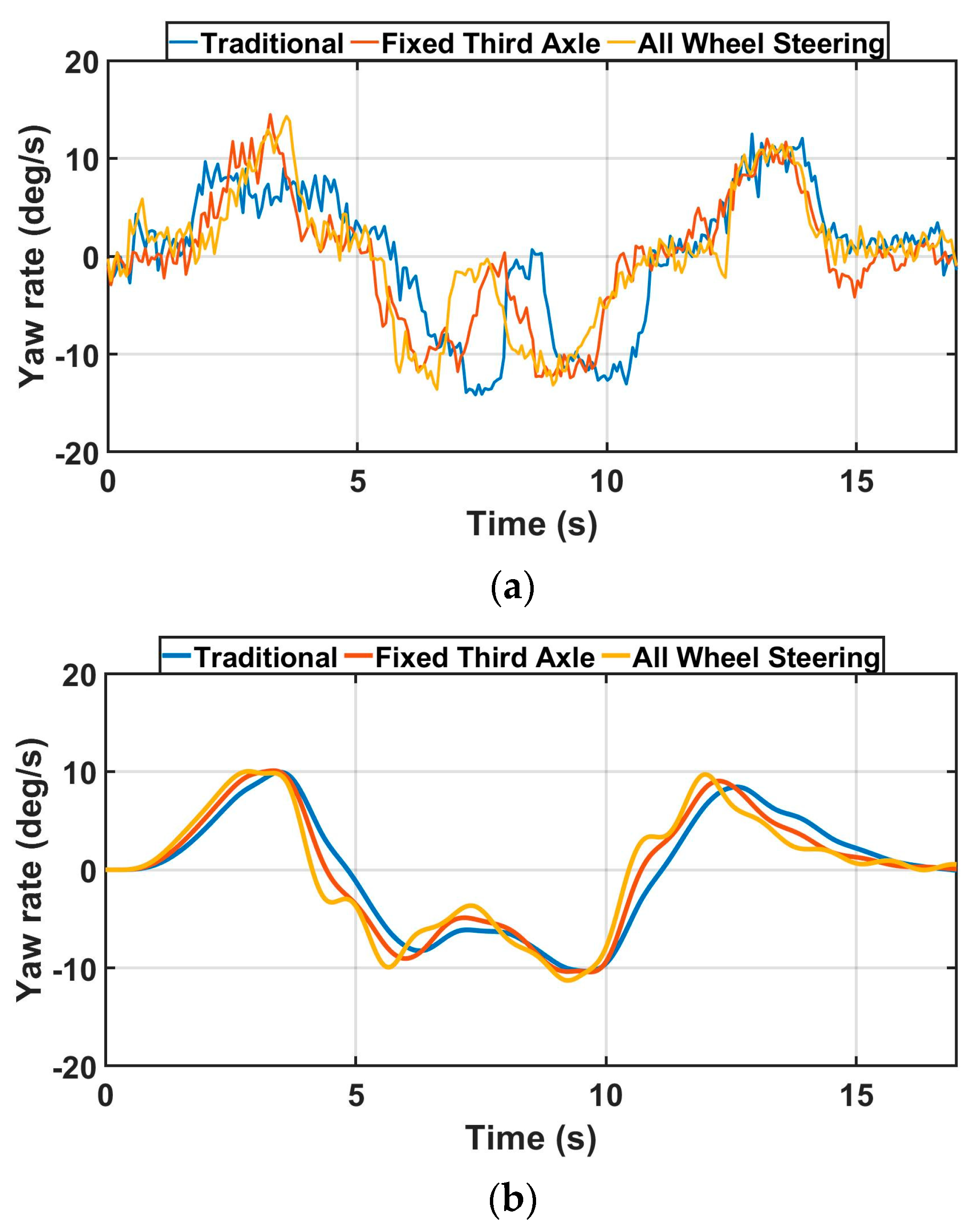
Figure 23 explains the yaw rate of experimental and simulated data during the DLC evaluation at 5 km/h. In general, the similar amplitude and peak value time in three different scenarios are shown in the experimental yaw rate result. However, there are some different shapes observed between 7 and 10 s in the experimental yaw rate result due to the slightly different trajectory of Figure 20a. In contrast to the experimental result, the simulation result of the yaw rate shows almost the same shapes as they have almost the same trajectory and velocity. This is the required condition in this research to evaluate the vehicle dynamic performance among three different steering scenarios. As mentioned earlier, implementing a path following a closed-loop driver model on the physically scaled vehicle will enhance the controllability of maneuvering the scaled vehicle especially in traditional steering mode. Consequently, the error of yaw rate and trajectory especially in traditional steering scenarios will be decreased. Furthermore, in both the experimental and simulation results of Figure 23, the all-wheel steering figure is slightly shifted to the left compared to others. This is evidence that the all-wheel steering scenarios have the fastest response compared to others regarding the same driving strategies (closed-loop driver model in TruckSim and human driving with remote control).

4. Discussion

In this section, the most significant results including turn radius and vehicle sideslip in DLC evaluation are introduced to highlight the goal of this study.

Analysis of Turn Radius and Vehicle Sideslip in Double Lane Change Evaluation

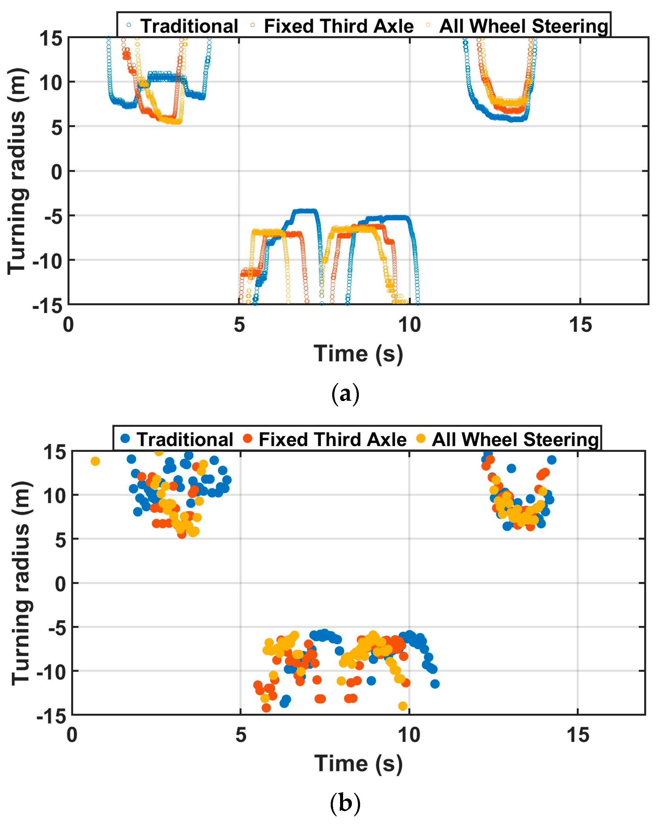
Figure 24 shows two types of turning radius during the DLC maneuver at a speed of 5 km/h. Figure 24a represents the turning radius calculated from the experimental 1st axle left angle data of Figure 21a by using Ackermann condition equations such as Equations (2), (9) and (15). Figure 24a shows the theoretical turning radius not reflecting tire slip and lateral skid. However, Figure 24b shows the actual turning radius calculated from experimental velocity (Figure 22a) and experimental yaw rate (Figure 23a) by applying Equation (22). In other words, Figure 24b, the actual turning radius, reflects tire slip and lateral skid. In Figure 24b, the amplitude of the turning radius in three different scenarios has the same amount from 5 to 15 s. This is confirmed with the experimental trajectory results mentioned previously, as three scenarios show similar trajectories in Figure 20. In contrast to Figure 24b, Figure 24a shows that the traditional steering scenario has a lower turning radius compared to the other two scenarios from 5 to 15 s, which is caused by higher lateral skid due to the design of Ackermann steering design in Figure 4. This is one of the disadvantages of the traditional steering scenario, as the scaled vehicle uses extra steering input effort in the traditional steering scenario.
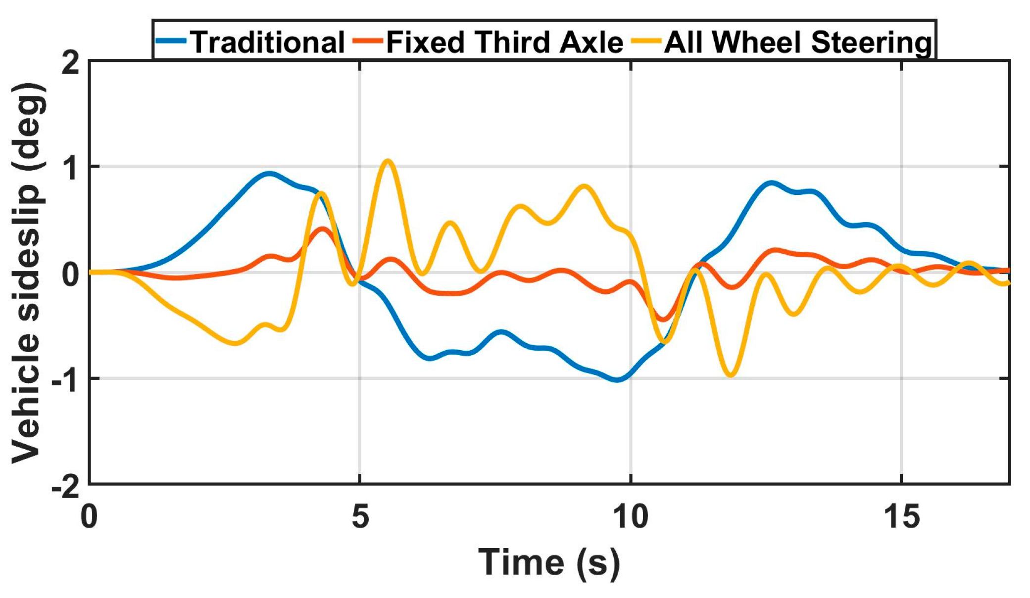
Figure 25 shows vehicle sideslip from TruckSim simulation results in three different scenarios. In Figure 25, the fixed third axle scenario experiences minimal amplitude; however, traditional and all-wheel steering scenarios show a relatively larger amount of vehicle sideslip. Therefore, the fixed third axle scenario has the most advantage in terms of the vehicle sideslip aspect of vehicle dynamic, since it has the least amplitude during the DLC maneuver test. Moreover, all-wheel steering is still acceptable in terms of the vehicle sideslip aspect because all-wheel steering has a similar level of amplitude to the traditional mode.

5. Conclusions

In the research paper, three real-world experiments such as stationary evaluation, turn radius evaluation, and double lane change evaluation are conducted to validate the scaled vehicle’s TruckSim simulated data by comparing with the experimental data in terms of vehicle dynamic performance among three different steering scenarios. The Ackermann steering strategy mentioned in this study is implemented on the 8 × 8 scaled electric combat vehicle.
In stationary evaluation, the error between the simulation data and experimental data is very minor in general among three different steering scenarios, which indicates that the desired eight-wheel velocities are applied to the scaled vehicle correctly. Moreover, to implement an all-wheel steering scenario on the scaled vehicle, a higher maximum speed for the eight wheels is required to meet the vehicle’s mathematical model compared to the traditional steering scenario.
In turn radius evaluation, almost the same maximum velocity within three different scenarios demonstrates that the continuous variable eight-wheel speeds strategy is working properly to maintain the desired longitudinal velocity. The all-wheel steering mode is still acceptable until 5.3 km/h compared to the traditional mode with respect to the vehicle sideslip. However, minor fluctuations of experimental data in terms of yaw rate and lateral acceleration are seen due to the noise generated by IMU. Because of these noises, the experimental vehicle sideslip result is not able to be calculated. Utilizing a high-performance IMU that can work without noise around 5 km/h will be investigated in future work to obtain experimental vehicle sideslip results. The turn radius calculated from the experimentally measured 1st axle inner angle based on the Ackermann condition equation is smaller than the measured turn radius of indoor GPS especially in the traditional steering scenario. This is because of the lateral skid caused by the fixed steering wheel on the 3rd and 4th axle. However, this phenomenon is much less severe in an all-wheel steering scenario. For example, the errors in terms of turn radius between the indoor GPS and the experimental result calculated from the measured 1st axle inner angle (steering input effort) in traditional, fixed 3rd-axle, and all-wheel modes are 17.3%, 8.3%, and 3%, respectively. These figures indicate the benefits of applying the all-wheel steering scenario compared to the traditional scenario. Within the same mechanical maximum steering angle among eight steering wheels, 20 degrees, the turn radius of the all-wheel steering scenario is only 57.47% that of the traditional scenario. This will enhance the 8 × 8 combat vehicle’s survivability and operation ability during a battle.
In double lane change evaluation, 1st axle left wheel angles and yaw rate in three different steering scenarios between experimental and simulated data show quite similar shapes. However, some different peak values between simulation and experiment are observed. These different peak values are caused by human drivers’ errors, as the driver is not able to maneuver the scaled vehicle in the same manner as TruckSim’s closed-loop driver model. For that reason, in future research, the path following the closed-loop driver model will be developed to be installed on the physically scaled vehicle through Robot Operating Software to obtain the same trajectory of the simulation result. The 1st axle left wheel angle and yaw rate in the all-wheel steering scenario in both experimental and simulated data are slightly shifted to the left compared to the other scenarios. This represents that the all-wheel steering mode has the fastest response to the steering input. The two types of experimental results of turning radius are shown to evaluate the lateral skid during cornering among three different steering scenarios. The differences between the two types of results indicate the amount of lateral skid. For instance, the traditional steering scenario shows the largest difference between two different turning radius results. In contrast, the all-wheel steering scenario represents the minimum error between two different turning radius results. Consequently, the all-wheel steering scenario has a smaller lateral skid than the traditional steering scenario. In addition to that, the fixed third axle scenario has the most advantage in terms of vehicle sideslip. All-wheel steering is still acceptable since it has a similar level of vehicle sideslip to traditional.

Author Contributions

Conceptualization, J.K. and M.E.-G.; methodology, J.K.; software, J.K. and Z.E.-S.; validation, J.K., M.E.-G. and Z.E.-S.; formal analysis, J.K. and M.E.-G.; investigation, M.E.-G.; resources, J.K.; data curation, J.K.; writing—original draft preparation, J.K.; writing—review and editing, J.K., M.E.-G., and Z.E.-S.; visualization, J.K.; supervision, M.E.-G. and Z.E.-S.; project administration, M.E.-G.; funding acquisition, M.E.-G. and Z.E.-S. All authors have read and agreed to the published version of the manuscript.

Funding

This research received no external funding.

Data Availability Statement

Data are contained within the article.

Acknowledgments

The authors express their gratitude would like to the Natural Sciences and Engineering Research Council of Canada (NSERC Discovery Grant) for their continuous support during the course of this study.

Conflicts of Interest

The authors declare no conflict of interest.

Appendix A

Table A1. The definition of variables.
R (m) Turning radius
L1 (m)The shortest distance from point C to the first axle
L2 (m)The shortest distance from point C to the second axle
L3 (m)The shortest distance from point C to the third axle
L4 (m)The shortest distance from point C to the fourth axle
B (m)Track width
rt (m)The radius of tire
θt (rad)The steering wheel angle
θ ˙ (rad/s)Yaw
δoj (rad)Each axle’s outer wheel angle
δij (rad)Each axle’s inner wheel angle
V (m/s)Longitudinal velocity
a y s e n s o r (g)Lateral acceleration measured by IMU
v ˙ y (g)Lateral velocity change
β ˙ (rad/s)Vehicle sideslip change

References

  1. Selmanaj, D.; Corno, M.; Sename, O.; Savaresi, S. Advantages of rear steer in LTI and LPV vehicle stability control. In Proceedings of the 52nd IEEE Conference on Decision and Control, Firenze, Italy, 10–13 December 2013; pp. 3523–3528. [Google Scholar] [CrossRef]
  2. D’Urso, P. Development of H∞ Control Strategy for a Multi-Wheeled Combat Vehicle. Ph.D. Thesis, University of Ontario Institute of Technology, Oshawa, ON, Canada, 2016. [Google Scholar]
  3. Zhang, Z.; Du, H.; Chen, S.; Li, Y.; Wang, H. A novel electro-hydraulic servo steering system for Ackermann steering of the heavy multi-axle vehicle. Proc. Inst. Mech. Eng. Part D J. Automob. Eng. 2022, 236, 2610–2624. [Google Scholar] [CrossRef]
  4. Ma, F.; Shi, J.; Yang, Y.; Li, J.; Dai, K. ACK-MSCKF: Tightly-Coupled Ackermann Multi-State Constraint Kalman Filter for Autonomous Vehicle Localization. Sensors 2019, 19, 4816. [Google Scholar] [CrossRef] [PubMed]
  5. Yu, Z.; Wang, J. Simultaneous Estimation of Vehicle’s Center of Gravity and Inertial Parameters Based on Ackermann’s Steering Geometry. J. Dyn. Syst. Meas. Control 2017, 139, 031006. [Google Scholar] [CrossRef]
  6. Girbacia, T.M.; Mogan, G.L. Velocity Variation Analysis of an Autonomous Vehicle in Narrow Environment. In New Advances in Mechanism and Machine Science; Springer: Berlin/Heidelberg, Germany, 2018; pp. 301–308. [Google Scholar] [CrossRef]
  7. Ataei, M.; Khajepour, A.; Jeon, S. Model predictive control for integrated lateral stability, traction/braking control, and rollover prevention of electric vehicles. Int. J. Veh. Mech. Mobil. 2019, 58, 49–73. [Google Scholar] [CrossRef]
  8. Aboelfadl, A.M. Integrated Chassis Control Strategies for Multi-Wheel Combat Vehicle. Ph.D. Thesis, Ontario Tech University, Oshawa, ON, Canada, 2021. [Google Scholar]
  9. Zhang, J.; Zhou, S.; Li, F.; Zhao, J. Integrated nonlinear robust adaptive control for active front steering and direct yaw moment control systems with uncertainty observer. Trans. Inst. Meas. Control. 2020, 42, 3267–3280. [Google Scholar] [CrossRef]
  10. Changoski, V.; Gjurkov, I.; Jordanoska, V. Improving vehicle dynamics employing individual and coordinated sliding mode control in vehicle stability, active front wheel steering and active rear wheel steering systems in co-simulation environment. In Proceedings of the IOP Conference Series: Materials Science and Engineering, Kragujevac, Serbia, 13–14 October 2022; IOP Publishing: Bristol, UK, 2022; Volume 1271, p. 012026. [Google Scholar]
  11. Zhou, X.; Wang, Z.; Wang, J. Automated ground vehicle path-following: A robust energy-to-peak control approach. IEEE Trans. Intell. Transp. Syst. 2021, 23, 14294–14305. [Google Scholar] [CrossRef]
  12. Samada, S.E.; Puig, V.; Nejjari, F. Robust TS-ANFIS MPC of an autonomous racing electrical vehicle considering the battery state of charge. IEEE ASME Trans. Mechatron. 2023, 28, 656–667. [Google Scholar] [CrossRef]
  13. Guevara, L.; Jorquera, F.; Walas, K.; Auat-Cheein, F. Robust control strategy for generalized N-trailer vehicles based on a dual-stage disturbance observer. Control Eng. Pract. 2023, 131, 105382. [Google Scholar] [CrossRef]
  14. Tan, A.H.; Peiris, M.; El-Gindy, M.; Lang, H. Design and development of a novel autonomous scaled multi-wheeled vehicle. Robotica 2022, 40, 1475–1500. [Google Scholar] [CrossRef]
  15. Available online: https://marvelmind.com/product/starter-set-super-mp-3d (accessed on 11 July 2023).
  16. RobotShop. UM7-LT Orientation Sensor. 2022. Available online: https://www.robotshop.com/ca/en/um7-lt-orientation-sensor.html (accessed on 20 June 2022).
  17. Locosys. MC-1513 GPS. 2022. Available online: https://www.locosystech.com/en/product/gnss-module-mc-1513-g.html (accessed on 22 May 2022).
  18. Logitech. F710 USB Controller. 2022. Available online: https://www.logitechg.com/en-ca/products/gamepads/f710-wireless-gamepad.940-000117.html (accessed on 10 May 2023).
  19. CUI Devices. AMT10 Rotary Encoders. 2022. Available online: https://www.cuidevices.com/product/motion/rotary-encoders/incremental/modular/amt10-series (accessed on 15 May 2022).
  20. Hobby Pros. Lipo Battery Gens Ace 6200 mAh 14.8V 45C. 2022. Available online: https://www.hobbyprosdepot.com/product-p/ga-b-45c-6200-4s1p-deans.htm (accessed on 11 May 2023).
  21. Russell, B. Development and Analysis of Active Rear Axle Steering for 8 × 8 Combat Vehicle. Ph.D. Thesis, University of Ontario Institute of Technology, Oshawa, ON, Canada, 2018. [Google Scholar]
  22. Kim, J.; El-Gindy, M.; El-Sayegh, Z. Development of Novel Steering Scenarios for an 8 × 8 Scaled Electric Combat Vehicle; SAE International: Warrendale, PA, USA, 2023. [Google Scholar] [CrossRef]
Figure 1. Closed-loop controller of linear actuator [14].
Machines 12 00146 g001
Figure 2. Steering assembly.
Machines 12 00146 g002
Figure 3. Schematic diagram. (a) Driving systems [14]. (b) Suspension systems [14].
Machines 12 00146 g003
Figure 4. Mathematical model of traditional steering scenario [22].
Machines 12 00146 g004
Figure 5. Mathematical model of fixed third axle steering scenario.
Machines 12 00146 g005
Figure 6. Mathematical model of all-wheel steering scenario.
Machines 12 00146 g006
Figure 7. Stationary evaluation with tachometer.
Machines 12 00146 g007
Figure 8. Eight wheels’ velocities in the traditional scenario. (a) Experimental result [17]. (b) Simulation result [17].
Machines 12 00146 g008aMachines 12 00146 g008b
Figure 9. Eight wheels’ velocities in a fixed 3rd axle scenario. (a) Experimental result. (b) Simulation result.
Machines 12 00146 g009
Figure 10. Eight wheels’ velocities in an all-wheel scenario. (a) Experimental result. (b) Simulation result.
Machines 12 00146 g010
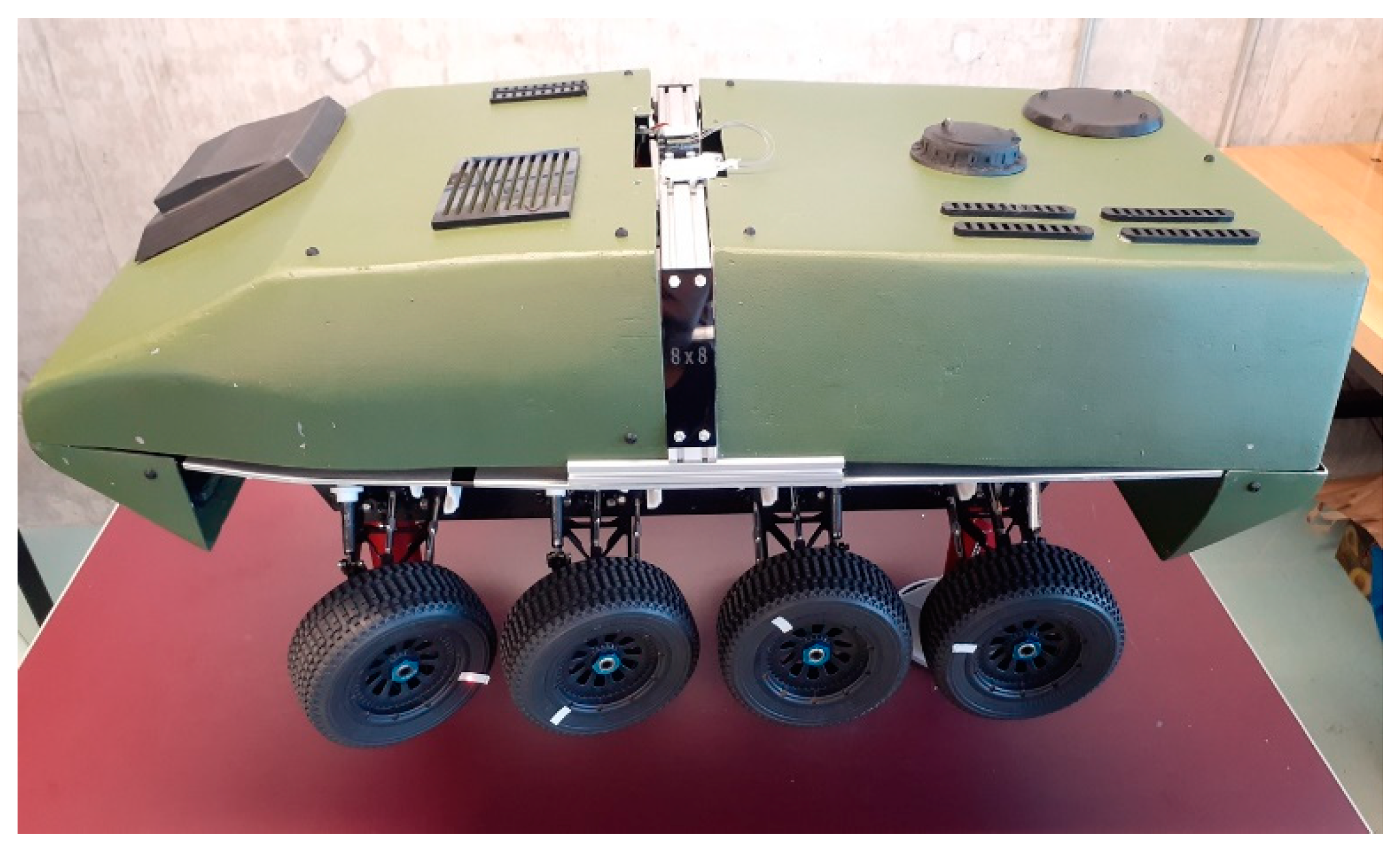
Figure 11. Turn radius evaluation. (a) Simulated scaled electric combat vehicle. (b) Physically tested scaled electric combat vehicle.
Machines 12 00146 g011
Figure 12. Experimental result of 1st axle inner wheel angles (turn radius evaluation at maximum speed and maximum steering).
Machines 12 00146 g012
Figure 13. Experiment result of maximum (velocity turn radius evaluation at maximum speed and maximum steering).
Machines 12 00146 g013
Figure 14. Experiment result of yaw rate (turn radius evaluation at maximum speed and maxi mum steering).
Machines 12 00146 g014
Figure 15. Experiment result of lateral acceleration (turn radius evaluation at maximum speed and maximum steering).
Machines 12 00146 g015
Figure 16. Result of trajectory (turn radius evaluation at maximum speed and maximum steering). (a) Experiment result. (b) Simulation result.
Machines 12 00146 g016aMachines 12 00146 g016b
Figure 17. Turn radius evaluation at maximum speed and maximum steering. (a) Experimental result of turning radius calculated from measured velocity and measured yaw rate. (b) Experimental result of turning radius calculated from measured 1st axle inner angle based on Ackermann condition equation.
Machines 12 00146 g017
Figure 18. Simulated scaled electric combat vehicle (left), and trajectory of the physically tested scaled electric combat vehicle (right) in double lane change evaluation.
Machines 12 00146 g018
Figure 19. Scaled double lane change setup.
Machines 12 00146 g019
Figure 20. Result of trajectory (DLC maneuver at a speed of 5 km/h). (a) Experiment result. (b) Simulation result.
Machines 12 00146 g020
Figure 21. Result of 1st axle left wheel angle (DLC maneuver at speed 5 km/h). (a) Experimental result. (b) Simulation result.
Machines 12 00146 g021
Figure 22. Result of longitudinal velocity (DLC maneuver at speed 5 km/h). (a) Experimental result. (b) Simulation result.
Machines 12 00146 g022
Figure 23. Result of yaw rate (DLC maneuver at speed 5 km/h). (a) Experimental result. (b) Simulation result.
Machines 12 00146 g023
Figure 24. Result of turning radius (DLC maneuver at speed 5 km/h). (a) Experimental result calculated from measured 1st axle left angle based on Ackermann condition equation. (b) Experimental result calculated from measured velocity and measured yaw rate.
Machines 12 00146 g024
Figure 25. Simulation result of vehicle sideslip.
Machines 12 00146 g025
Table 1. Average steering angle from 1st axle inner wheel angles.
TraditionalFixed 3rd AxleAll Wheel
Experimental result of 1st axle inner wheel angle (deg)20.5320.0020.14
Simulation result of 1st axle inner wheel angle (deg)20.519.8519.85
Table 2. The average of maximum velocity.
TraditionalFixed 3rd AxleAll Wheel
Experiment result of maximum velocity (km/h)5.295.255.24
Simulation result of maximum velocity (km/h)5.305.205.20
Table 3. The average yaw rate.
TraditionalFixed 3rd AxleAll Wheel
Experiment result of yaw rates (deg/s)47.8060.6378.68
Simulation result of yaw rates (deg/s)49.361.080.5
Table 4. The average lateral acceleration.
TraditionalFixed 3rd AxleAll Wheel
Experimental result of lateral acceleration (g)0.1370.1730.209
Simulation result of lateral acceleration (g)0.1290.1670.207
Table 5. The average vehicle sideslip angle.
TraditionalFixed 3rd AxleAll Wheel
Simulation result of vehicle sideslip angle (deg)4.81.4−3.9
Table 6. Average turn radius from different steering scenarios and measurement method.
TraditionalFixed 3rd AxleAll Wheel
Experiment result of trajectory from indoor GPS (m)1.741.331.00
Simulation result of trajectory from TruckSim (m)1.761.391.05
Experimental result of turning radius calculated from measured velocity and measured yaw rate (m)1.751.371.06
Experimental result of turning radius calculated from measured 1st axle inner angle based on Ackermann condition equation (m)1.441.220.97
Table 7. Average velocity (DLC maneuver at speed 5 km/h).
TraditionalFixed 3rd AxleAll Wheel
Experiment result (km/h)5.0145.0185.040
Simulation result (km/h)4.9954.9954.995
Disclaimer/Publisher’s Note: The statements, opinions and data contained in all publications are solely those of the individual author(s) and contributor(s) and not of MDPI and/or the editor(s). MDPI and/or the editor(s) disclaim responsibility for any injury to people or property resulting from any ideas, methods, instructions or products referred to in the content.