


Optimization of Machining Parameters for Reducing Drum Shape Error Phenomenon in Wire Electrical Discharge Machining Processes


Abstract
1. Introduction
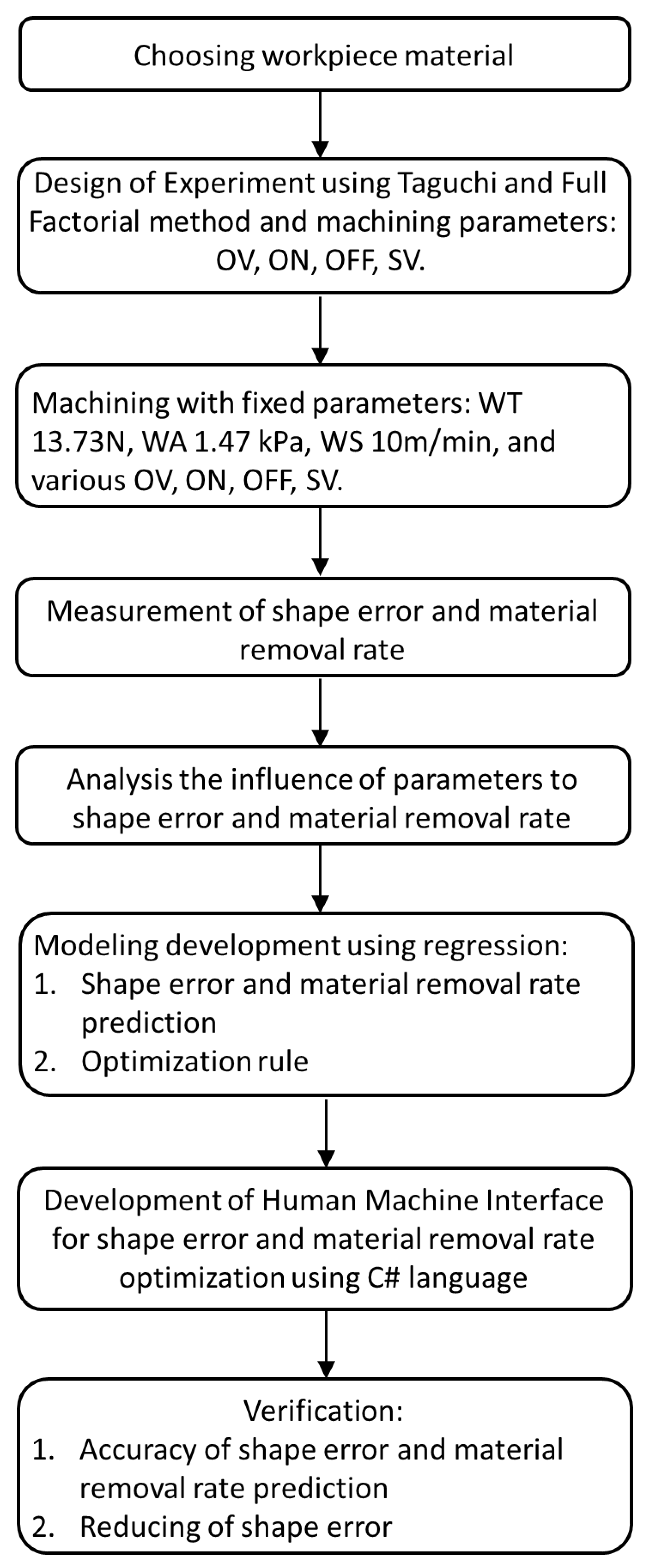
2. Methodology
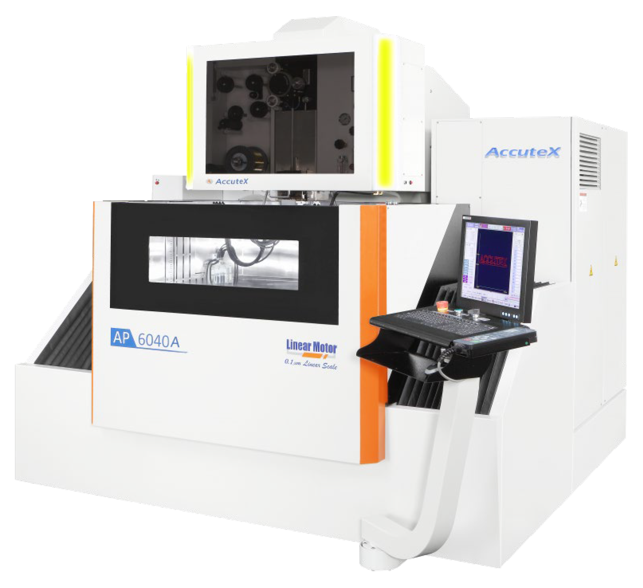
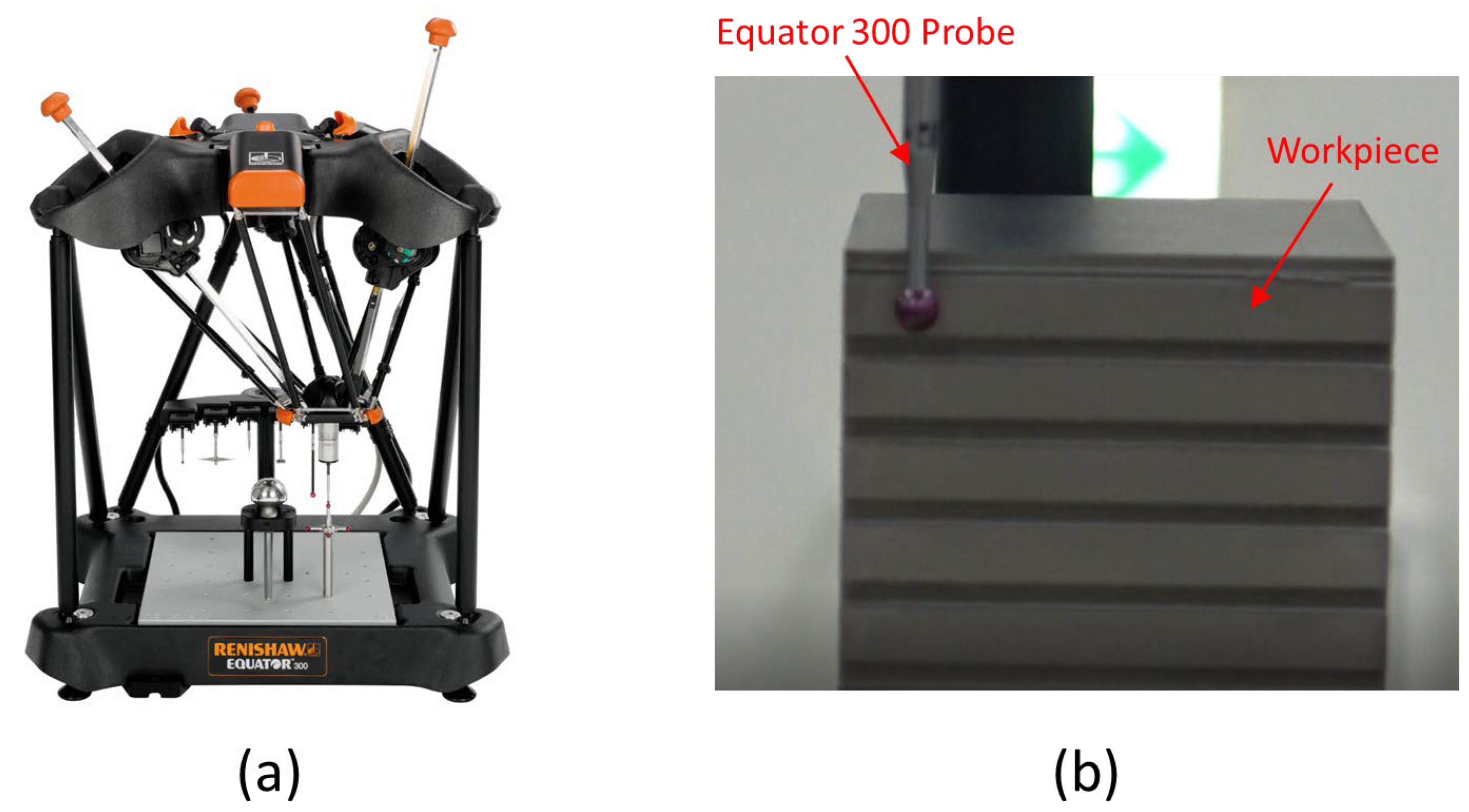
2.1. Experiment Design and Equipment
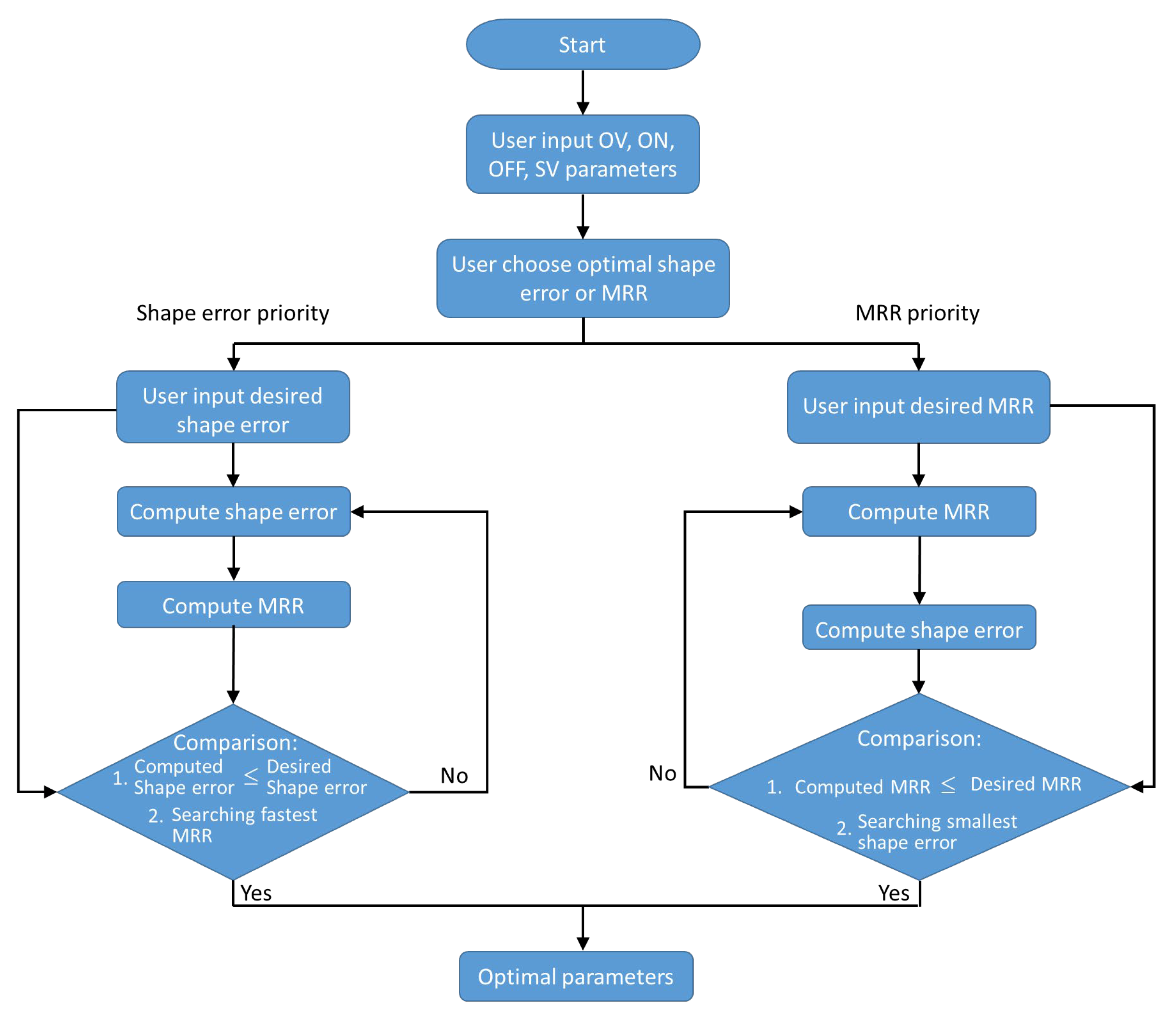
2.2. Optimization
- The user inputs the OV, ON, OFF, and SV parameter values.
- The user chooses the shape error or MRR priority.
- For shape error priority:
- (a)
- The user inputs the desired shape error.
- (b)
- Calculate the shape error using the equation for shape error prediction.
- (c)
- Calculate the MRR using the equation for MRR prediction.
- (d)
- Compare the shape error prediction value and the desired shape error value. If the predicted shape error value is ≥ the desired shape error value, return to step 3(b).If the predicted shape error value is ≤ the desired shape error value, proceed to step 3(e).
- (e)
- Search for the fastest machining while keeping the predicted shape error value ≤ the desired shape error value.
- (f)
- Optimal parameters are set.
- For MRR priority:
- (a)
- The user inputs the desired MRR.
- (b)
- Calculate the MRR using the equation for MRR prediction.
- (c)
- Calculate the shape error using the equation for shape error prediction.
- (d)
- Compare the MRR prediction value and the desired MRR value.If the predicted MRR value is ≥ the desired MRR value, return to step 4(b).If the predicted MRR value is ≤ the desired MRR value, proceed to step 4(e).
- (e)
- Search for the smallest shape error while keeping the predicted MRR value ≤ the desired MRR value.
- (f)
- Optimal parameters are set.
- Optimal parameters.
3. Experiment Result and Discussion
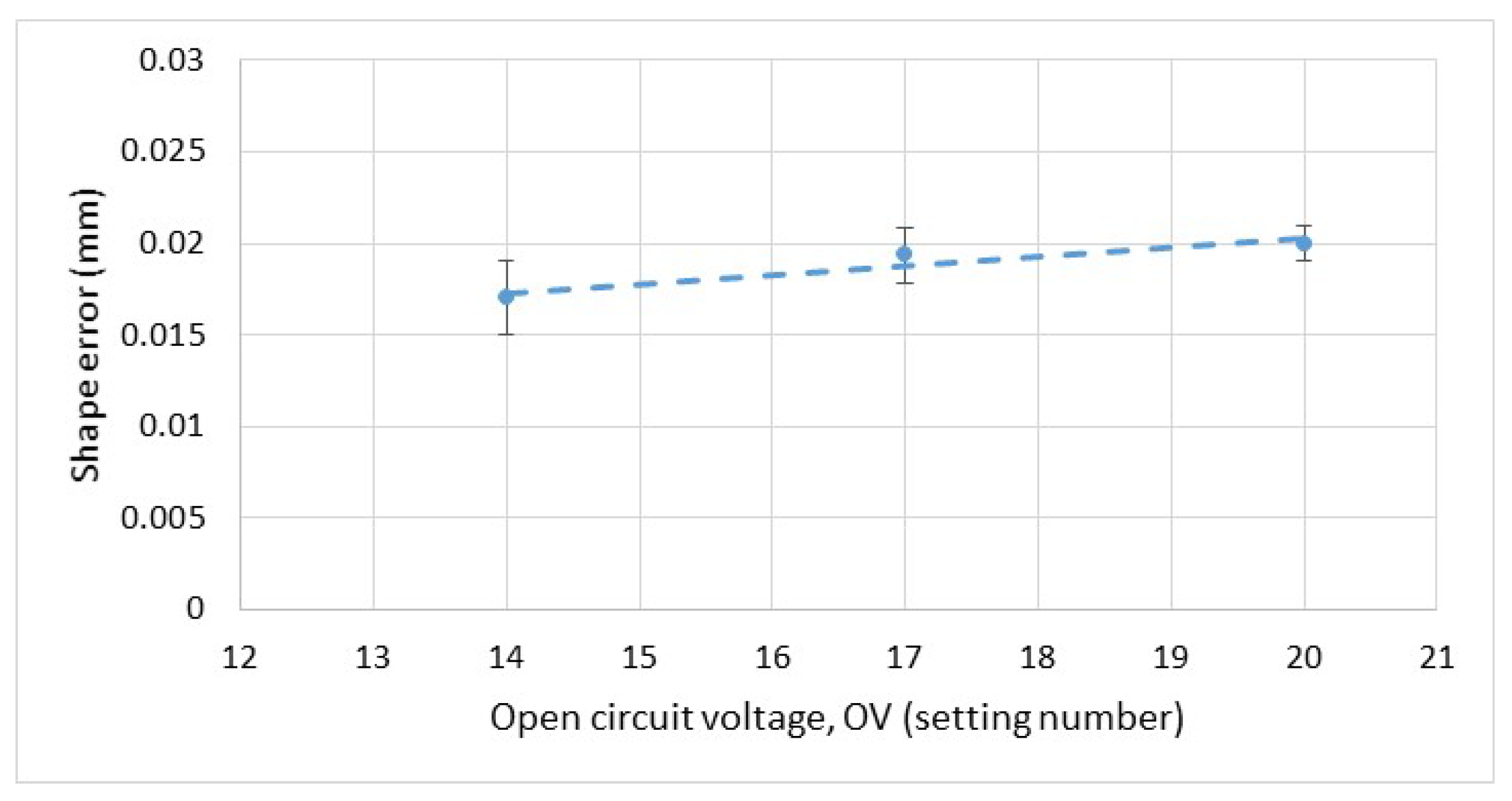
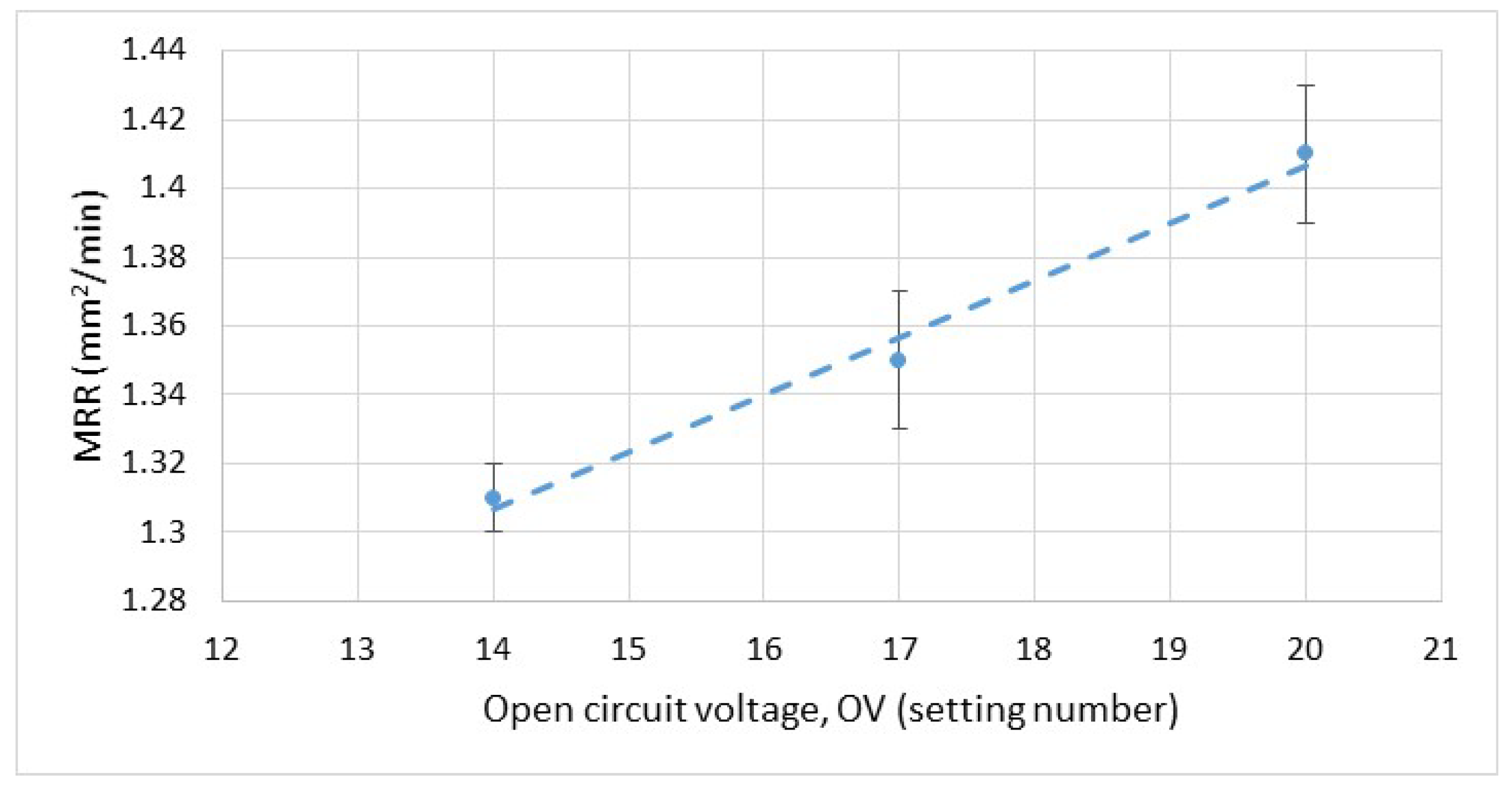
3.1. Effect of Open Circuit Voltage on Shape Error and MRR
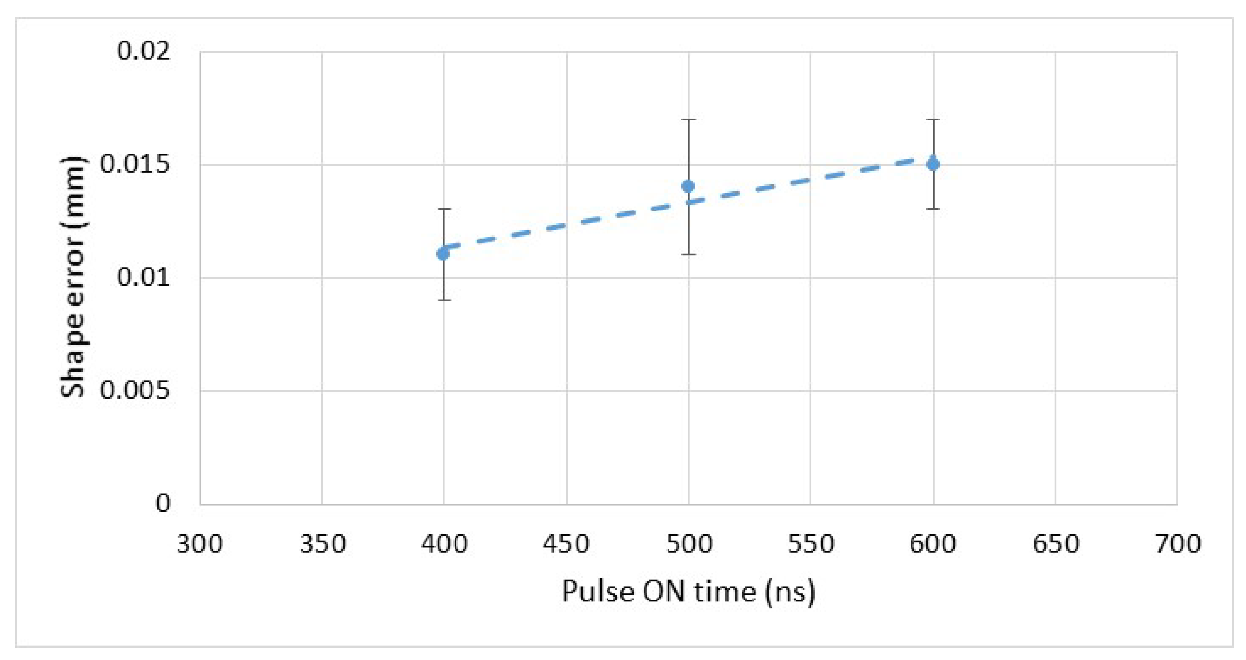
3.2. Effect of Pulse ON Time on Shape Error and MRR
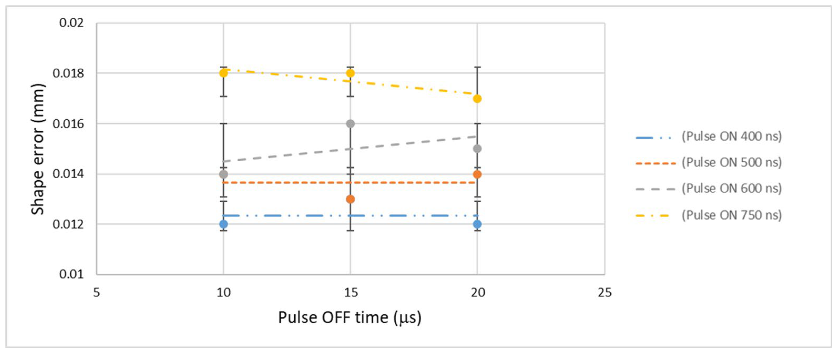
3.3. Effect of Pulse OFF Time on Shape Error and MRR
3.4. Effect of Servo Voltage on Shape Error and MRR
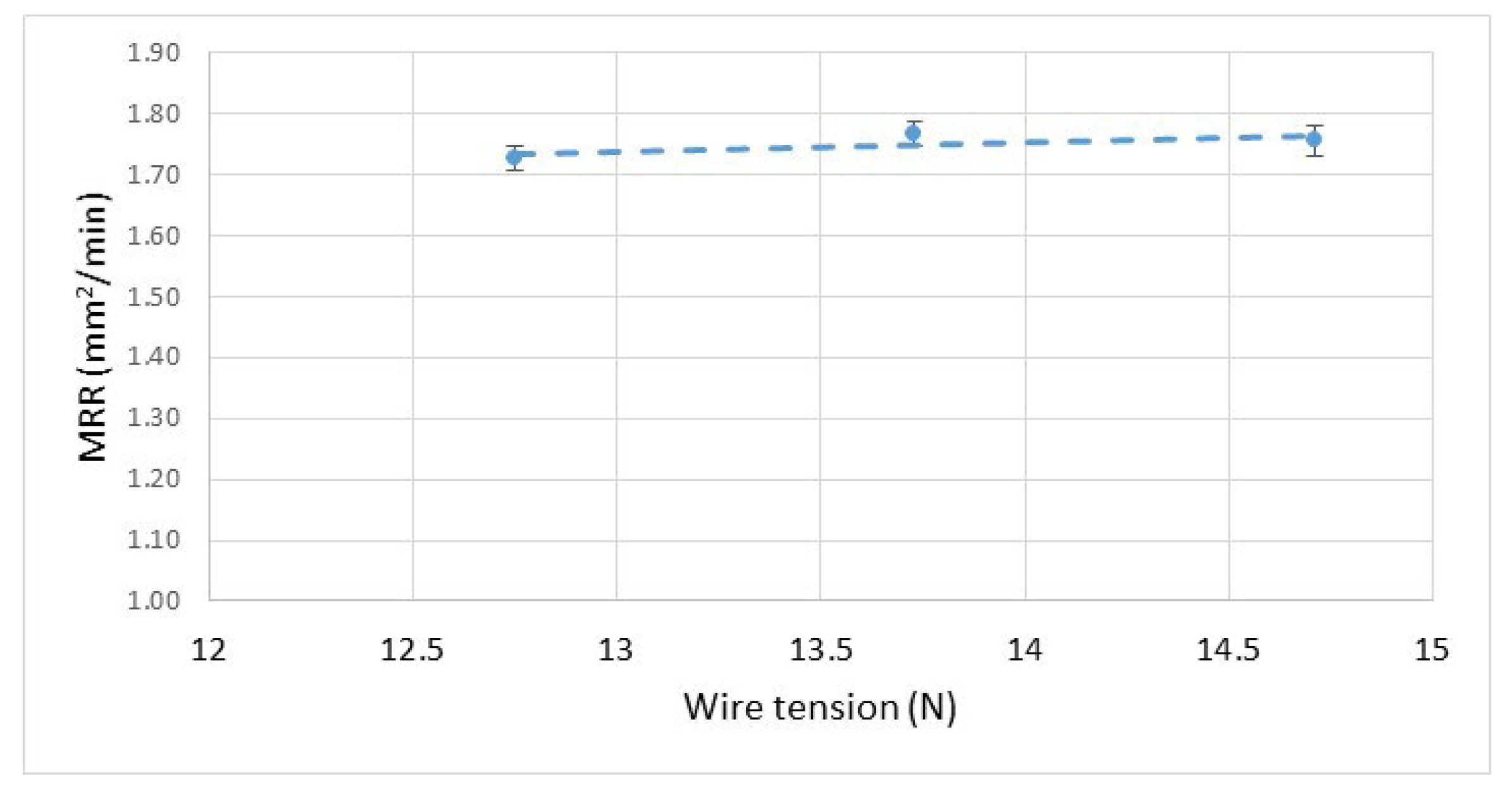
3.5. Effect of Wire Tension on Shape Error and MRR
3.6. Effect of Flushing Pressure on Shape Error
3.7. Prediction Modeling
4. Human–Machine Interface
- Prediction module: The first part focuses on predicting the shape error and MRR based on the parameters input by the user.
- Shape error optimization module: The second part calculates and searches the parameter combination that follows the optimization rules according to the user-required shaper error and then presents the results. Additionally, an estimation of the MRR is calculated using the optimized parameters.
- MRR optimization module: The third part calculates and searches the combination of parameters that follow the optimization rules according to the user-required MRR and then displays the results. Additionally, an estimation of the shape error is calculated using the optimized parameters.
- The user enters the parameter values into the corresponding parameter fields in area 1 (number 1 in Figure 18). Afterward, the user presses the “Shape error prediction” button to obtain the predicted shape error and MRR values for the current parameters.
- The user chooses the priority of optimization. If the user chooses shape error optimization as the priority, then proceed to step three. If the user chooses MRR as the priority, then proceed to step four.
- The user enters the desired shape error value into the “shape error requirements” field (number 2 in Figure 18). Then, the user presses the “Shape error optimization” button to obtain the optimized parameter combination. The system will display the result in area number 2 of Figure 18. In addition, the system displays the estimated MRR value for the optimized parameter combination.
- The user enters the desired MRR value into the “MRR requirements” field (number 3 in Figure 18). Then, the user presses the “MRR optimization” button to obtain the optimized parameter combination. The system will display the result in area number 3 of Figure 18. Additionally, the system displays the estimated shape error value for the optimized parameter combination.
- The user presses the “Save data” button (number 4 in Figure 18) to save the prediction and optimization parameter values in a Microsoft Excel file format.
5. Verification Experiments
6. Conclusions
Author Contributions
Funding
Data Availability Statement
Conflicts of Interest
References
- Patel, S.S.; Patel, D.M. Investigation of machining characteristics of SKD 11 in WEDM. Mater. Today Proc. 2022, 59, 468–475. [Google Scholar] [CrossRef]
- Sharma, P.; Chakradhar, D.; Narendranath, S. Effect of wire diameter on surface integrity of wire electrical discharge machined Inconel 706 for gas turbine application. J. Manuf. Process. 2016, 24, 170–178. [Google Scholar] [CrossRef]
- Masooth, P.H.S.; Arunnath, A. Experimental investigations on machining performance of tungsten carbide (WC) by modification of wire-cut electric discharge machining work holding setup into turning process. Mater. Today Proc. 2021, 45, 6064–6071. [Google Scholar] [CrossRef]
- Rubi, C.S.; Prakash, J.U.; Juliyana, S.J.; Cep, R.; Salunkhe, S.; Kouril, K.; Gawade, S.R. Comprehensive review on wire electrical discharge machining: A non-traditional material removal process. Front. Mech. Eng. 2024, 10, 1322605. [Google Scholar]
- La Monaca, A.; Murray, J.W.; Liao, Z.; Speidel, A.; Robles-Linares, J.A.; Axinte, D.A.; Hardy, M.C.; Clare, A.T. Surface integrity in metal machining—Part II: Functional performance. Int. J. Mach. Tools Manuf. 2021, 164, 103718. [Google Scholar] [CrossRef]
- Farooq, M.U.; Ali, M.A.; He, Y.; Khan, A.M.; Pruncu, C.I.; Kashif, M.; Ahmed, N.; Asif, N. Curved profiles machining of Ti6Al4V alloy through WEDM: Investigation on geometrical errors. J. Mater. Res. Technol. 2020, 9, 16186–16201. [Google Scholar] [CrossRef]
- Maher, I.; Ling, L.H.; Sarhan, A.A.D.; Hamdi, M. Improve wire EDM performance at different machining parameters—ANFIS modeling. IFAC-PapersOnline 2015, 48, 105–110. [Google Scholar] [CrossRef]
- Yeh, C.C.; Wu, K.L.; Lee, J.W.; Yan, B.H. Study on surface characteristics using phosphorous dielectric on wire electric discharge machining of polycrystalline silicon. Int. J. Adv. Manuf. Technol. 2013, 69, 71–80. [Google Scholar] [CrossRef]
- Muthuramalingam, T. Measuring the influence of discharge energy on white layer thickness in electrical discharge machining process. Measurement 2019, 131, 694–700. [Google Scholar] [CrossRef]
- Maher, I.; Sarhan, A.A.D.; Marashi, H.; Barzani, M. White layer thickness prediction in wire-EDM using CuZn coated wire electrode—ANFIS modeling. Trans. IMF 2016, 94, 204–210. [Google Scholar] [CrossRef]
- Abebe, T.; Palani, S.; Prakash, J.U. Kerf width analysis of wire electrical discharge machining of titanium alloy (Ti-6Al-4V ELI) using response surface method. Mater. Today Proc. 2022, 62, 481–487. [Google Scholar] [CrossRef]
- Machno, M.; Franczyk, E.; Bogucki, R.; Matras, A.; Zebala, W. A comparative study on structure and quality of SLM and cast AISI 316L sample subjected to WEDM processing. Materials 2022, 15, 701. [Google Scholar] [CrossRef] [PubMed]
- Hamed, S.; Al-Juboori, L.A.; Najm, V.N.; Saleh, A.M. Analysis the impact of WEDM parameters on surface microstructure using response surface methodology. In Proceedings of the 2020 Advances in Science and Engineering Technology International Conference (ASET), Dubai, United Arab Emirates, 4–9 February 2020; p. 9118208. [Google Scholar]
- Oniszczuk-Swiercz, D.; Swiercz, R.; Chmielewski, T.; Salacinski, T. Experimental investigation of influence WEDM parameters on surface roughness and flatness deviation. Metals 2020, 29, 611–617. [Google Scholar]
- Seidi, M.; Yaghoubi, S.; Rabiei, F. Multi-objective optimization of wire electrical discharge machining process using multi-attribute decision making techniques and regression analysis. Sci. Rep. 2024, 14, 10234. [Google Scholar] [CrossRef]
- Zaman, U.K.; Khan, U.A.; Aziz, S.; Baqai, A.A.; Butt, S.U.; Hussain, D.; Siadat, A.; Jung, D.W. Optimization of wire electric discharge machining (WEDM) process parameters for AISI 1045 medium carbon steel using taguchi design of experiments. Materials 2022, 15, 7846. [Google Scholar] [CrossRef]
- Sunil, B.D.Y.; Goyal, A.; Kumar, L.; Sonia, P.; Saxena, K.K.; Bandhu, D.; Kaur, K.; Chandrashekar, R.; Ansari, M.A. Optimizing wire electrical discharge machining performance of Inconel 625 with genetic algorithm & particle swarm optimization. J. Mater. Res. Technol. 2024, 31, 555–569. [Google Scholar]
- Alam, M.N.; Siddiquee, A.N.; Khan, Z.A.; Khan, N.Z. A comprehensive review on wire EDM performance evaluation. Proc. Inst. Mech. Eng. E J. Process Mech. Eng. 2022, 236, 1724–1746. [Google Scholar] [CrossRef]
- Mouralova, K.; Benes, L.; Bednar, J.; Zahradnicek, R.; Prokes, T.; Fries, J. Analysis of machinability and crack occurrence of steels 1.2363 and 1.2343ESR machined by die-sinking EDM. Coatings 2020, 10, 406. [Google Scholar] [CrossRef]
- Olejarova, S.; Krenicky, T. Monitoring the condition of the spindle of the milling machine using vibration. MM Sci. J. 2016, 11, 1227–1231. [Google Scholar] [CrossRef]
- Shandilya, P.; Jain, P.K.; Jain, N.K. Modelling and process optimization for wire electric discharge machining of metal matrix composites. Int. J. Mach. Mach. Mater. 2016, 18, 377–391. [Google Scholar]
- Dauw, D.F.; Sthioul, H.; Delpretti, R.; Tricarico, C. Wire analysis and control for precision EDM cutting. Ann. CIRP 1989, 38, 191–194. [Google Scholar] [CrossRef]
- Obara, H.; Makino, Y.; Ohsumi, T. Single discharging force and single discharging volume of wire EDM. In Proceedings of the 11th International Symposium for Electro Machining, Lausanne, Switzerland, 1 April 1995. [Google Scholar]
- Liang, J.F.; Liao, Y.S. Methods to measure wire deflection in wire EDM machining. Int. J. Autom. Technol. 2014, 8, 461–467. [Google Scholar] [CrossRef]
- Andhare, A.B.; Jithin, E.V. Analysis of wire vibration in wire electric discharge machining process. J. Vib. Eng. Technol. 2015, 3, 627–635. [Google Scholar]
- Okada, A.; Konishi, T.; Okamoto, Y.; Kurihara, H. Wire breakage and deflection caused by nozzle jet flushing in wire EDM. CIRP Ann.—Manuf. Technol. 2015, 64, 233–236. [Google Scholar] [CrossRef]
- Accutex Technologies Co., Ltd. Available online: https://www.accutex.com.tw/AP-6040A.html (accessed on 15 March 2024).
- Equator 300 Versatile Gauge. Available online: https://www.renishaw.com/media/pdf/en/e947489494aa4c4da0c8fa7a29705967.pdf (accessed on 5 June 2024).
- Wang, S.M.; Wu, J.X.; Gunawan, H.; Tu, R.Q. Optimization of machining parameters for corner accuracy improvement for WEDM processing. Appl. Sci. 2022, 12, 10324. [Google Scholar] [CrossRef]


| Parameters | Level | |||||
|---|---|---|---|---|---|---|
| Low | Mid | High | ||||
| Code | Value | Code | Value | Code | Value | |
| OV (V) | 14 | 87.74 | 17 | 96.45 | 20 | 105.16 |
| ON (ns) | 8 | 400 | 12 | 600 | 15 | 750 |
| OFF (μs) | 10 | 10 | 15 | 15 | 20 | 20 |
| SV (V) | 34 | 34 | 37 | 37 | 40 | 40 |
| Experiment No | OV | ON | OFF | SV | ||||
|---|---|---|---|---|---|---|---|---|
| Code | Value (V) | Code | Value (ns) | Code | Value (μs) | Code | Value (V) | |
| 1 | 14 | 87.74 | 8 | 400 | 10 | 10 | 34 | 34 |
| 2 | 14 | 87.74 | 8 | 400 | 10 | 10 | 37 | 37 |
| 3 | 14 | 87.74 | 8 | 400 | 10 | 10 | 40 | 40 |
| 4 | 14 | 87.74 | 8 | 400 | 15 | 15 | 34 | 34 |
| 5 | 14 | 87.74 | 8 | 400 | 15 | 15 | 37 | 37 |
| 6 | 14 | 87.74 | 8 | 400 | 15 | 15 | 40 | 40 |
| 7 | 14 | 87.74 | 8 | 400 | 20 | 20 | 34 | 34 |
| 8 | 14 | 87.74 | 8 | 400 | 20 | 20 | 37 | 37 |
| 9 | 14 | 87.74 | 8 | 400 | 20 | 20 | 40 | 40 |
| 10 | 14 | 87.74 | 12 | 600 | 10 | 10 | 34 | 34 |
| 11 | 14 | 87.74 | 12 | 600 | 10 | 10 | 37 | 37 |
| 12 | 14 | 87.74 | 12 | 600 | 10 | 10 | 40 | 40 |
| 13 | 14 | 87.74 | 12 | 600 | 15 | 15 | 34 | 34 |
| 14 | 14 | 87.74 | 12 | 600 | 15 | 15 | 37 | 37 |
| 15 | 14 | 87.74 | 12 | 600 | 15 | 15 | 40 | 40 |
| 16 | 14 | 87.74 | 12 | 600 | 20 | 20 | 34 | 34 |
| 17 | 14 | 87.74 | 12 | 600 | 20 | 20 | 37 | 37 |
| 18 | 14 | 87.74 | 12 | 600 | 20 | 20 | 40 | 40 |
| 19 | 14 | 87.74 | 15 | 750 | 10 | 10 | 34 | 34 |
| 20 | 14 | 87.74 | 15 | 750 | 10 | 10 | 37 | 37 |
| 21 | 14 | 87.74 | 15 | 750 | 10 | 10 | 40 | 40 |
| 22 | 14 | 87.74 | 15 | 750 | 15 | 15 | 34 | 34 |
| 23 | 14 | 87.74 | 15 | 750 | 15 | 15 | 37 | 37 |
| 24 | 14 | 87.74 | 15 | 750 | 15 | 15 | 40 | 40 |
| 25 | 14 | 87.74 | 15 | 750 | 20 | 20 | 34 | 34 |
| 26 | 14 | 87.74 | 15 | 750 | 20 | 20 | 37 | 37 |
| 27 | 14 | 87.74 | 15 | 750 | 20 | 20 | 40 | 40 |
| 28 | 17 | 96.45 | 8 | 400 | 10 | 10 | 34 | 34 |
| 29 | 17 | 96.45 | 8 | 400 | 10 | 10 | 37 | 37 |
| 30 | 17 | 96.45 | 8 | 400 | 10 | 10 | 40 | 40 |
| 31 | 17 | 96.45 | 8 | 400 | 15 | 15 | 34 | 34 |
| 32 | 17 | 96.45 | 8 | 400 | 15 | 15 | 37 | 37 |
| 33 | 17 | 96.45 | 8 | 400 | 15 | 15 | 40 | 40 |
| 34 | 17 | 96.45 | 8 | 400 | 20 | 20 | 34 | 34 |
| 35 | 17 | 96.45 | 8 | 400 | 20 | 20 | 37 | 37 |
| 36 | 17 | 96.45 | 8 | 400 | 20 | 20 | 40 | 40 |
| 37 | 17 | 96.45 | 12 | 600 | 10 | 10 | 34 | 34 |
| 38 | 17 | 96.45 | 12 | 600 | 10 | 10 | 37 | 37 |
| 39 | 17 | 96.45 | 12 | 600 | 10 | 10 | 40 | 40 |
| 40 | 17 | 96.45 | 12 | 600 | 15 | 15 | 34 | 34 |
| 41 | 17 | 96.45 | 12 | 600 | 15 | 15 | 37 | 37 |
| 42 | 17 | 96.45 | 12 | 600 | 15 | 15 | 40 | 40 |
| 43 | 17 | 96.45 | 12 | 600 | 20 | 20 | 34 | 34 |
| 44 | 17 | 96.45 | 12 | 600 | 20 | 20 | 37 | 37 |
| 45 | 17 | 96.45 | 12 | 600 | 20 | 20 | 40 | 40 |
| 46 | 17 | 96.45 | 15 | 750 | 10 | 10 | 34 | 34 |
| 47 | 17 | 96.45 | 15 | 750 | 10 | 10 | 37 | 37 |
| 48 | 17 | 96.45 | 15 | 750 | 10 | 10 | 40 | 40 |
| 49 | 17 | 96.45 | 15 | 750 | 15 | 15 | 34 | 34 |
| 50 | 17 | 96.45 | 15 | 750 | 15 | 15 | 37 | 37 |
| 51 | 17 | 96.45 | 15 | 750 | 15 | 15 | 40 | 40 |
| 52 | 17 | 96.45 | 15 | 750 | 20 | 20 | 34 | 34 |
| 53 | 17 | 96.45 | 15 | 750 | 20 | 20 | 37 | 37 |
| 54 | 17 | 96.45 | 15 | 750 | 20 | 20 | 40 | 40 |
| 55 | 20 | 105.16 | 8 | 400 | 10 | 10 | 34 | 34 |
| 56 | 20 | 105.16 | 8 | 400 | 10 | 10 | 37 | 37 |
| 57 | 20 | 105.16 | 8 | 400 | 10 | 10 | 40 | 40 |
| 58 | 20 | 105.16 | 8 | 400 | 15 | 15 | 34 | 34 |
| 59 | 20 | 105.16 | 8 | 400 | 15 | 15 | 37 | 37 |
| 60 | 20 | 105.16 | 8 | 400 | 15 | 15 | 40 | 40 |
| 61 | 20 | 105.16 | 8 | 400 | 20 | 20 | 34 | 34 |
| 62 | 20 | 105.16 | 8 | 400 | 20 | 20 | 37 | 37 |
| 63 | 20 | 105.16 | 8 | 400 | 20 | 20 | 40 | 40 |
| 64 | 20 | 105.16 | 12 | 600 | 10 | 10 | 34 | 34 |
| 65 | 20 | 105.16 | 12 | 600 | 10 | 10 | 37 | 37 |
| 66 | 20 | 105.16 | 12 | 600 | 10 | 10 | 40 | 40 |
| 67 | 20 | 105.16 | 12 | 600 | 15 | 15 | 34 | 34 |
| 68 | 20 | 105.16 | 12 | 600 | 15 | 15 | 37 | 37 |
| 69 | 20 | 105.16 | 12 | 600 | 15 | 15 | 40 | 40 |
| 70 | 20 | 105.16 | 12 | 600 | 20 | 20 | 34 | 34 |
| 71 | 20 | 105.16 | 12 | 600 | 20 | 20 | 37 | 37 |
| 72 | 20 | 105.16 | 12 | 600 | 20 | 20 | 40 | 40 |
| 73 | 20 | 105.16 | 15 | 750 | 10 | 10 | 34 | 34 |
| 74 | 20 | 105.16 | 15 | 750 | 10 | 10 | 37 | 37 |
| 75 | 20 | 105.16 | 15 | 750 | 10 | 10 | 40 | 40 |
| 76 | 20 | 105.16 | 15 | 750 | 15 | 15 | 34 | 34 |
| 77 | 20 | 105.16 | 15 | 750 | 15 | 15 | 37 | 37 |
| 78 | 20 | 105.16 | 15 | 750 | 15 | 15 | 40 | 40 |
| 79 | 20 | 105.16 | 15 | 750 | 20 | 20 | 34 | 34 |
| 80 | 20 | 105.16 | 15 | 750 | 20 | 20 | 37 | 37 |
| 81 | 20 | 105.16 | 15 | 750 | 20 | 20 | 40 | 40 |
| Experiment No | OV | ON | OFF | SV | ||||
|---|---|---|---|---|---|---|---|---|
| Code | Value (V) | Code | Value (ns) | Code | Value (μs) | Code | Value (V) | |
| 1 | 14 | 87.74 | 8 | 400 | 10 | 10 | 34 | 34 |
| 2 | 14 | 87.74 | 12 | 600 | 15 | 15 | 37 | 37 |
| 3 | 14 | 87.74 | 15 | 750 | 20 | 20 | 40 | 40 |
| 4 | 17 | 96.45 | 8 | 400 | 15 | 10 | 40 | 34 |
| 5 | 17 | 96.45 | 12 | 600 | 20 | 15 | 34 | 37 |
| 6 | 17 | 96.45 | 15 | 750 | 10 | 20 | 37 | 40 |
| 7 | 20 | 105.16 | 8 | 400 | 20 | 10 | 37 | 34 |
| 8 | 20 | 105.16 | 12 | 600 | 10 | 15 | 40 | 37 |
| 9 | 20 | 105.16 | 15 | 750 | 15 | 20 | 34 | 40 |
| Flushing Pressure Difference | 0.49 kPa | 0.68 kPa | 0.98 kPa | |
|---|---|---|---|---|
| Switching Distance (mm) | ||||
| 0.5 | 8 μm ± 0.2 | 11 μm ± 0.2 | 11 μm ± 0.2 | |
| 1 | 6 μm ± 0.2 | 9 μm ± 0.2 | 12 μm ± 0.2 | |
| 2 | 11 μm ± 0.2 | 15 μm ± 0.2 | 16 μm ± 0.2 | |
| Source | Sum of Square | DF | Mean Square | F-Value | p-Value |
|---|---|---|---|---|---|
| Model 1 (Full Factorial Shape Error Prediction) | |||||
| Regression | 302.322 | 4 | 75.580 | 75.920 | <0.001 |
| Residual | 44.798 | 45 | 0.996 | ||
| Total | 347.120 | 49 | |||
| Model 2 (Taguchi Shape Error Prediction) | |||||
| Regression | 190.378 | 4 | 47.595 | 137.383 | <0.001 |
| Residual | 7.622 | 22 | 0.346 | ||
| Total | 198.000 | 26 | |||
| Independent Variable | Unstandardized Coefficients | Standardized Coefficient | t | p-Value | |
|---|---|---|---|---|---|
| B | Std. Error | Beta | |||
| Model 1 (Full Factorial Shape Error Prediction) | |||||
| (Constant) | 20.693 | 2.783 | 7.435 | <0.001 | |
| Open voltage | 0.120 | 0.055 | 0.116 | 2.172 | 0.035 |
| Pulse ON | 0.716 | 0.050 | 0.774 | 14.451 | <0.001 |
| Pulse OFF | −0.243 | 0.030 | −0.436 | −8.150 | <0.001 |
| Servo voltage | −0.333 | 0.068 | −0.263 | −4.910 | <0.001 |
| Model 2 (Taguchi Shape Error Prediction) | |||||
| (Constant) | 18.477 | 1.986 | 9.304 | <0.001 | |
| Open voltage | 0.333 | 0.046 | 0.302 | 7.208 | <0.001 |
| Pulse ON | 0.716 | 0.040 | 0.758 | 18.130 | <0.001 |
| Pulse OFF | −0.300 | 0.028 | −0.452 | −10.812 | <0.001 |
| Servo voltage | −0.333 | 0.046 | −0.302 | −7.208 | <0.001 |
| Source | Sum of Square | DF | Mean Square | F-Value | p-Value |
|---|---|---|---|---|---|
| Model 1 (Full Factorial MRR Prediction) | |||||
| Regression | 17.555 | 4 | 4.389 | 270.899 | <0.001 |
| Residual | 1.231 | 76 | 0.016 | ||
| Total | 18.786 | 80 | |||
| Model 2 (Taguchi MRR Prediction) | |||||
| Regression | 4.241 | 4 | 1.060 | 530.635 | <0.001 |
| Residual | 0.044 | 22 | 0.002 | ||
| Total | 4.285 | 26 | |||
| Independent Variable | Unstandardized Coefficients | Standardized Coefficient | t | Sig. | |
|---|---|---|---|---|---|
| B | Std. Error | Beta | |||
| Model 1 (Full Factorial MRR Prediction) | |||||
| (Constant) | 1.039 | 0.252 | 4.128 | <0.001 | |
| Open voltage | 0.020 | 0.006 | 0.102 | 3.476 | 0.001 |
| Pulse ON | 0.122 | 0.005 | 0.727 | 24.736 | <0.001 |
| Pulse OFF | −0.074 | 0.003 | −0.629 | −21.407 | <0.001 |
| Servo voltage | −0.019 | 0.006 | −0.098 | −3.338 | 0.001 |
| Model 2 (Taguchi MRR Prediction) | |||||
| (Constant) | 0.373 | 0.151 | 2.472 | 0.022 | |
| Open voltage | 0.044 | 0.004 | 0.273 | 12.656 | <0.001 |
| Pulse ON | 0.101 | 0.003 | 0.726 | 33.604 | <0.001 |
| Pulse OFF | −0.060 | 0.002 | −0.618 | −28.634 | <0.001 |
| Servo voltage | −0.013 | 0.004 | −0.079 | −3.639 | 0.001 |
| Parameters | Shape Error Actual Value (μm) | Prediction Results (μm) | Prediction Accuracy (%) | |||||||||
|---|---|---|---|---|---|---|---|---|---|---|---|---|
| OV | ON | OFF | SV | Full Factorial | Taguchi | Full Factorial | Taguchi | |||||
| Code | Value (V) | Code | Value (ns) | Code | Value (μs) | Code | Value (V) | |||||
| 19 | 102.25 | 8 | 400 | 13 | 13 | 35 | 35 | 14 | 13.862 | 14.977 | 99 | 93 |
| 18 | 99.35 | 10 | 500 | 18 | 18 | 36 | 36 | 15 | 13.457 | 14.243 | 90 | 95 |
| 15 | 90.65 | 12 | 600 | 14 | 14 | 39 | 39 | 16 | 14.792 | 14.877 | 92 | 92 |
| 19 | 102.25 | 13 | 650 | 16 | 16 | 37 | 37 | 17 | 16.109 | 16.991 | 94 | 99 |
| 14 | 87.74 | 15 | 750 | 20 | 20 | 38 | 38 | 18 | 15.518 | 15.225 | 86 | 84 |
| Parameters | MRR Actual Value (mm2/min) | Prediction Results (mm2/min) | Prediction Accuracy (%) | |||||||||
|---|---|---|---|---|---|---|---|---|---|---|---|---|
| OV | ON | OFF | SV | Full Factorial | Taguchi | Full Factorial | Taguchi | |||||
| Code | Value (V) | Code | Value (ns) | Code | Value (μs) | Code | Value (V) | |||||
| 19 | 102.25 | 8 | 400 | 13 | 13 | 35 | 35 | 0.631 | 0.660 | 0.782 | 95 | 80 |
| 18 | 99.35 | 10 | 500 | 18 | 18 | 36 | 36 | 0.605 | 0.590 | 0.627 | 97 | 96 |
| 15 | 90.65 | 12 | 600 | 14 | 14 | 39 | 39 | 0.917 | 1.010 | 0.898 | 90 | 97 |
| 19 | 102.25 | 13 | 650 | 16 | 16 | 37 | 37 | 1.033 | 1.110 | 1.081 | 93 | 95 |
| 14 | 87.74 | 15 | 750 | 20 | 20 | 38 | 38 | 0.882 | 0.930 | 0.810 | 94 | 92 |
| Optimization Method | Advantages | Limitations | Compare to the Proposed Method |
|---|---|---|---|
| Taguchi |
|
|
|
| Full Factorial |
|
|
|
| Response Surface Methodology (RSM) |
|
|
|
| Genetic Algorithm (GA) |
|
|
|
| Parameters | Original | Predicted by System | Actual Machining | Accuracy (%) |
|---|---|---|---|---|
| Shape error requirements (μm) | − | 11 | − | − |
| OV | 17 | 14 | 14 | − |
| ON | 15 | 8 | 8 | − |
| OFF | 9 | 17 | 17 | − |
| AON | 11 | 6 | 6 | − |
| AOFF | 10 | 17 | 17 | − |
| SV | 37 | 40 | 40 | − |
| Shape error value (μm) | 19.259 | 11 | 12 | 91.7 |
| MRR value (mm2/min) | 1.706 | 0.387 | 0.384 | 99.2 |
| Parameters | Original | Predicted by System | Actual Machining | Accuracy (%) |
|---|---|---|---|---|
| MRR requirements (mm2/min) | − | 1.8 | − | − |
| OV | 17 | 20 | 20 | − |
| ON | 15 | 15 | 15 | − |
| OFF | 10 | 10 | 10 | − |
| AON | 11 | 13 | 13 | − |
| AOFF | 10 | 10 | 10 | − |
| SV | 37 | 38 | 38 | − |
| Shape error value (μm) | 19.016 | 18.749 | 19 | 98.7 |
| MRR value (mm2/min) | 1.756 | 1.8 | 1.788 | 99.3 |
Disclaimer/Publisher’s Note: The statements, opinions and data contained in all publications are solely those of the individual author(s) and contributor(s) and not of MDPI and/or the editor(s). MDPI and/or the editor(s) disclaim responsibility for any injury to people or property resulting from any ideas, methods, instructions or products referred to in the content. |
© 2024 by the authors. Licensee MDPI, Basel, Switzerland. This article is an open access article distributed under the terms and conditions of the Creative Commons Attribution (CC BY) license (https://creativecommons.org/licenses/by/4.0/).
Share and Cite
Wang, S.-M.; Hsu, L.-J.; Gunawan, H.; Tu, R.-Q. Optimization of Machining Parameters for Reducing Drum Shape Error Phenomenon in Wire Electrical Discharge Machining Processes. Machines 2024, 12, 908. https://doi.org/10.3390/machines12120908
Wang S-M, Hsu L-J, Gunawan H, Tu R-Q. Optimization of Machining Parameters for Reducing Drum Shape Error Phenomenon in Wire Electrical Discharge Machining Processes. Machines. 2024; 12(12):908. https://doi.org/10.3390/machines12120908
Chicago/Turabian StyleWang, Shih-Ming, Li-Jen Hsu, Hariyanto Gunawan, and Ren-Qi Tu. 2024. "Optimization of Machining Parameters for Reducing Drum Shape Error Phenomenon in Wire Electrical Discharge Machining Processes" Machines 12, no. 12: 908. https://doi.org/10.3390/machines12120908
APA StyleWang, S.-M., Hsu, L.-J., Gunawan, H., & Tu, R.-Q. (2024). Optimization of Machining Parameters for Reducing Drum Shape Error Phenomenon in Wire Electrical Discharge Machining Processes. Machines, 12(12), 908. https://doi.org/10.3390/machines12120908