Study of a Companion Trajectory Kinematics Analysis Method for the Five-Blade Rotor Swing Scraper Pump

Abstract

This paper proposes a five-blade rotor swing scraper pump (FRSSP) to overcome traditional volumetric pumps’ drawbacks, such as poor sealing performance, low volumetric efficiency, and complex structure. This pump employs a rotating cam-swing scraper mechanism to achieve fluid intake and discharge. The FRSSP is compact in structure, self-sealing, and highly efficient in volumetric utilization, offering promising applications. A companion trajectory kinematic analysis method of the FRSSP is proposed. The polar coordinate equation of the companion trajectory is derived from the profile equation of the five-blade rotor cam. Based on this trajectory, a kinematic model of the scraper pump is established, resulting in the kinematic equations for the swing angle of the scraper, the pressure angle of the scraper, the rotation angle of the rotor, the angular velocity of the scraper, and the angular acceleration of the scraper. The kinematics of the FRSSP were simulated and validated using ADAMS. Comparing the results of theoretical calculations and simulation reveals that the error in the scraper swing angle is 1.85%, the maximum error in the scraper angular velocity is 4.93%, and the maximum error in the scraper angular acceleration is 2.47%, confirming the accuracy of the kinematic analysis method. A sensitivity analysis was performed on the kinematic research method for companion trajectories. After modifying the dimensions of key components in the scraper pump, the discrepancies between theoretical calculations and simulation results were within 5%, confirming the accuracy and robustness of the method. Flow field simulation analysis and experimental tests on the scraper pump revealed that the deviation between the simulated and experimental outlet flow rates was less than 5%, validating the feasibility of the pump’s structural principles and the reliability of the simulations. Furthermore, these findings indirectly affirmed the correctness of the companion trajectory kinematic analysis method.

1. Introduction

A pump is a fluid power device that converts mechanical energy into fluid kinetic energy to transport or pressurize fluids. It plays an irreplaceable role in both production and daily life, finding wide applications in agriculture, the chemical industry, the food industry, the automotive sector, aerospace, and many other fields. It is often referred to as the heart of modern industry [1,2,3]. Common volumetric pumps include gear pumps, piston pumps, vane pumps, rotor pumps, reciprocating piston pumps, and screw pumps [4,5]. The advantages of reciprocating piston and piston pumps are reliable sealing, minimal fluid leakage, and the ability to generate high pressure. However, their complex structures, numerous components, and significant vibration and noise during operation make them unsuitable for many lightweight, miniaturized, and high-reliability applications [6,7]. Gear, rotor, screw, and vane pumps have relatively simple structures, but their drawbacks include poor self-sealing, difficulty in achieving high pressure, and lower efficiency [8,9,10,11]. Particularly for gear pumps, internal leakage can sometimes be an issue. Under high pressure, the casing may deform, leading to an increase in leakage and a subsequent reduction in the volumetric efficiency of the pump. Cieślicki and Karpenko demonstrated that deformation significantly affects the circumferential clearance height in external gear pumps, thereby influencing their volumetric efficiency. Their study highlights the necessity of accounting for leakage associated with variations in the internal groove height when accurately modeling the flow generated by the pump [12]. As global demands for energy conservation and emission reduction continue to rise, the rational utilization of energy has become a mainstream focus of world development. Thus, exploring superior new principles for volumetric power machinery has become increasingly important.

With the advancement of science and technology and the extreme application demands in various countries, new types of volumetric pumps will inevitably continue to emerge. Zhang et al. used AMESim to model and simulate a new variable displacement oil pump, comparing the simulation curves with test data. Subsequently, ADAMS was used to identify redundant forces in the device, leading to proposed improvements for the pump [13]. Guan et al. proposed a quiet spherical pump, analyzing its working mechanism and conducting a kinematic analysis. They then experimentally studied the sound and vibration characteristics of the pump. The quiet spherical pump boasts numerous advantages, making it a viable alternative to other pumps with a broad range of applications [14]. Li et al. proposed a new energy-saving hydraulic pumping unit utilizing a balanced mechanical structure where the weight of the sucker rods is counterbalanced through a symmetrical arrangement. This new pump achieves continuous pumping, enhances pumping rate, and significantly improves energy efficiency [15]. Shim et al. proposed a novel rotary clap pump, describing its working principle through kinematic analysis. Compared to traditional pumps, this new design exhibits reduced vibration, lower power loss, and higher flow rates, making it suitable for high-viscosity fluids [16]. Cheng et al. addressed common issues such as low pump efficiency and high energy consumption by developing a small displacement pump. They derived the efficiency calculation formula for the pump and analyzed various factors affecting its efficiency. This small displacement pump exhibits excellent energy-saving performance and efficiency [17].

Most of the studies above focus on improvements to existing pumps and do not introduce fundamental innovations in principles. Addressing the main issues of volumetric pumps, Qingdao University proposed a swing scraper-type volumetric pump and conducted preliminary research on it. Li et al. employed various optimization methods to determine the coordinated motion between the scraper and rotor, deriving the equations for coordinated action. 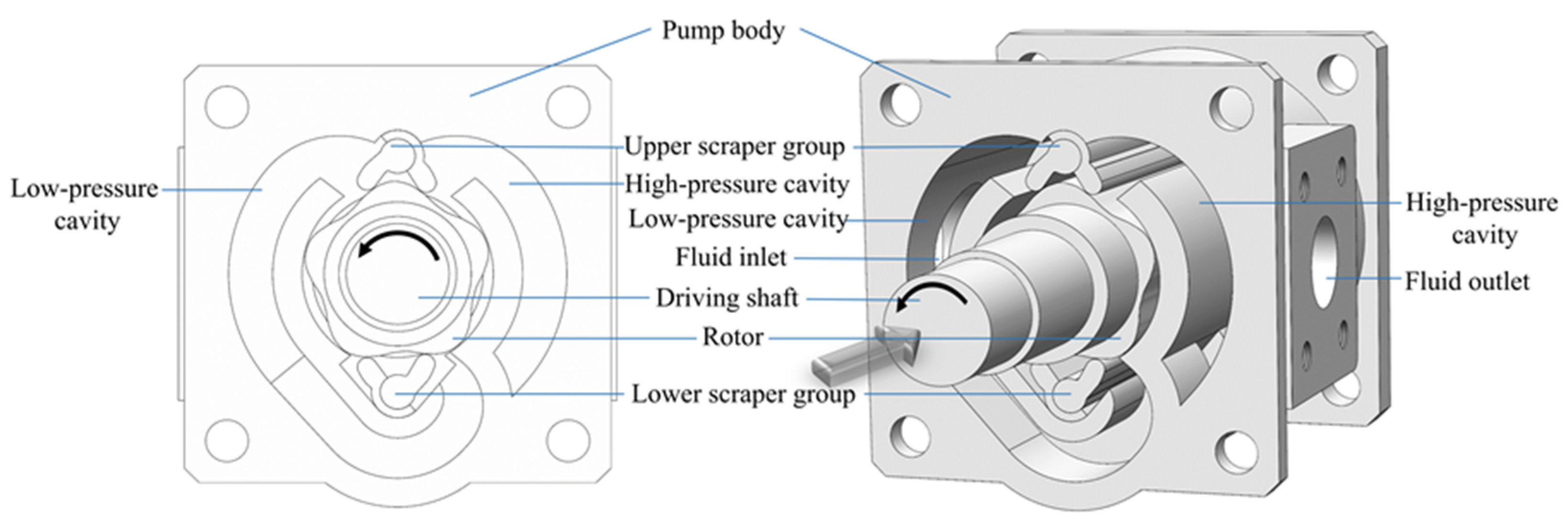They conducted computational fluid dynamics simulations of the ERSP, confirming its feasibility and advantages in enhancing fluid pressure and flow rate [18]. To further enhance the working efficiency and reduce fluid pulsation of the scraper pump, this paper proposes a double-acting five-blade rotor swing scraper pump. This pump utilizes two pairs of swinging scrapers to replace one gear in a gear pump or one rotor in a rotor pump, effectively converting the mechanical energy of the pump into fluid pressure energy. Compared to other volumetric pumps, it features a compact structure, small size, and excellent sealing. The FRSSP achieves fluid intake and discharge by making the scraper swing in response to the profile of the rotor, thereby varying the pump chamber volume and transporting the medium.

Kinematic analysis of mechanical devices is one of the indispensable steps in the research and development of mechanical devices. Mechanical structures can only realize functional requirements if they meet kinematic requirements [19,20,21,22,23]. Peng et al. proposed a novel approach for predicting the pressure and flow rate of flexible electrohydrodynamic (EHD) pumps using a Kolmogorov–Arnold Network (KAN). KAN offers exceptional accuracy and interpretability, making it a promising alternative for predictive modeling in EHD pumping applications [24]. Battarra et al. analyzed the kinematics of the vane–cam ring mechanism in a balanced vane pump, exploring the relationship between vane geometry and pump performance. They proposed a new design method to enhance the efficiency and performance of the pump [25]. Guerra et al. analyzed the kinematics of the twin lip vanes used in balanced vane pumps, deriving the trajectories, velocities, and accelerations of the vanes. They detailed how the twin lip configuration affected the kinematics of the machine and validated the feasibility of the mechanism [26]. Hou et al. proposed a kind of triplex single-function reciprocating pump driven by linear motor technology, deriving its motion laws and phase differences. They found that the pump can theoretically achieve a “constant discharge rate”, providing a theoretical basis for developing new reciprocating pumps [27]. Yuan et al. proposed a single-stage horizontal self-priming pump system composed of roots and centrifugal pumps. They conducted modeling and kinematic simulation analysis, laying the groundwork for the next steps in prototype fabrication and experimentation [28].

Through the kinematic study of the FRSSP, the scraper swing angle, angular velocity, and angular acceleration can be precisely determined. This deepens the understanding and description of the scraper pump’s motion laws and characteristics, providing a theoretical basis for the subsequent design of a kinematic pulsation-free scraper pump. Given the unique structure of the swing scraper pump, this paper proposes a kinematic analysis method for the companion trajectory of the FRSSP. The method involves deriving the rotor’s comparing theoretical from the cam profile and using this trajectory to derive the analytical equations of the scraper pump’s motion. The accuracy of this method is verified by comparing theoretical calculations with simulation results. This method is also applicable to cam mechanisms with similar swinging followers. It provides a disciplinary analysis tool for the high-precision design and optimization of rotor and scraper profiles. It offers displacement–following boundary conditions for future complex fluid–structure interaction analyses.

Section 2 describes the structural principles of the FRSSP. Section 3 establishes the rotor’s comparing theoretical equation based on the cam profile equation. Section 4 develops the kinematic model of the scraper pump based on the comparing theoretical. Section 5 conducts simulations of the FRSSP using ADAMS, comparing theoretical calculations with simulation results. A sensitivity analysis is performed on the companion trajectory kinematic analysis method for the FRSSP. Section 6 presents flow field simulation analysis and experimental validation of the FRSSP. Section 7 provides a summary of the content discussed in this study.

2. The Structural Principles of the Five-Blade Rotor Swing Scraper Pump

The structure of the FRSSP, as illustrated in Figure 1, primarily comprises the upper scraper assembly, lower scraper assembly, five-blade rotor cam, pump body, and drive shaft. The FRSSP contains four scrapers, each with an identical shape and size at the end in contact with the rotor, symmetrically distributed relative to the rotor’s center. The five-blade rotor and the swinging scraper are the core components of this pump. The swinging scraper assembly is pressed against the rotor cam by torsion springs and fluid pressure. As the five-blade rotor rotates counterclockwise, it drives the four scrapers to swing, altering the working chamber’s volume and facilitating fluid intake and discharge, achieving medium transport. The low-pressure cavity of the FRSSP has two inlets for fluid entering the working area; the corresponding high-pressure cavity has two outlets for fluid exiting the working area. Compared to a single inlet and outlet entering the working area, such a design can enhance the flow rate of the scraper pump, thereby improving its working efficiency.

When the FRSSP begins operation, external power drives the transmission shaft, causing the rotor to rotate counterclockwise. The swinging scrapers are pressed against the rotor by torsion springs, and the rotor’s rotation drives the scrapers to swing back and forth. Fluid enters the pump through the inlet. The swinging motion of the scrapers increases the volume of the low-pressure cavity and decreases the volume of the high-pressure cavity. Fluid is drawn into the low-pressure cavity, and then, as the rotor turns, it moves through the sealed chamber to the high-pressure cavity, where it is finally expelled through the outlet. Notably, when the scraper pump begins operation, the swinging scrapers adhere to the rotor under the action of torsion springs. As the volume of the high-pressure cavity decreases, the fluid pressure gradually increases. The high-pressure fluid exerts pressure on the scrapers on the high-pressure cavity side, further enhancing the contact between the scrapers and the rotor. When the rotor reverses, the fluid inlet and outlet switch accordingly. The detailed working process is illustrated in Figure 2.

3. The Companion Trajectory of the Rotor Cam

The rotor profile consists of a combination of five identical curves, which can be regarded as a superposition of a circle and a sinusoidal curve of five times the intrinsic frequency, and the parametric equation of the rotor profile is:

$$\left\{\begin{array}{l}x=(r_b+A_c\sin (5t))\cos t\\ y=(r_b+A_c\sin (5t))\sin t\\ t\in [0,2\pi ]\end{array}\right.$$

(1)

where r_b = 29.3 mm is the base circle radius of the rotor profile; A_c = 2.8 mm is the amplitude of the enclosing sine curve; and t is the parameter in the parametric equation of the rotor profile.

The parametric equations of the rotor profile are transformed into polar coordinate equations:

$$\left\{\begin{array}{l}\rho =\sqrt{x^2+y^2}=29.3+2.8\sin 5\theta \\ \theta =\arctan {\displaystyle \frac{y}{x}}=t,t\in \left[0,2\pi \right]\end{array}\right.$$

(2)

where ρ is the polar diameter; θ is the polar angle.

The scraper swing center is fixed, and the overall movement of the scraper key in determining the scraper and rotor contact with one end of the profile (can be designed as an arc) of the curvature of the center relative to the rotor rotation center of the position of the rule of change, i.e., the rotor profile of the companion trajectory, the corresponding analysis method is named as the companion trajectory kinematics analysis method.

Methods for determining the companion trajectory include vector projection and the cosine rule of triangles. This paper uses the vector projection method to derive the trajectory of the curvature circle center of the scraper’s contact end profile from the polar coordinate equation of the five-blade rotor profile. This trajectory, known as the companion trajectory, is essentially an equidistant outward offset line from the rotor profile. Assuming the polar coordinates of the rotor profile are (θ_k, ρ_k), and designing the contact portion between the scraper and the rotor as an arc with a radius R₀. Take the center of the rotor as the origin of the coordinate system, take the line between the center of the rotor and the swing center of the scraper as the Y-axis, make a straight line perpendicular to the Y-axis at the center of the rotor as the X-axis, and set up the coordinate system shown in Figure 3, and determine the companion trajectory by the profile of the five-blade rotor cam. In the figure, A is the center of the rotor; B is the swinging center of the scraper; point C indicates the contact point between the swinging scraper and the rotor; point D is the center of curvature of the contact end profile of the scraper with the rotor. TT is tangent to the rotor profile at the contact point C. Correspondingly, NN is normal at that point; ρ_k, θ_k are the polar diameters and polar angles of the rotor profile, respectively; r_k, ψ_k are the polar diameters and polar angles of the companion trajectories, respectively; μ_k is the angle between the polar diameter ρ_k of the rotor profile at the contact point C and its tangent line TT at point C; λ_k is the angle between the tangent TT of the rotor profile at point C and the X-axis in the positive direction; η_k is the angle between the normal NN of the rotor profile at point C and the positive X-axis.

From Figure 3, it can be observed that: $\overrightarrow{AD}=\overrightarrow{AC}+\overrightarrow{CD}$. The projections onto the X-axis and Y-axis are:

$$\left\{\begin{array}{l}{x}_k={\rho }_k\cos {\theta }_k+R_0\cos {\eta }_k\\ y_k={\rho }_k\sin {\theta }_k+R_0\sin {\eta }_k\end{array}\right.$$

(3)

Based on the vector relationship, the polar radius r_k and polar angle ψ_k of the companion trajectory of the five-blade rotor cam can be derived as follows:

$$\left\{\begin{array}{l}{r}_k=\sqrt{x_k^2+y_k^2}=\sqrt{{\left({\rho }_k\cos {\theta }_k+R_0\cos {\eta }_k\right)}^2+{\left({\rho }_k\sin {\theta }_k+R_0\sin {\eta }_k\right)}^2}\\ {\psi }_k=\arctan {\displaystyle \frac{y_k}{x_k}}=\arctan {\displaystyle \frac{\left({\rho }_k\sin {\theta }_k+R_0\sin {\eta }_k\right)}{\left({\rho }_k\cos {\theta }_k+R_0\cos {\eta }_k\right)}}\end{array}\right.$$

(4)

After a straightforward derivation, the expressions for μ_k, λ_k, and η_k are, respectively:

$${\mu }_k=\arctan {\displaystyle \frac{{\rho }_k}{{{\rho }^{\prime }}_k}}$$

(5)

$${\lambda }_k={\theta }_k+{\mu }_k$$

(6)

$${\eta }_k={\lambda }_k-90={\theta }_k+{\mu }_k-90$$

(7)

where ${\rho }_k^{’}={\displaystyle \frac{\mathrm{d}{\rho }_k}{\mathrm{d}\theta }}$.

4. Kinematic Modeling Based on the Companion Trajectory

In order to describe more clearly the process of deducing the scraper pump kinematics from the companion trajectory of the five-blade rotor cam, the rotor profiles in Figure 3 were removed. The positional relationship between the companion trajectory and the center of curvature D of the profiles at the contact end of the scraper with the rotor was used to form Figure 4, which was used to determine the parameters. In the figure, T₁T₁ is tangent to the companion trajectory at point D, and NN is normal at point D; r₀ is the radius of the base circle of the companion trajectory; D₀ is the intersection of the arc drawn with a radius of the length of BD and the base circle; β₀ is the initial position angle of the scraper; β_k is the swing angle of the scraper; point P represents a point on the companion trajectory and base circle. B_p is the position of the center of the swing of the scraper at the moment of the initial position angle determined by the inverse method; point E is the intersection of the normal NN with the Y-axis; a perpendicular line is drawn from point E to BD, intersecting the extension of BD at point F; V_D represents the velocity direction at point D.

4.1. Determine the Swing Angle and Pressure Angle of the Scraper

Figure 4 shows the relationship between the five-blade rotor cam companion trajectory and the swinging scraper motion pattern. In order to show more clearly the derivation process between the rotor companion trajectory and each motion characteristic of the scraper, Figure 4 is decomposed into Figure 5a,b.

As shown in Figure 5a, to determine the oscillation angle of the scraper when the curvature center of the scraper profile at the contact end with the rotor is at point D, it is necessary to know the lowest position of the scraper. The reverse method is used to ascertain the scraper’s lowest position. The rotor cam is known to rotate counterclockwise. Draw a circle with A as the center and the length of AB as the radius to represent the circle of the trajectory of the pump body. Take P point as the center of the circle, take the length of BD as the radius, draw a circle, and intersect with the trajectory circle of the pump body at two points. According to the reverse method, B_p is the center of the scraper’s swing when it is in the lowest position. Connect AB_p and B_pP, then ∠AB_pP is the initial position angle of the scraper. β_k = ∠ABD − ∠AB_pP, which is the swing angle of the scraper. Take B as the center of the circle, BD as the radius to draw a circular arc, and intersect with the base circle at point D₀; connect BD₀ and AD₀, and get △ABD₀ and △AB_pP are congruent, so β₀ = ∠AB_pP, and thus β_k = ∠ABD − β₀.

Based on trigonometric relationships and the law of cosines, the specific expression for β_k can be derived as follows:

$${\beta }_k=\arccos {\displaystyle \frac{h^2+l^2-r_k^2}{2hl}}-{\beta }_0$$

(8)

where h is the distance from the rotor rotating center to the swinging center of the scraper; l is the length of the scraper; β₀ is the initial position angle of the scraper and its specific expression is:

$${\beta }_0=\arccos {\displaystyle \frac{h^2+l^2-r_0^2}{2hl}}$$

(9)

As shown in Figure 5b, the acute angle α_k formed by the velocity at point D on the scraper and the normal NN at point D on the companion trajectory of the rotor cam is the pressure angle of the scraper, and the magnitude of the pressure angle can be deduced from the above figure. From the figure, BD is perpendicular to the direction of velocity at point D; the normal NN at point D is perpendicular to the tangent T₁T₁, so the magnitude of the acute angle subtended by the tangent and BD is equal to the angle of pressure, which can be derived directly from the angular relationship in the figure. So, the specific expression for the scraper pressure angle is:

$${\alpha }_k=\tau -90-\left({\psi }_k-{\eta }_k\right)$$

(10)

where τ is the angle between the scraper BD and the pole diameter AD, and its expression is:

$$\tau =\arccos {\displaystyle \frac{l^2+r_k^2-h^2}{2l{r}_k}}$$

(11)

4.2. Determine the Rotation Angle of the Rotor Cam

Take the starting position of the companion trajectory of the rotor cam as a reference and apply the reverse method to find the rotation angle of the rotor cam. As shown in Figure 6, D₁ is the position of the start point of the companion trajectory at θ_k = 0, r₁ is the polar diameter at that point, and ψ₁ is the polar angle at that point. AB₁ is the starting position of the pump body when the scraper is in position D₁. The rotor cam rotates counterclockwise, and when a certain instantaneous scraper is located at the BD position, it is known by the inverse method that the pump body rotates clockwise from AB₁ to the AB position at the angle turned is the rotation angle φ_k of the cam.

Based on trigonometric relationships and the cosine theorem, the specific expression for φ_k can be derived.

$${\phi }_k=2\pi -\left[\left({\psi }_k+\arccos {\displaystyle \frac{h^2+r_k^2-l^2}{2h{r}_k}}\right)-\left({\psi }_1+\arccos {\displaystyle \frac{h^2+r_1^2-l^2}{2h{r}_1}}\right)\right]$$

(12)

4.3. Determine the Angular Velocity of the Scraper

Let the angular velocity of the scraper be Ω_k when the rotor rotation angle is φ_k. Point E is the intersection of the normal NN and BA, as shown in Figure 5b. From the three-center theorem, point E is the instantaneous center of the relative velocity of the rotor and the scraper, so the rotor and the scraper have the same linear velocity at point E; thus:

$${\Omega }_k\cdot BE=\omega \cdot AE\Rightarrow {\displaystyle \frac{{\Omega }_k}{\omega }}={\displaystyle \frac{AE}{BE}}={\displaystyle \frac{h-BE}{BE}}$$

(13)

where ω is the angular velocity of the rotor.

Make the plumbline EF of BD at point E. Then ∠DEF = α_k. From the right triangle DEF, the following can be obtained:

$$\tan {\alpha }_k={\displaystyle \frac{DF}{EF}}={\displaystyle \frac{BE\cos \left({\beta }_0+{\beta }_k\right)-l}{BE\sin \left({\beta }_0+{\beta }_k\right)}}\Rightarrow BE={\displaystyle \frac{l}{\cos \left({\beta }_0+{\beta }_k\right)-\tan {\alpha }_k\sin \left({\beta }_0+{\beta }_k\right)}}$$

(14)

By combining Equations (13) and (14), the angular velocity of the scraper can be determined:

$${\Omega }_k=\left({\displaystyle \frac{h}{BE}}-1\right)\omega =\left\{{\displaystyle \frac{h\left[\cos \left({\beta }_0+{\beta }_k\right)-\tan {\alpha }_k\sin \left({\beta }_0+{\beta }_k\right)\right]}{l}}-1\right\}\omega$$

(15)

4.4. Determine the Angular Acceleration of the Scraper

The angular velocity of the scraper has been derived from Section 4.3, but since the independent variable of the angular velocity in this text is not time t, directly differentiating with respect to time t will not yield the angular acceleration. The differentiation equation needs to be transformed to determine the angular acceleration of the scraper:

$$\epsilon ={\displaystyle \frac{d\Omega }{dt}}={\displaystyle \frac{d\Omega }{d\phi }}\cdot {\displaystyle \frac{d\phi }{dt}}=\omega \cdot {\displaystyle \frac{d\Omega }{d\phi }}$$

(16)

where ε is the angular acceleration of the scraper, Ω is the angular velocity of the scraper, φ is the rotation angle of the rotor.

From Equation (16), it can be seen that to require the angular acceleration of the scraper, it is necessary to first find the derivative of the angular velocity of the scraper with respect to the rotor rotation angle. The angular velocity of the scraper and the rotor rotation angle are derived from the companion trajectory of the rotor cam. Numerical analysis can be used to fit the calculated scraper angular velocity data with the rotor rotation angle data to obtain an approximate relationship curve. Different fitting methods to obtain the curve results are different; using the appropriate method for fitting the curve can be a more realistic response to the relationship between the scraper angular velocity and the rotor rotation angle, which is extremely important. This paper uses MATLABR2021b software to calculate the scraper angular velocity and the rotor rotation angle, using the software’s curve fitting toolbox, the choice of sum of sine method to fit the relationship between Ω and φ curve. The fitting formula is:

$$\begin{array}{l}\Omega =a_1\cdot \sin \left(b_1\cdot \phi +c_1\right)+a_2\cdot \sin \left(b_2\cdot \phi +c_2\right)+a_3\cdot \sin \left(b_3\cdot \phi +c_3\right)+a_4\cdot \sin \left(b_4\cdot \phi +c_4\right)+\\ a_5\cdot \sin \left(b_5\cdot \phi +c_5\right)+a_6\cdot \sin \left(b_6\cdot \phi +c_6\right)+a_7\cdot \sin \left(b_7\cdot \phi +c_7\right)+a_8\cdot \sin \left(b_8\cdot \phi +c_8\right)\end{array}$$

(17)

where a₁, b₁, c₁, a₂, b₂, c₂, …are the coefficients derived from the software MatlabR2021b, and the specific magnitudes are shown in

Table 1. Numerical magnitude of coefficients.

	Coefficient	ai	bi	ci
Subscript Value i
1		259.6	3.839	1.793
2		128	7.518	0.5978
3		109.7	1.145	6.649
4		55.07	12.32	−7.058
5		14.81	14.04	9.606
6		32.73	17.9	6.701
7		18.01	23.31	−3.821
8		6.051	27.52	−7.985

below.

The derivative of the scraper angular velocity with respect to the rotor angle dΩ/dφ:

$$\begin{array}{l}{\Omega }^{\prime }\left(\phi \right)=a_1\cdot b_1\cdot \cos \left(b_1\cdot \phi +c_1\right)+a_2\cdot b_2\cdot \cos \left(b_2\cdot \phi +c_2\right)+a_3\cdot b_3\cdot \cos \left(b_3\cdot \phi +c_3\right)+\\ a_4\cdot b_4\cdot \cos \left(b_4\cdot \phi +c_4\right)+a_5\cdot b_5\cdot \cos \left(b_5\cdot \phi +c_5\right)+a_6\cdot b_6\cdot \cos \left(b_6\cdot \phi +c_6\right)+\\ a_7\cdot b_7\cdot \cos \left(b_7\cdot \phi +c_7\right)+a_8\cdot b_8\cdot \cos \left(b_8\cdot \phi +c_8\right)\end{array}$$

(18)

By combining Equations (16) and (18), the angular acceleration of the scraper can be determined.

5. Kinematic Verification of a Five-Blade Rotor Swing Scraper Pump Based on ADAMS

ADAMS 2020 is the definitive mechanical kinematics and dynamics simulation and analysis software for predicting the performance of mechanical systems, range of motion, crash monitoring, peak loads, and calculating input loads for finite elements. In the following, MATLAB programming calculates the kinematic characteristics of the FRSSP. Then, ADAMS performs a kinematic simulation of the FRSSP. Finally, the obtained theoretical calculations are compared with the simulation results to check the accuracy of the above theoretical analysis.

5.1. Kinematic Simulation of the FRSSP

The basic structural parameters of the FRSSP are shown in

Table 2. Basic parameters of the five-blade rotor swing scraper pump.

Parameter	Value
Length of scraper l	13.47 mm
The radius of curvature of the scraper R0	3.34 mm
Distance from rotor slewing center to scraper swing center h	41 mm
The radius of the base circle of the rotor companion trajectory r0	29.84 mm
The angular velocity of the rotor cam ω	230.38 rad/s

below. The swing scraper, five-blade rotor cam, and pump body of the scraper pump are all made of aluminum alloy. The material properties of aluminum alloy are listed in

Table 3. Material properties of Al alloy.

Material	Modulus of Elasticity (MPa)	Poisson Ratio	Yield Strength (MPa)	Tensile Strength (MPa)	Density (kg/m3)
Aluminum alloy	7.1 × 104	0.33	240	290	2770

.

Based on the conditions mentioned above, the kinematic characteristics of the FRSSP can be calculated in MATLAB. Subsequently, according to real-world conditions, the model of the FRSSP is configured in ADAMS, setting up contacts, connections, and drives. Figure 7 illustrates the ADAMS simulation flowchart.

During the kinematic simulation analysis of the FRSSP in ADAMS, as shown in Figure 7, the first step is to convert the 3D model of the pump into a compatible format and import it into ADAMS. To ensure that the simulation results closely approximate reality and accurately reflect the actual kinematic characteristics of the pump, the materials of all components are defined as aluminum alloy. A fixed joint is created for the pump body to keep it stationary throughout the simulation. Revolute joints are applied to the rotor and swing scraper, allowing the scraper and rotor to rotate according to the actual motion directions. A drive is applied to the rotor, setting it to rotate counterclockwise at a speed of 2200 r/min. Gravity is applied to the entire system, and contact interactions are defined between the rotor and the swing scraper. A spring force is added to the swing scraper to ensure it maintains continuous contact with the rotor surface, with both contact and spring settings kept at the software’s default values.

The initial state of the simulation is set with the five-blade rotor in a left–right symmetrical position. To verify the accuracy of the calculated results, the first four cycles of the pump’s operation are analyzed in detail.

Figure 8 shows the theoretical and simulation curves of the swing angle of the scraper in four cycles, from which it can be seen that the scraper pump runs for one cycle, the rotor rotates one circle, and the swing scraper swings up and down five times. The theoretical calculation of the maximum swing angle is 28.3427°, and the simulation simulates a maximum swing angle of 28.8671°, with an error of 1.85%. The kinematic study method proposed in this paper can accurately solve the swing angle of the scraper of the FRSSP.

Figure 9 shows the theoretical and simulation plots of the rotor cam rotation angle over four cycles. In the text, the counterclockwise rotation of the rotor is defined as positive. As shown in the figure, the rotor cam rotates one complete turn counterclockwise for each operational cycle of the scraper pump. The cam rotation angle from theoretical calculations matches the simulation results, with the two curves fitting closely. The kinematic study method proposed in this paper can accurately solve the cam rotation angle of the FRSSP.

Figure 10 shows the theoretical and simulated curves of the scraper angular velocity over four cycles. As can be seen from the figure, the angular velocity curve of the scraper obtained from the simulation has a significant fluctuation at 0.001 s, which is caused by the fact that the model of the scraper pump used in this paper leaves a small gap between the cam rotor and the swing scraper, which results in the collision of the rotor and the scraper when the scraper pump starts to operate. The theoretical calculation of the maximum angular velocity of the swinging scraper in the return process is 218.449 rad/s, and the maximum angular velocity in the push process is 404.497 rad/s. The maximum angular velocity of the swinging scraper in the return process simulated by ADAMS is 237.863 rad/s, with an error of 3.11%; the maximum angular velocity in the push process is 435.254 rad/s, the error is 4.93%. The angular velocity change trend of the theoretical calculation and simulation curves is basically the same. It can be seen that the kinematic research method proposed in this paper can accurately solve the scraper angular velocity of the FRSSP.

Figure 11 shows the theoretical and simulated curves of the scraper angular acceleration over four cycles. The figure shows that the angular acceleration curve of the scraper obtained from the simulation will have a significant fluctuation at the beginning, which is caused by the collision between the rotor and the scraper. The theoretical calculation of the maximum angular acceleration of the swing scraper in the return process is 3.52 × 10⁵ rad/s²; the maximum angular acceleration in the push process is 8.20 × 10⁵ rad/s². ADAMS simulation simulates that the maximum angular acceleration of the swing scraper in the return process is 3.81 × 10⁵ rad/s², with an error of 2.47%; the maximum angular acceleration in the push process is 8.33 × 10⁵ rad/s², with an error of 1.11%. The theoretical calculation curve of scraper angular acceleration has the same trend as the simulation curve. It can be seen that the kinematic research method proposed in this paper can accurately solve the scraper angular acceleration of the FRSSP.

Figure 12 shows the resultant curve calculated by the theoretical formula for the pressure angle of the scraper. The minimum pressure angle of the scraper is 3.32°, and the maximum pressure angle is 61.86°. According to experience, it can be known that the permissible pressure angle of the scraper follower for the push stroke [α₁] = 30°, and the permissible pressure angle for the return stroke [α₂] = 70°~80°, so that the FRSSP can operate normally.

5.2. Sensitivity Analysis of the Kinematic Calculation Method for the FRSSP

In Section 5.1, the kinematic characteristics of the FRSSP under specific dimensions were calculated using the kinematic analysis method proposed in this study, and the results were validated through ADAMS simulations. The findings indicate that the kinematic analysis method for the FRSSP derived in Section 4 is relatively accurate. To verify the robustness of this method, a comparative analysis was conducted by altering the geometric parameters of key components of the FRSSP. The specific parameters are listed in the

Table 4. Parameters of the four scraper pump sets.

Parameters	Values
l (mm)	13	12.5	13.8	13.47
R0 (mm)	3	3.5	3.7	3.34
r0 (mm)	29.5	30	30.2	29.84
ω (rad/s)	174.53	157.08	188.5	230.38
rb (mm)	29.3	29.3	29.3	30.1
Ac (mm)	2.8	2.8	2.8	3.1
Parameter sets	1	2	3	4

.

Using the kinematic analysis method for the FRSSP proposed in this study, the parameters from each set in Table 4 were substituted into the analysis to obtain the theoretical calculation results for each pump. Based on Table 4, four three-dimensional models of scraper pumps with different parameters were established using modeling software for simulation analysis, yielding simulation results. A comparison was conducted between the theoretical and simulation results of the FRSSP from three perspectives: the swing angle of the scraper, the angular velocity of the scraper, and the angular acceleration of the scraper. The results obtained from theoretical calculations and simulation analyses are shown in the

Table 5. Theoretical calculation results and simulation results of scraper pumps with different parameters.

	Parameter Sets	1		2		3		4
Result Parameters		Theoretical	Simulation	Theoretical	Simulation	Theoretical	Simulation	Theoretical	Simulation
Scraper swing angle (dec)		31.36	31.98	32.34	32.97	26.56	27.11	30	30.64
Return stroke angular velocity (rad/s)		174.02	179.99	162.86	163.55	173.26	185.57	235.90	240.36
Push stroke angular velocity (rad/s)		383.43	398.87	350.38	362.93	288.74	307.95	409.53	430.42
Return stroke angular acceleration (rad/s2)		3.16 × 105	3.25 × 105	2.57 × 105	2.75 × 105	1.77 × 105	1.84 × 105	3.32 × 105	3.77 × 105
Push stroke angular acceleration (rad/s2)		6.26 × 105	6.39 × 105	5.26 × 105	5.52 × 105	4.62 × 105	4.71 × 105	8.27 × 105	8.53 × 105

.

Based on the data in Table 5, the errors between the theoretical calculations and simulation results for each scraper pump can be computed. Combining the error results obtained in Section 5.1, the errors for each result are presented, as shown in

Table 6. Errors between the theoretical calculation results and simulation results of the scraper pump.

	Parameter Sets	1	2	3	4	5
Result Parameters
Scraper swing angle		1.98%	1.95%	2.07%	2.13%	1.85%
Return stroke angular velocity		1.07%	0.13%	2.66%	0.69%	3.11%
Push stroke angular velocity		2.77%	2.45%	4.16%	3.24%	4.93%
Return stroke angular acceleration		0.96%	2.30%	1.10%	3.88%	2.47%
Push stroke angular acceleration		1.38%	3.32%	1.41%	2.24%	1.11%

.

In the table, parameter set 5 represents the error results obtained in Section 5.1. Excluding errors caused during the modeling process, the data in Table 6 show that the errors between the results obtained using the companion trajectory kinematic analysis method and the simulation results for the five different parameter sets of scraper pumps are all within 5%. This demonstrates the strong robustness of the companion trajectory kinematic analysis method proposed in this study.

6. FRSSP Flow Field Simulation and Experiments

This section conducts a flow field analysis of the FRSSP to validate its feasibility and explore its flow field characteristics. Advanced CFD software is utilized for fluid simulation of the FRSSP. The flow field characteristics of the scraper pump are simulated at a rotor speed of 1500 r/min, followed by experiments to compare and discuss the experimental and simulation data.

6.1. FRSSP Flow Field Simulation Analysis

In this study, XFlow software is utilized for flow field simulation of the FRSSP. XFlow 2022 adopts a numerical solution scheme based on the Lattice Boltzmann Method (LBM), which is well-suited for simulating complex flow problems. Moreover, XFlow efficiently leverages multi-core CPUs and GPUs, significantly enhancing computation speed for large-scale simulations. Additionally, XFlow’s automatic mesh generation and adaptive mesh refinement features dynamically optimize mesh resolution according to flow field variations, avoiding the challenges of mesh division in complex geometries and flow conditions often encountered with traditional CFD software. This characteristic eliminates the need for mesh independence testing, thereby improving simulation efficiency. To simulate the boundary layer, XFlow uses a unified nonequilibrium wall function. This wall model is universally applicable, eliminating the need to select between different algorithms, thus improving simulation efficiency.

Before conducting the fluid simulation for the scraper pump, the simulation parameters must be configured. The 3D model of the FRSSP is imported into XFlow software. The rotor speed is set to 1500 r/min, and the angular velocity of the scrapers obtained from ADAMS kinematic simulations is imported into XFlow. Hydraulic oil is selected as the fluid medium, with a density of 865 kg/m³ and a dynamic viscosity of 0.01 Pa·s. The outlet load pressure is set to 2 MPa, and the inlet load pressure to 0.1 MPa. The simulation time is 0.04 s, with a time step of 2 × 10⁻⁶ s. Using these parameters, a single-phase fluid simulation of the scraper pump is carried out.

When the rotor completes one full rotation, the upper and lower oil chambers of the scraper pump each perform five cycles of oil intake and discharge. Specifically, for every 72° of rotor rotation, the scraper pump conducts two cycles of oil intake and discharge. To provide a clearer visualization of the pressure field, planes were established within three flow channels to better observe the pressure variations across each channel. Key positions of the scraper pump were selected to analyze the pressure field distribution within the pump chamber.

Figure 13 illustrates the pressure field distribution inside the pump chamber of the FRSSP at a rotor speed of 1500 r/min. Panels (a) to (d) depict the process of the rotor completing a 72° rotation, during which the upper and lower oil chambers of the scraper pump each perform one cycle of oil intake and discharge. The fluid enters through the inlet, passes through the low-pressure channel into the sealed chamber, where the pressure rises, and then flows through the high-pressure channel and exits at the fluid outlet. During this process, the inlet pressure remains around 0.1 MPa, the pump chamber pressure connected to the outlet ranges between 1.6 and 2 MPa, and the outlet pressure stabilizes at approximately 2.1 MPa.

Figure 14 illustrates the distribution of the velocity vectors within the pump chamber of the FRSSP at a rotor speed of 1500 r/min. Panels (a) to (d) show the process of the rotor completing a 72° rotation. The simulation results reveal that the velocity variation is minimal on the front and rear sides of the scraper pump, with significant changes in velocity concentrated in the middle section of the pump. To better visualize the velocity vector distribution, the images on the right side of the figure display the velocity variations at the middle cross-section. From the figure, it can be observed that the fluid velocity in the low-pressure channel is relatively low, ranging from approximately 0.5 to 1.5 m/s. As the fluid enters the sealed chamber, the velocity increases due to the rise in pressure. Under the influence of gravity and the high-pressure channel’s location, when the fluid enters the upper high-pressure channel, it must overcome gravity, resulting in a lower velocity. The velocity reaches its maximum as the fluid enters the lower high-pressure channel, with a peak speed of 24.3 m/s.

The simulation results show that at a rotor speed of 1500 r/min, the instantaneous maximum flow rate at the outlet of the scraper pump is 6.74 kg/s, with an average flow rate of 4.75 kg/s. To later validate the accuracy of the simulation through experimentation, multiple flow field simulations were conducted at different rotor speeds. At a rotor speed of 1200 r/min, the scraper pump’s outlet exhibits an instantaneous maximum flow rate of 4.55 kg/s and an average flow rate of 3.94 kg/s. At a rotor speed of 1667 r/min, the instantaneous maximum flow rate is 7.83 kg/s, with an average flow rate of 5.28 kg/s.

6.2. Experiment

Based on theoretical analysis, model construction, kinematic analysis, and flow field analysis, a prototype of the scraper pump was manufactured, as shown in Figure 15d,e. To validate the feasibility of the scraper pump and the accuracy of the simulation results, experiments were conducted. The experiment involved measuring the outlet flow rate of the scraper pump at different operating speeds using the YST400W hydraulic (The manufacturer of the YST400W hydraulic test rig is Jinan Highland Hydraulic Pump Co., Ltd., located in Jinan, China.) test rig. The ultimate aim was to validate the feasibility of the scraper pump’s working principle and the accuracy of the simulation results.

The YST400W hydraulic test rig is a specialized platform for testing and inspecting hydraulic pumps and motors. It is designed for comprehensive testing of hydraulic pumps and motors and consists primarily of a motor power unit, a main fuel tank valve console, and an operation console. The experimental setups for each part are shown in Figure 15a–c.

The rotor shaft of the experimental prototype is connected to the motor, which is set to a constant rotational speed. After the pump reaches a stable operating state, the oil supply system is activated. The flow rate is displayed on the control panel, and the value is recorded once it stabilizes. To facilitate comparison with the flow field simulation results, the motor speeds are set to 1200 r/min, 1500 r/min, and 1667 r/min, respectively. To enhance the accuracy of the experimental data, three sets of experiments are conducted for each speed, and the average of these sets is used as the final data. The structure of the experimental prototype is largely consistent with the three-dimensional model used in the flow field simulation; however, due to engineering design issues, there are minor discrepancies that may affect the experimental results. As a result, some deviation is expected between the simulation data and the experimental data. Nevertheless, as long as the error between the two remains within 5%, they can be considered mutually corroborative. The experimental results are presented in

Table 7. Comparison of Experimental and Simulation Results.

Rotor Speed	Outlet Flow Rate		Error
	Simulation Results	Experimental Results
1200 r/min	3.94 kg/s	3.81 kg/s	3.30%
1500 r/min	4.75 kg/s	4.58 kg/s	3.58%
1667 r/min	5.28 kg/s	5.07 kg/s	3.98%

and compared with the flow field simulation results.

The results indicate that the flow field simulation results of the scraper pump show an error within 5% of the experimental results, validating both the feasibility of the scraper pump’s structural principles and the accuracy of the flow field simulation. Since the scraper angular velocity used in the flow field simulation was derived from the ADAMS simulation, this experiment indirectly confirms the accuracy of the ADAMS kinematic simulation. In turn, this serves as indirect evidence for the accuracy of the companion trajectory kinematic analysis method proposed in this study.

7. Conclusions

As an innovative fluid dynamic device, the five-blade rotor swing scraper pump utilizes a rotating cam–swing scraper mechanism to achieve fluid intake and discharge. Its compact structure, self-sealing properties, and high working efficiency make it suitable for a wide range of applications. Using a method based on the study of the companion trajectory kinematics of the five-blade rotor swing scraper pump, the kinematic parameters of the pump were calculated. Subsequently, the pump underwent kinematic simulations and flow field simulations, which were further validated through experiments. The main conclusions of this study are as follows.

(1)

A comparison between the theoretical results obtained through the companion trajectory kinematics analysis method and the ADAMS simulation results reveals that the error in the scraper swing angle is 1.85%; the rotation angle of the rotor cam is identical; the maximum error in the scraper angular velocity is 4.93%; and the maximum error in the scraper angular acceleration is 2.47%. The results obtained from the theoretical calculation and simulation are within 5% error, which verifies the accuracy of the kinematic research method, and the method can serve as a boundary condition for the optimal design of the rotor profile and scraper profile, providing a theoretical basis for the subsequent design of kinematic pulsation-free scraper pump.

(2)

A sensitivity analysis of the companion trajectory kinematics analysis method was conducted by varying the dimensional parameters of key components of the FRSSP. Five different scraper pump models with varying parameters were obtained. A comparison between the theoretical calculations and simulation results under the same parameters showed that the error in all cases was within 5%, demonstrating that the proposed companion trajectory kinematics analysis method exhibits strong robustness.

(3)

Flow field simulation analysis and experiments were conducted on the scraper pump, and the flow rates at the pump outlet under different rotational speeds were obtained. A comparison of the simulation and experimental results revealed that the error between the two was within 5%, allowing them to corroborate each other since the scraper angular velocity used in the flow field simulation was derived from the ADAMS simulation, which indirectly verified the accuracy of the ADAMS kinematic simulation results and, in turn, confirmed the accuracy of the companion trajectory kinematics analysis method proposed in this study.