Development of a Virtual Telehandler Model Using a Bond Graph

Abstract

Recent technological advancements and evolving regulatory frameworks are catalysing the integration of renewable energy sources in construction equipment, with the objective of significantly reducing greenhouse gas emissions. The electrification of non-road mobile machinery (NRMM), particularly self-propelled Rough-Terrain Variable Reach Trucks (RTVRT) equipped with telescopic booms, presents notable stability challenges. The transition from diesel to electric propulsion systems alters, among other factors, the centre of gravity and the inertial matrix, necessitating precise load capacity determinations through detailed load charts to ensure operational safety. This paper introduces a virtual model constructed through multiphysics modelling utilising the bond graph methodology, incorporating both scalar and vector bonds to facilitate detailed interconnections between mechanical and hydraulic domains. The model encompasses critical components, including the chassis, rear axle, telescopic boom, attachment fork, and wheels, each requiring a comprehensive three-dimensional treatment to accurately resolve spatial dynamics. An illustrative case study, supported by empirical data, demonstrates the model’s capabilities, particularly in calculating ground wheel reaction forces and analysing the hydraulic self-levelling behaviour of the attachment fork. Notably, discrepancies within a 10% range are deemed acceptable, reflecting the inherent variability of field operating conditions. Experimental analyses validate the BG-3D simulation model of the telehandler implemented in 20-SIM establishing it as an effective tool for estimating stability limits with satisfactory precision and for predicting dynamic behaviour across diverse operating conditions. Additionally, the paper discusses prospective enhancements to the model, such as the integration of the virtual vehicle model with a variable inclination platform in future research phases, aimed at evaluating both longitudinal and lateral stability in accordance with ISO 22915 standards, promoting operator safety.

1. Introduction

The development of non-road mobile machinery (NRMM), particularly self-propelled Rough-Terrain Variable Reach Trucks (RTVRT) used for handling loads equipped with a telescopic lifting means (pivoted boom) as Figure 1, on which a load handling device (e.g., carriage and fork arms) is influenced by various factors ranging from customer needs to fuel prices and regulations. The original equipment manufacturers industry (OEMs) is rapidly shifting towards electric solutions due to stricter emissions regulations and high fuel costs. The use of internal combustion engines presents challenges in indoor applications and urban zones due to exhaust gases. The electrification and hybridisation of these vehicles are seen as promising ways to reduce energy consumption and emissions.

Compact hydraulic telehandlers offer a compelling solution, combining the lifting capabilities of traditional telehandlers with the compact size and manoeuvrability needed for urban environments. With their ability to navigate narrow access points, reach high elevations, and handle various materials, compact telehandlers are becoming indispensable for construction, agriculture, warehousing, and maintenance tasks.

One of the key factors contributing to their versatility is their manoeuvrability, which allows for easy operation and versatility. However, it makes room for unsafe usage and is one of the most significant challenges.

Vehicle stability in all operational conditions is a crucial challenge because it directly impacts the operator’s safety. Because of this, it is exciting to quantify the degree of stability of the machine during its movement and how close or how far the machine is from losing stability, to know, for example, when the arm raises and extends its robustness against external disturbances when moving on uneven terrain or climbing a ramp.

The aspect of stability is of utmost importance, as has been indicated, highlighting the significance of this factor even in light of the existing international standards that address the safety requirements of telehandlers in terms of stability. Priora G., 2019, summarises the applicable regulations in his thesis [1]. The safety of machines in Europe is imposed by the Machinery Regulation (UE) 2023/1230 [2] and is deployed in multiple standards, among which EN/TS 1459-8:2018 [3], EN 15000:2008 [4], ISO 22915-14 2010 [5], and ISO 10896-1:2020 [6]. One of the main limitations of these standards is that they need to adequately consider dynamic loads, such as inertia, which can jeopardise the machine’s stability. Dynamic loads, caused by movements of the telescopic boom or sudden changes in load distribution, introduce additional forces and moments that can affect the stability.

Real data of the Health & Safety Executive, HSE (UK) [7], demonstrate that the primary cause of instability and overturning in telescopic handlers is lateral, followed by longitudinal, identifying the risk factors associated with overturning accidents as says Figure 2.

Longitudinal stability refers to the stability along the machine’s centreline, precisely its tendency to tip forward or backwards. As the load handled increases or the boom extends, the longitudinal load moment increases, causing the rear axle to become lighter.

Lateral stability refers to the stability at right angles to the machine’s centreline, which is precisely its tendency to lean sideways. When a load is lifted, the centre of gravity of the entire machine rises. This behaviour is not an issue if the machine is level; however, if the machine is on a slope, the centre of gravity will shift towards the tipping line as the load is lifted, causing a risk of tipping. Any attempt to turn will introduce additional centrifugal force that can result in a rollover. The summary of causes depending on the stability type can be seen in

Table 1. (a) Longitudinal stability compromises; (b) lateral stability compromises.

Longitudinal Stability Compromised by the Following:			Lateral Stability Compromised by the Following:
Action		Cause	Action		Cause
Load raising/lowering movement	Boom lifting/Extension	Gravitational force	Load transportation	Vehicle braking	Inertial force
Load lowering	Sudden boom braking	Inertial force	Travelling on uneven surfaces	Potholes, bumps, ramps, slopes	Gravitational/inertial force
Load transportation	Vehicle braking	Inertial force	Specific eccentric loads		Gravitational/inertial force
Travelling on uneven surfaces	Potholes, bumps, ramps, slopes	Gravitational/inertial force	Suspended load		Gravitational/inertial force
Suspended load		Gravitational/inertial force	Wind		External force
(a)			(b)

.

Considering the challenges above, it is essential to develop a modular, customizable, and structured virtual model of the machine based on object-oriented physical system modelling.

This article represents the first step in a broader project to study the global stability of telehandler machines. In this initial work, we focus exclusively on longitudinal stability, analysing the lifting and lowering motion of the boom fork assembly and the fork’s self-levelling mechanism, which are key functionalities for the machine’s safe performance.

The behaviour of the mobile machinery shown in Figure 3 provides a general interconnection overview, showing various stages that can be followed. The followed pathway is highlighted with a thicker line.

The main contributions of this paper are as follows:

A virtual prototype model of the compact hydraulic telehandler was developed exclusively using a graphical modelling methodology known as a Bond Graph. This methodology is particularly advantageous for multidisciplinary modelling, as it facilitates the seamless integration of both mechanical and hydraulic systems through a consistent, standardised, and unified notation. Additionally, this model is open-ended, allowing for easy modifications and extensions.

A comprehensive dynamic analysis was conducted using this virtual model to identify various scenarios that threaten the longitudinal stability of the machine, focusing mainly on one of its primary functionalities: lifting and lowering loads. The efficacy of this strategy was validated through a series of targeted tests conducted on an appropriately instrumented prototype machine.

An innovative methodology for simulating hydraulic cylinders is proposed, leveraging 1D-BG and 3D-BG (scalar and vectoral Bond Graphs). This approach enables a detailed interconnection between the mechanical and hydraulic domains, providing a highly accurate representation of cylinder dynamics. Notably, our literature review indicates that this specific application of 3D-BG and 1D-BG for simulating a hydraulic circuit has not been previously addressed, underscoring the novelty and potential impact of our contribution.

The paper is organised as follows:

The Section 2, titled “Multiphysics Modelling”, provides an overview of the mathematical formulation, software platforms, and a review of the relevant state of the art in off-road machinery. This section establishes the theoretical and technological foundation required for the virtual prototyping of such complex systems.

The Section 3, “Telehandler Modelling Using Scalar and Vectoral Bond Graphs”, presents the development of a bond graph-based virtual prototype of the telehandler. In this approach, the energy ports of each component are interconnected through bonds, which represent the precise transfer of energy among system components. This energy exchange rate is a universal “currency” across all physical domains, enabling a coherent and unified representation of both hydraulic and mechanical interactions.

The Section 4, “Simulation and Experimental Tests”, validates the proposed model’s accuracy and reliability using a co-simulation platform. Special attention is given to evaluating and refining the parameter values within the model. The study focuses specifically on assessing longitudinal stability during load lifting and lowering operations with the telehandler in a stationary position without translational movement. Key results demonstrate the model’s fidelity in capturing critical operational dynamics under these controlled conditions.

Finally, the Section 5, “Conclusions” summarises the main findings, emphasising the proposed methodologies’ contributions and potential applications for future research.

2. Multiphysics Modelling

Stability evaluation is crucial when assessing the performance of telehandlers. For a while, stability has been attractive for researchers and designers. Different methods, theoretical, numerical and experimental, have been used. More recently, virtual simulation has been projected as an alternative to performing future products. Platform experiments and road tests are used to evaluate stability like validation methods of virtual insights.

The ISO 22915-14:2010 [5] standard includes traditional experimental methods for verifying the lateral and longitudinal stability of telehandlers. It can be resource-intensive as it necessitates the construction of prototypes and test platform layouts. On the other hand, theoretical calculation methods are often used in vehicle structure design but may have discrepancies compared to real-world situations [8,9]. This approach often leads to a design methodology that is difficult to parameterise. Moreover, theoretical calculations tend to be heavily focused on the vehicle’s structural design. These factors culminate in a final product that compromises real-world usability demands and the ambitious goals of the initially created prototype, underscoring the need for a more advanced and efficient design approach.

In contrast, the virtual model paradigm serves as a foundation for generating digital twins, helping overcome some theoretical calculation limitations. This approach can also reduce the need for the extensive validation and testing of physical prototypes. However, it is not only limited to simulating physical behaviour and haptic aspects. It can also provide information on aspects such as sensitivity to physical stability in extreme situations and energy efficiency measurements. Digital model paradigms, fundamentally based on multibody systems, are the design bases for future prototypes in the automotive world. However, the industrial world of NRMMs still adheres to more traditionalist design patterns, justifying the suitability of robust and durable design methods. However, the advantages of using virtual simulation are undeniable, and this work aims to demonstrate the confidence and potential these methods can bring to mobile machinery design.

2.1. Mathematical Formulations and Multibody System Simulation (MBS)

In the modelling of off-road mobile machinery, mechanical systems are typically represented as assemblies of interconnected bodies capable of large displacements and rotations within planar or three-dimensional spaces. These bodies are linked by various joint types and are influenced by forces generated by hydraulic actuators, gravity, and possible interactions with the surrounding environment.

A range of formulations exists for modelling multibody systems, each offering different methods for constructing equations of motion. For example, Urkullu G., in his thesis, presents a comprehensive synthesis of these formulations [10].

Newton’s laws are foundational in MBS analysis, providing a basis for developing equations of motion. Various methods for formulating these equations include the Newton–Euler, Lagrange, Hamilton, Gibbs–Appell, and Kane approaches. The Newton–Euler formulation, which considers all constraint forces acting on system bodies, often results in an overdetermined system of equations, potentially complicating computations.

Unlike the Newton–Euler approach, Lagrange’s formulation uses d’Alembert’s principle and Kane’s formulation uses Jourdain’s principle; Kane’s formulation is particularly well suited for systems with multiple bodies and non-holonomic constraints that are not explicitly time-dependent.

The selection of a formulation method is not arbitrary; rather, it requires careful consideration of the multibody system’s characteristics and constraints to ensure appropriate modelling. Multibody system dynamics is a well-established field within theoretical, computational, and applied mechanics. As García-Vallejo D. et al. in [11] highlight, this field includes diverse thematic areas with applications in vehicle dynamics, initially focusing on automotive systems and, more recently, extending to off-road machinery.

The complexity and level of detail of dynamical models vary according to their intended application. Researchers typically develop these models for purposes such as the following: (1) control and automation applications; (2) mechanical and hydraulic system design; (3) interaction studies with the environment; (4) simulator training; (5) off-road machinery parameter identification and (6) ergonomic analysis (on whole body vibration level and operator comfort).

A notable challenge in the dynamic simulation of hydraulic machinery is the coupling of mechanical and hydraulic subsystems. The mutual influence between these subsystems during operational tasks requires an integrated analysis to gain a comprehensive understanding of the complete system behaviour.

One modelling approach for this subsystem interaction involves deriving both the mechanical system’s equations of motion and the governing equations for the hydraulic system, integrating these equations as a unified system over time. Alternatively, solutions can be obtained via co-simulation using different specialised numerical codes. Given that hydraulic differential equations are inherently stiff, appropriate numerical solvers are essential. Another widely used approach for hydromechanical modelling is multidomain simulation tools.

Several software solutions support the analysis of coupled mechanical–hydraulic systems. Some tools address both domains, while others specialise in either mechanical or hydraulic analysis. From our perspective, an accessible summary of prominent software tools specifically designed for multibody and multiphysics simulations is presented below. Note that non-commercial specific MB programs are not contemplated. We consider these tools to fall into two broad categories:

-

Category A comprises general-purpose software widely used for multibody system simulation, including ADAMS, SIMPACK, RECURDyn, ALTAIR Motion Solve, and Samcef Mecano. These tools are often part of larger platforms or simulation portfolios, such as HEXAGON, 3DEXPERIENCE, and ALTAIR, which support complex multiphysics simulations.

-

Category B consists of programs initially focused on the dynamics of physical or multidomain systems but have since incorporated expanded functionalities, including bond graph methods. Examples include MODELICA (Dymola, SimulationX), SIMCenter AMESim, MAPLESim, 20-SIM, MathWorks (MATLAB, Simulink), etc.

Based on the literature at our disposal that is related to off-road machinery simulation, we identify two major trends in this field: The first group includes systems such as the MODELICA Multibody library with HyLib (Otther P. and Beather M., 2003 [12]; Patil A. and Radle M., 2021 [13]), AMESim with the Planar Mechanical library (Altare G., 2009 [14] and Altare et al. 2012 [15]; Casoli P. and Alvin A., 2011 [16]), and MATLAB/Simulink with SimMechanics (Simscape) (Prabhu S.M., 2007 [17]; Jhala H.S., 2023 [18]; Hong T.D. et al., 2024 [19]). The second group encompasses systems that require specialised interfaces to exchange variables across domains during simulation. Examples include co-simulations such as ADAMS and AMESim (Roccatello et al., 2007 [20]), ADAMS and MATLAB (Sapietova A. et al., 2012 [21]), AMESim and Virtual Lab Motion (Prescott, 2009 [22]; Altare et al., 2012 [14]), AMESim and MATLAB (Zi B. et al., 2013 [23]), and MATLAB with Simulink (Zhang Z. et al., 2020 [24]; Khadim Q. et al., 2020 [25]; Parlapanis C. et al., 2022 [26]). Naturally, the continuous exchange of data between domains significantly affects simulation time.

Based on the reviewed literature, we can confirm that a substantial body of work is focused on the simulation of off-road hydraulic machinery from the perspective of multibody mechanical system simulation. However, we find only a limited number when narrowing our search specifically to telehandlers. A brief overview of these papers:

(1)

Flexible telescopic boom analysis by Marjamäki H., 2003–2006 [27,28]; Zhao, T., 2024 [29].

(2)

Modelling of telehandler work functionality by Parlapanis Ch., 2022 [26] and the coupled simulation of mechanical and hydraulic systems using AMESim by Altare G., 2012 [15].

(3)

A vehicle dynamics analysis by Repetzkis S. et al., 2016 [30] and driving vibration analysis Koppler R., 2015 [31] using SimulationX orvibration control of a telehandler using a time delay control and command-less input shaping technique by Park Y. et al., 2004 [32].

(4)

Telehandler virtual stability using Altair Motion View/Motion Solve tool by Monacelli G. et al. 2013 [33] and Lateral Stability Analysis using ADAMS by Guo H., 2016 [34].

(5)

Hybridisation factor by Somà A., 2016 [35] and the saving potential of a hybrid telehandler using a roller test bench by Reich T., 2014 [36].

(6)

Electronic load sensing control by Hansen, R. H. (2010) [37] and closed-loop control developed using Matlab/Simulink environment by Činkelj J., 2010 [38].

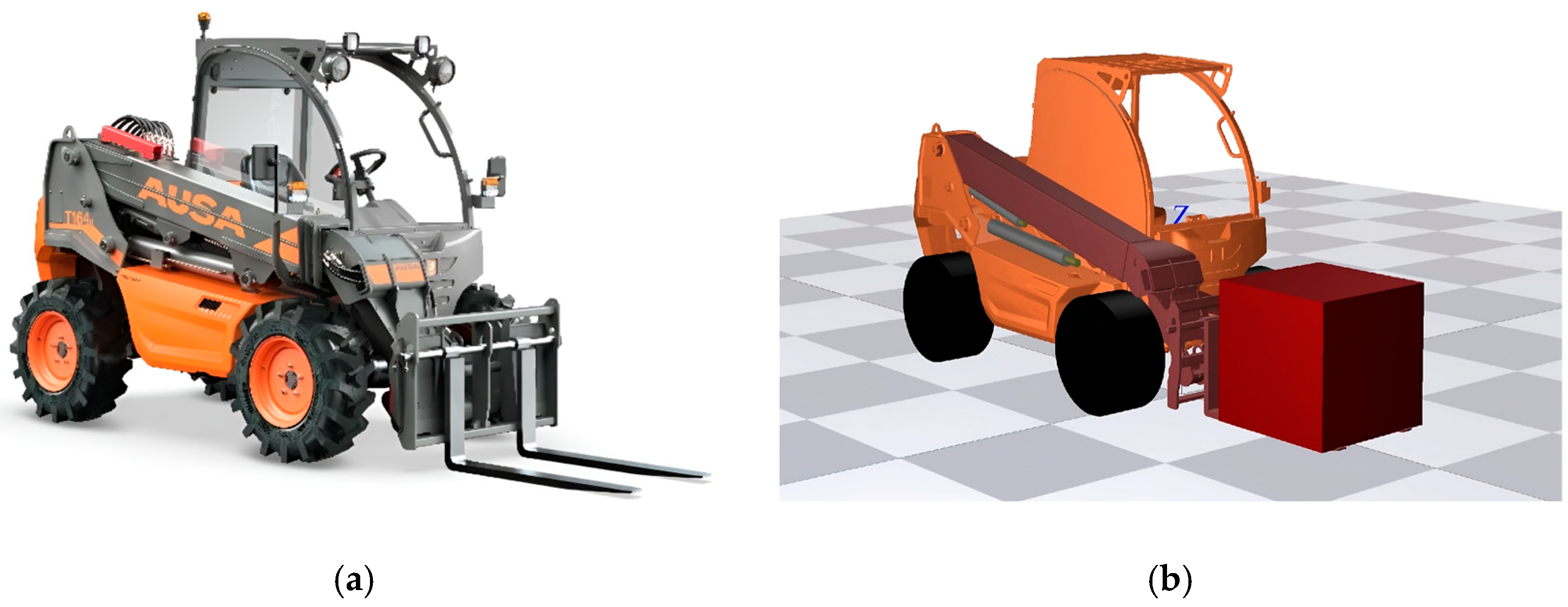
2.2. Model Description

According to the previous sections and the brief overview of the state of the art, which highlights the absence of models, even simple ones, that globally address all functionalities of compact hydraulic telehandlers, it is essential to develop a sufficiently detailed model that can serve as a simulation tool. In this context, two approaches can be adopted in the design and simulation of mobile hydraulic systems: one that is detailed and captures specific physical phenomena, and another that is more simplistic, prioritising modelling efficiency without sacrificing accuracy. The authors have chosen this second philosophy, considering it more suitable for small- and medium-sized mobile machinery, particularly in applications with telescopic arms.

Our proposed model will not only allow for the analysis of the dynamic behaviour of these machines but will also facilitate the optimisation of their performance. The following is a brief description of the mentioned machine, the identification of the strategy to be followed, and the establishment of some initial hypotheses.

In its original configuration, a compact hydraulic telehandler has a minimum of eight degrees of freedom. It consists of a platform with a fixed front axle and a pivoting rear axle. Mounted on the platform is a telescopic arm with a fork or other attachment at its end, as can be seen or inferred in Figure 1.

As an off-road vehicle, the telehandler has three primary degrees of freedom: forward/backward movement, turning, and rear axle pivoting to maintain stability on uneven ground. Additionally, the telescopic arm provides three more DOF: lifting, extending, and tilting the attachment at its end. To enable the arbitrary positioning and orientation of specialised end-effectors, two extra joints have been added at the end of the arm. However, these additional two DOF are not yet implemented in our first virtual model.

As a special feature in the functionality of lifting machines, lift and fork tilt movements are connected by an additional self-levelling circuit, also referred to as a hydraulic parallelogram circuit, as explained in the hydraulic circuit modelling section. This configuration allows the motion of the lift axis to drive the compensating (slave) cylinder, ensuring that the handler’s forks remain horizontal during the telescopic lift without needing to control the tilt axis.

When the telehandler is stationary but lifting or lowering a load, or when it is operating on rough terrain, it naturally experiences additional movements: (i) roll or side tilt: The platform leans to the side on uneven surfaces, affecting lateral stability; and (ii) pitch or forward–back tilt: The machine tilts forward or backward, affecting longitudinal stability. Additionally, the wheels are driven by a hydraulic transmission powered by a diesel engine or by an electric motor, providing another degree of freedom for movement.

When comparing the two primary methods for analysing the kinematics and dynamics of off-road machinery, the Newton–Euler method is generally favoured over the Lagrange method. This preference arises from its ability to provide comprehensive details about all links and joints, which is advantageous for later stress and performance assessments of components in operation. As noted in Craig, 2005 [39], the Newton–Euler formulation demonstrates at least a twofold increase in efficiency compared to the Lagrange approach in the context of a six DOF manipulator. Consequently, the dynamic analysis in this study utilised the Newton–Euler formulation. The Euler junction structure is applied, which defines the governing equations for the dynamics of bodies in large motion.

The compact hydraulic telehandler is represented as a sequence of a finite number of rigid bodies, interconnected by arbitrary joints. It may exhibit properties of rotational or translational degrees of freedom, and also damping and compliance, and normally contains some sort of attachment for drives and external forces. Therefore, a DAE (differential algebraic equation) system arises from its discretisation, with the algebraic equations coming mainly from constraints.

To determine the spatial motion of the rigid body, the well-known Euler equations are used. The first one represents the conservation of linear momentum, written as follows:

$$\sum \overrightarrow{F}={\displaystyle \frac{d\overrightarrow{p}}{dt}}={{\displaystyle \frac{d\overrightarrow{p}}{dt}}}_{│rel}+\overrightarrow{w}\times \overrightarrow{p}$$

(1)

where $\overrightarrow{F}$, $\overrightarrow{w}$, and $\overrightarrow{p}$ represent the external forces, the angular velocity vector, and the linear momentum vector, respectively; d/dt and d/dt_rel represent the derivative respect to the inertial frame and the derivative respect to the body-attached frame.

The second of the Euler equations sets up the conservation of angular momentum:

$$\sum \overrightarrow{M}={\displaystyle \frac{d\overrightarrow{h}}{dt}}={{\displaystyle \frac{d\overrightarrow{h}}{dt}}}_{│rel}+\overrightarrow{w}\times \overrightarrow{h}$$

(2)

where $\overrightarrow{M}$ and $\overrightarrow{h}$ represent the external torque and the angular momentum vector.

The port variables of the above model are defined with respect to the system attached to the centre of mass of the rigid body. Referring these port variables to the coordinates of interconnection with other bodies allow the coupling of the whole model. The port variables of two arbitrary points ‘A’ and ‘B’ of a given spatial body transform each other. The equations relating the linear and rotational efforts are the following:

$$\overrightarrow{M}=\overrightarrow{F}\times \overrightarrow{r}$$

(3)

For the flow variables, the equations are the following:

$$\overrightarrow{v}=\overrightarrow{w}\times \overrightarrow{r}$$

(4)

To transform the dynamic equations from those expressed in the body-attached frame of reference (roll, pitch, and yaw axes) to a spatially fixed frame of reference (X, Y, Z: inertial frame), it is necessary to choose some parameterisation for the rotations. Here, the global (inertial) reference frame, XYZ, is placed on the ground under the front axle. Initially, the global X-direction is longitudinal with respect to the vehicle, the Y-direction is lateral, and the Z-direction is vertical.

Among the multiple possibilities, Euler angles are used. To transform these rotations, the following equations are used:

$${\overrightarrow{w}}^{″}=\overline{\varphi }\overrightarrow{w}$$

(5)

$${\overrightarrow{w}}^{\prime }=\overline{\theta }{\overrightarrow{w}}^{″}$$

(6)

$${\overrightarrow{w}}^G=\overline{\psi }\overrightarrow{w^{\prime }}$$

(7)

$${\overrightarrow{v}}^{″}=\overline{\varphi }\overrightarrow{v}$$

(8)

$${\overrightarrow{v}}^{\prime }=\overline{\theta }{\overrightarrow{v}}^{″}$$

(9)

$${\overrightarrow{v}}^G=\overline{\psi }\overrightarrow{v^{\prime }}$$

(10)

where

$\overline{\varphi }=\left[\begin{array}{ccc}1& 0& 0\\ 0& \mathrm{c}\mathrm{o}\mathrm{s}\varphi & -\mathrm{s}\mathrm{i}\mathrm{n}\varphi \\ 0& \mathrm{s}\mathrm{i}\mathrm{n}\varphi & \mathrm{c}\mathrm{o}\mathrm{s}\varphi \end{array}\right]$	$\overline{\theta }=\left[\begin{array}{ccc}cos\theta & 0& sin\theta \\ 0& 1& 0\\ -\mathrm{s}\mathrm{i}\mathrm{n}\varphi & 0& cos\theta \end{array}\right]$	$\overline{\psi }=\left[\begin{array}{ccc}\mathrm{c}\mathrm{o}\mathrm{s}\psi & -\mathrm{s}\mathrm{i}\mathrm{n}\psi & 0\\ \mathrm{s}\mathrm{i}\mathrm{n}\psi & \mathrm{c}\mathrm{o}\mathrm{s}\psi & 0\\ 0& 0& 1\end{array}\right]$
$\overrightarrow{w}=\left[\begin{array}{c}{w}_x\\ w_y\\ w_z\end{array}\right]$	${\overrightarrow{w}}^{\prime }=\left[\begin{array}{c}{w^{\prime }}_x\\ {w^{\prime }}_y\\ {w^{\prime }}_z\end{array}\right]$	${\overrightarrow{w}}^{″}=\left[\begin{array}{c}{w^{″}}_x\\ {w^{″}}_y\\ {w^{″}}_z\end{array} \right]$	${\overrightarrow{w}}^G=\left[\begin{array}{c}{w}_x\\ w_y\\ w_z\end{array}\right]$
$\overrightarrow{v}=\left[\begin{array}{c}{v}_x\\ v_y\\ v_z\end{array}\right]$	${\overrightarrow{v}}^{\prime }=\left[\begin{array}{c}{v^{\prime }}_x\\ {v^{\prime }}_y\\ {v^{\prime }}_z\end{array}\right]$	${\overrightarrow{v}}^{″}=\left[\begin{array}{c}{v^{″}}_x\\ {v^{″}}_y\\ {v^{″}}_z\end{array}\right]$	${\overrightarrow{v}}^G=\left[\begin{array}{c}{v}_x\\ v_y\\ v_z\end{array}\right]$

The local geometry of the bodies refers to the position and orientation of the joints relative to the local reference frame. The inertia parameters specify the inertial properties of the bodies, including the position of the centre of gravity (CG), the mass, and the elements of the inertia tensor.

The multibody model is integrated with various submodels, such as a hydraulic model, a contact model, and a tyre friction model, to produce a more realistic mobile vehicle simulation.

Hydraulic systems can be modelled using lumped volume theory. When this theory is applied, it assumes that the effect of acoustic waves is negligible. In the lumped volume approach, the hydraulic circuit is divided into volumes within which pressure is assumed to be evenly distributed. Differential equations are established for these volumes to determine the system’s pressure (principle of conservation of mass, also referred to as the continuity equation). The various volumes through which fluid can flow are separated by throttles, and the flow rate is determined based on the pressure difference (the principle of conservation of energy, expressed as the Bernoulli equation).

The differential equation for hydraulic pressure at each volume i can be defined as follows:

$$\dot{p_i}={\displaystyle \frac{B_{ei}}{V_i}} \left(Q_{in,i}-Q_{out,i}-{\dot{V}}_i\right)$$

(11)

where Q_in,i and Q_out,i are the incoming and outgoing flow rates at volume i and V_i is the change in volume V_i with respect to time, respectively. In Equation (11), B_ei is the effective bulk modulus at volume i. The effective bulk modulus accounts for the bulk modulus of the fluid, the flexibility of container, and dissolved air.

The volume flow t Q in a generic restrictor can be written as follows:

$$Q_t=C_d A_t \sqrt{{\displaystyle \frac{2\left(P_{in}-P_{out}\right)}{\rho }}}$$

(12)

where C_d is the discharge coefficient, A_t is the cross-section area of the valve, $\rho$ is the density of the fluid, P_in is the input pressure, and P_out is the output pressure.

Contact modelling is an important modelling element when analysing real multibody systems. In scenarios involving collisions, where d_p is defined as the penetration distance at the point of contact, a spring-damper system is incorporated at this point to model the contact forces. The normal contact force, denoted as F_n, at the contact location can be expressed as follows:

$$\overrightarrow{F_n}=-\left(K d_p+C v_n\right) \overrightarrow{n}$$

(13)

where K_dp and C_vn represent the stiffness coefficient and the damping factor, respectively. The precise values of these two coefficients, K and C, are crucial, as they can lead to various types of desired collision responses. While the penalty method can closely approximate the actual contact conditions, its effectiveness is highly contingent upon the choice of penalty parameters and the specific circumstances involved.

Hypotheses and Considerations in Telehandler Modelling:

1. Arm Component Rigidity: All solids in the telehandler arm are considered rigid bodies. Previous experimental tests conducted at 100 samples/s identified two main natural frequencies: one at 37 Hz due to diesel engine vibrations and another related to the mass of the telehandler and the elasticity of the rubber wheels. This validates the rigid-body assumption, as the arm’s movement frequency, in the worst case, is two orders of magnitude lower than the first natural frequency.

2. Interaction between Components: Contact modelling plays a crucial role in analysing this multibody system. It has been applied to the hydraulic cylinder submodels, specifically when the piston reaches the end stop with the cylinder guide. Another relevant case is the valve-closing interaction, as in the overcentre valve, between the obturator and the seat. Additionally, the interaction between the rear pivoting axle and the platform has also been considered.

3. Friction Conditions: Friction conditions were implemented in three key areas: ground/tyre interaction using a simplified Pacejka model, the sealing system in hydraulic cylinders, and the telescopic guides of the lifting arm. Viscous friction models were used as an initial approach for the latter two cases. Given that this paper only analyses longitudinal stability due to the upward and downward movement of the load with the vehicle when stationary, the soil/tyre model has no significant effects, except for the vertical components of tyre elasticity and damping.

4. Damping Modelling: Damping is crucial for analysing vehicle vibration and dynamic response. Two relevant points are the damping in the hydraulic circuit, assuming constant oil compressibility, and tyre damping, which have been discussed in the text.

5. Mass Distribution: The mass distribution and inertia tensor of each component were calculated adequately due to their impact on system dynamics. At this point, we would like to mention an exception made for the mass placed on the fork. In the experimental phase, a cubic lattice structure was used, within which weights were added to simulate masses of 640, 1000, and 1600 kg. In the model, this mass was simulated as a homogeneous cubic volume but with variable density, depending on the load intended for testing.

6. Operating Conditions and Loads: The model was developed with anticipated loads and vehicle operating conditions, such as rough terrain and slopes, in mind, as the project’s objective is to study telehandler stability. However, in this first paper, the loads and conditions considered are limited to lifting movements (load raising and lowering).

3. Telehandler Modelling Using Scalar and Vectorial Bond Graphs

The bond graph invented in 1959 by Prof. H. Paynter (MIT) is a graphic language particularly suited for modelling multidisciplinary dynamic engineering systems Borutzky W., 2010 [40]. Utilising a unified symbology, it serves as an object-oriented modelling language that excels in describing the energy topology of a model at an acausal level through systematic processing.

The bond graph language offers several key advantages: (i) modularity, facilitating the development of complex models by allowing the independent design and analysis of components; (ii) maintainability, ensuring that its organised structure makes models easier to understand, modify, and maintain; and (iii) scalability, enabling the construction of larger, more complex models by combining simpler components.

Several symbolic software codes oriented to bond graph can be made available. Among them, we can highlight 20-SIM™, Amesim™, Bonsim, Bondyn, Symbol2000, and Modelica. Romero Rey G., in his thesis in 2005, summarised them [41].

The multi-bond or vector bond graph technique is applied in multibody theory to create a dedicated multi-bond graph library, as show by Bos A. M., 1986 [42]. It expands on the traditional bond graph method, using vector bonds and transforming elements into multiports. By doing so, bond graphs can be effectively utilised for analysing three-dimensional multibody systems. Tiernego M.J.L. and Bos A.M., 1985 [43], present a modular approach based on Newton–Euler equations and Hamiltonian formalism. Karnopp D. et al., 1976 [44], already proposed a procedure for constructing bond graphs using Lagrange equations. Different causality assignment procedures have also been proposed in the literature; see Marquis-Favre M. and Scavarda S., 2002 [45]. Library models for a rigid body and for various types of joints have been provided by Zeid A. and Chung C.H., 1992 [46], Cellier F. E. and Nebot A., 2005 [47], Zimmer, D. 2006 et al. [48], Filippini G. et al., 2007 [49], and Boudon B. et al., 2019 [50], so that bond graph models of rigid multibody systems can be assembled in a systematic manner.

Considering the previous sections, there are numerous software options available for modelling multi-solid systems based on bond graph methodology. We used the 20-SIM program for the numerical solution and simulation of the proposed model for the following significant reasons. First, we have accumulated substantial experience in recent years with the 1D and 3D bond graph methodology of De las Heras S. and Codina E., 1997 [51]. As part of his thesis, one of the authors, Filippini et al. in 2007, developed a multi-bond graph library for multibody systems, focusing specifically on accurately representing 3D dynamics, as can be seen at Figure 4.

Secondly, 20-SIM has the capability to simulate multi-solid systems without the need for additional tools. It is an interactive tool where model entry and model processing are fully integrated, allowing for real-time checks on model consistency during the entry and editing phases; see Marquis-Favre et al., 2002 [45]. The ability to use models in a plug-and-play fashion provides the modeller with significant advantages.

Furthermore, the resulting set of equations derived from a Bond Graph model consists of first-order ordinary differential equations (ODEs) supplemented with algebraic constraint equations (DAEs). These equations can be simulated using standard numerical integration methods. In our case, the Modified Backward Differentiation Formula was employed, ensuring that both absolute and relative integration errors are bounded at 0.0001. The initial step size was set to 1 × 10⁻¹² s, with a maximum allowable step size of 0.001 s, thereby optimising the accuracy and stability of the simulation.

The same figure illustrates the power bonds required to connect the submodels corresponding to the front wheels, the telescopic arm, and the rear axle, using the icons associated with the transformations required by the translations (T). The coloured frames of the submodel indicate which other submodels they are linked to.

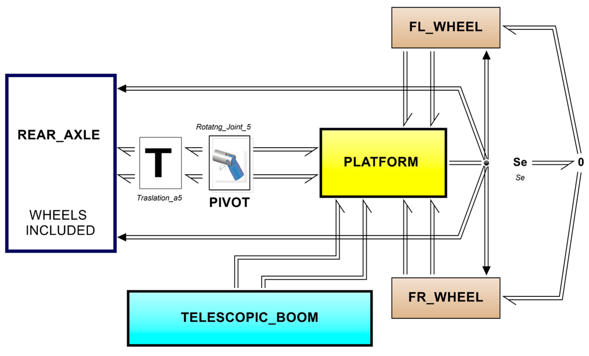
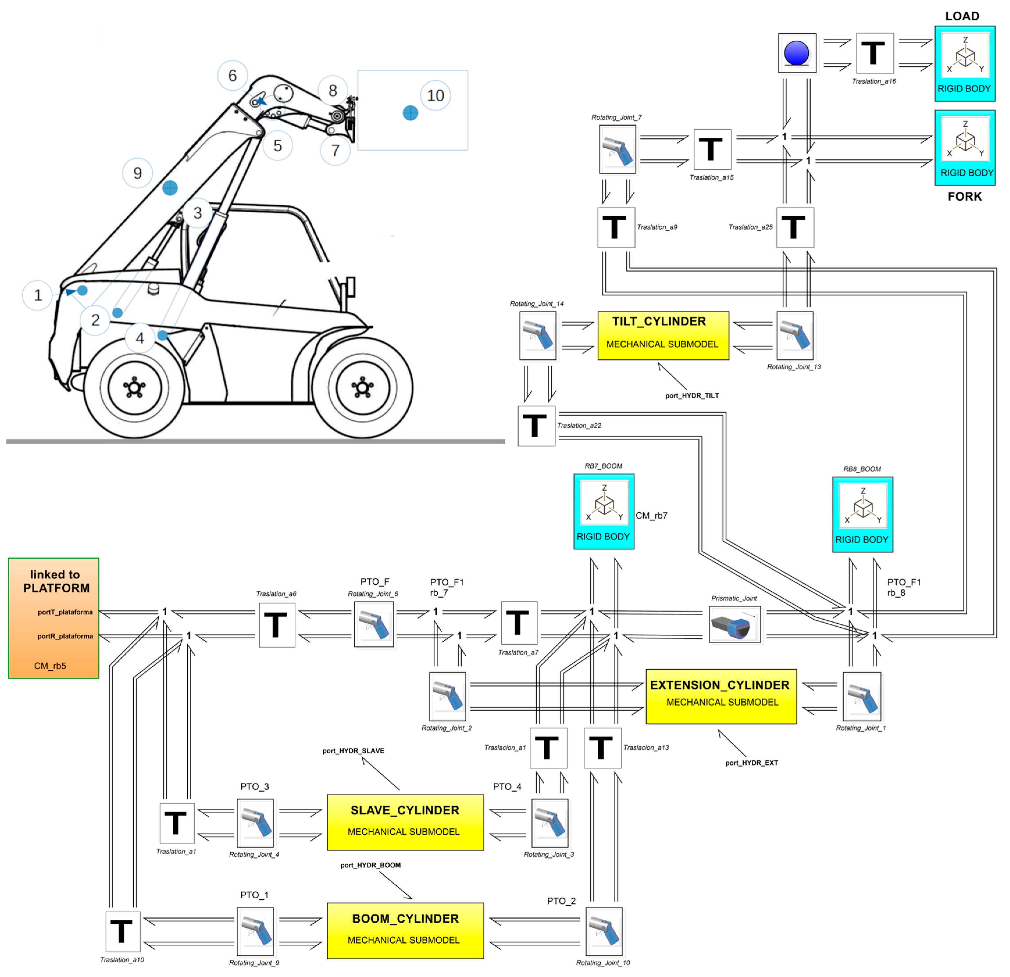
3.1. Telehandler Model (3D Bond Graph)

Most of the mechanical systems involved in the vehicle (platform chassis, rear axle, telescopic boom and attachment, and four wheels) require a three-dimensional treatment to solve their spatial dynamics. In this first paper, we have considered that two domains stand out in the machine under study: the mechanical part and the hydraulic part that drives the arm and attachments.

Mechanical Domain Modelling

To address the system’s complexity, it is organised as a hierarchical structure of layered submodels, where the foundational layer is consistently represented by the equations that configure the model.

The 3D model of the BG compact hydraulic telehandler, created in 20-SIM v.5, is presented in Figure 5. This model corresponds to the top layer of the virtual model structure. The mobile platform submodel is connected to the other submodels (for example, the telescopic arm submodel) through double multiport power bonds. Graphically, when the bonds are drawn in a horizontal position, the upper power bond corresponds to translational efforts and flows, and the lower power bond corresponds to rotational efforts and flows. If the bonds are drawn in a vertical position, the bonds on the left correspond to translational quantities, and those on the right correspond to rotational quantities. The port variables of each submodel are defined with respect to the system attached to the centre of mass of the rigid body. By referencing these port variables to the interconnection coordinates with other bodies, it is possible to couple them using the transformations icons R (rotations) and T (translations). Note that the drivetrain is simulated by a simple Se element (effort source). The double-arrow line is used to connect signals, as opposed to power bonds. In the figure, the double-arrow line transmits the velocity components of the platform to the wheel submodels (information required by the Pacejka formula).

• Platform submodel

The platform is configured with a series of components, including the structural chassis, cab, dashboard, engine, front axle, transfer case, oil reservoir, counterweights, drives, and other auxiliary supports. Figure 6 shows the platform submodel, where the main icon corresponds to the platform, modelled as a rigid body with a local coordinate reference frame (x, y, z) attached to the centre of mass and aligned with the principal inertia axes.

The mass equivalent of the platform is calculated by summing the masses of its components. The centre of mass of the platform is determined by considering the position and mass of each component, using the centre of mass formula for a discrete system. The moment of inertia for each component is calculated using specific formulas for its geometry, applying the parallel axis theorem when necessary. Next, the inertia matrix of the platform is formed, accounting for the contributions of all its components, and its eigenvalues are calculated to obtain the principal moments. These parameters are necessary to apply the Euler equations.

2.

Rear Axle submodel

The rear axle of a telehandler is a crucial component that supports the rear of the vehicle. It is designed to work in conjunction with the front axle (inserted in the platform submodel) and the vehicle’s steering and drive systems. This ensures optimal performance, especially in challenging working conditions. The combination of the steering cylinder, pivoting axle, spindles, and knuckles allows the telehandler to handle heavy loads, manoeuvre effectively, and maintain stability on uneven or rough terrain.

The rear axle submodel and the steering system submodel are shown in Figure 7. In the figure, the icons representing five rigid solids can be observed, corresponding to the rear axle, the two knuckles, and the hydraulic cylinder of the steering system. This component has been modelled using two rigid solids: one represents the body of the hydraulic cylinder, attached to the axle, and the other represents the double-acting piston. It is important to note that the linkage between these two parts has been made using a prismatic joint and a 1D bond that enables the connection between the mechanical and hydraulic domains.

Additionally, there are four joints of the rotation joint type, which correspond to the connections between the axle and the knuckles, as well as between the rods of the hydraulic cylinder and the steering bar that is part of the knuckle. These joints provide the necessary mobility and flexibility in the system. Furthermore, the two yellow frames correspond to the links to the wheel submodel.

3.

Wheel and Soil/Tire Interaction Submodel

This 3D-BG submodel in Figure 8 specifically addresses the wheel assembly (axle, rim, and tyre) and its interaction with the ground. The wheel is treated as a rigid body, with drivetrain effects not simulated; instead, an Se (Source of Effort) element injects torque into the wheel axle. This rigid body icon is linked to the white frame (representing the rear axle’s corresponding spindle/knuckle in Figure 8 through a rotating joint.

Two transformations are applied: a rotational (R) transformation aligns the local coordinate system with the global system, and a translational (T) transformation shifts the local coordinates of the rigid body to the tyre-ground contact point, using the tyre radius as a module.

The soil/tyre interaction models the tyre as a nonlinear system with multiple inputs (slip, angles, and load forces) and outputs (longitudinal/lateral forces and tyre moments). To define the “black box” linking these inputs and outputs in both steady and transient conditions, we apply Pacejka’s Magic Formula Tire model [52]. This model is fed with the platform’s translational velocity, the velocity at the tyre-ground contact point, and the rotational variables of the wheel axle.

A ‘C’ component and an ‘R’ component account for tyre stiffness and damping, with parameter values discussed in Section 4. The soil profile is represented as a virtual horizontal plane, with axes aligned to the model’s absolute axes.

4.

Telescopic arm system

In Figure 9, the submodel of the telescopic arm is shown, configured from basic 3D-BG elements. The rigid solid icons correspond to the fixed arm, telescopic arm, fork, and load. It is worth highlighting the icon of a translational joint to simulate the relative movement between the fixed arm and the telescopic arm.

Each of the hydraulic cylinder submodels (yellow frames) are configured according to the structure outlined in Figure 10. These icons are linked with the rigid solids through the corresponding revolute joints. It is important to note that to ensure stability during operation, a hydraulic parallelogram-type self-levelling system is included, which requires the incorporation of a slave hydraulic cylinder. The hydraulic connection between the slave cylinder and the tilt cylinder is explained at Figure 11 and in Section 4.2. at the Hydraulic Domain.

Figure 10 presents an approach to the modelling of a hydraulic cylinder that appears innovative based on the literature reviewed in the references section. In Figure 10a, a typical hydraulic cylinder is illustrated, characterised by a single rod and a double-acting design. Figure 10b shows the 3D-BG schematic, emphasising the mechanical aspect of the cylinder. The rigid solid icons representing the cylinder’s body and the rod/piston assembly are connected by a translational joint, simulating their relative movement. Figure 10c details the internal structure of the prismatic joint, which differs slightly from that shown in Figure 4, as it requires the injection of the variables (effort and flow) that define the energy rate of the relative movement, deduced from the hydraulic domain, as explained in the 1D-BG bond graph in Figure 10d and Figure 12. Additionally, a model has been incorporated to simulate the collision between the piston and the cap-ends of the cylinder casing when the piston reaches either end of its stroke. Regarding Figure 10b,d, the friction resulting from the relative movement of the cylinder’s components has been simulated using a black box that follows the Karnopp or Stribeck model, although this first paper only considers viscous friction. This approach allows for a more precise modelling of the hydraulic cylinder’s dynamic behaviour, integrating both mechanics and hydraulics into a single model.

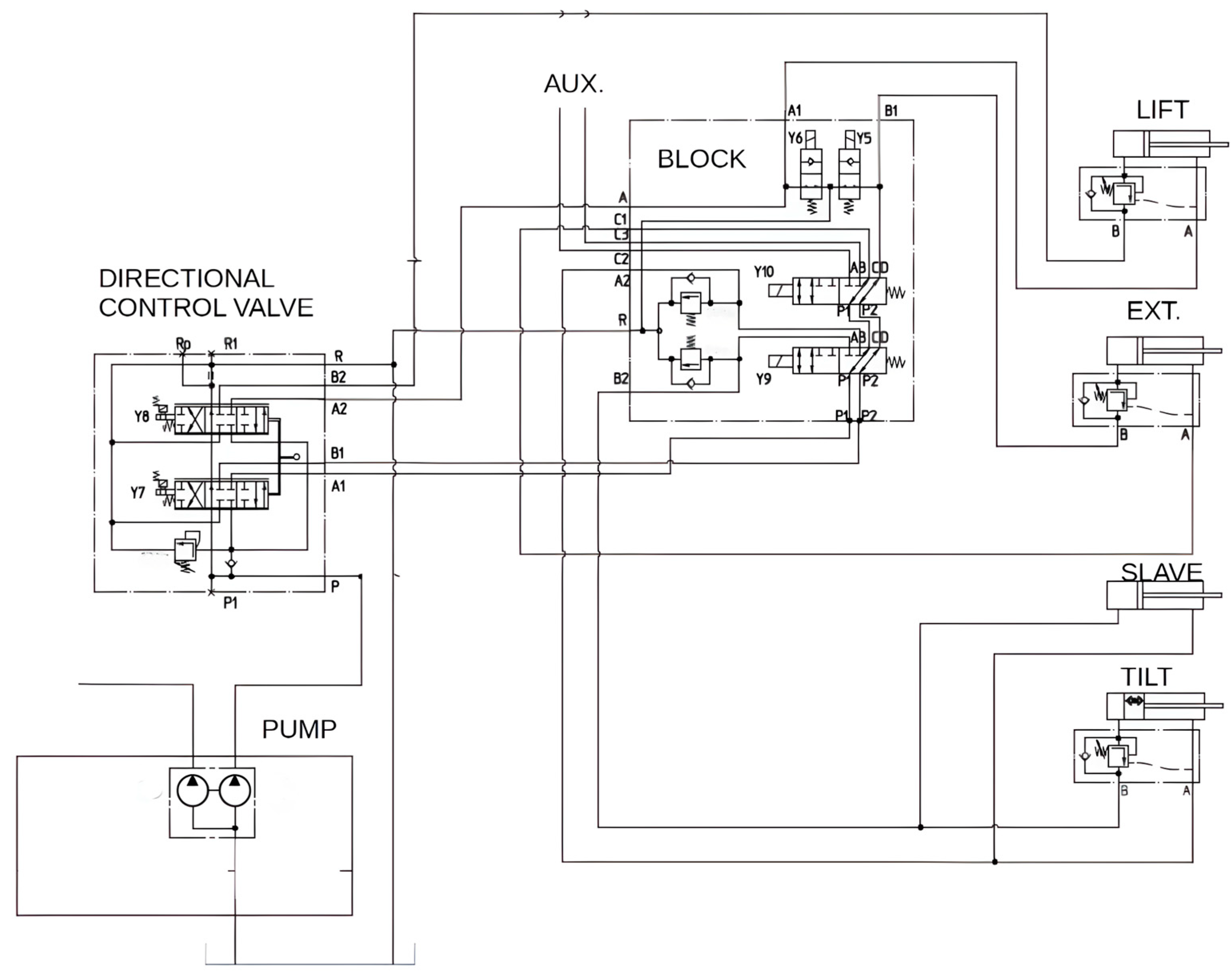
3.2. Hydraulic Domain Modelling

The modelling of the hydraulic systems configuring the telehandler, referred to as the hydraulic domain, can be accurately performed using basic bond graph elements. These elements are characterised by 1D bonds that are defined by two scalar variables: the effort variable, which represents pressure, and the flow variable, which represents flow rate.

In a telehandler, we can distinguish three hydraulic subsystems: the rolling transmission subsystem, the steering subsystem, and the arm/implement drive subsystem. However, in this paper, we only consider the implement drive subsystem of the boom/fork assembly given that it decisively affects the dynamic behaviour of the machine. The basic schematic is shown in Figure 11.

In this diagram, we highlight the following basic components: the pump group represented by the pump and a pressure relief valve, the open-centre directional control valve (two-spool), a valve block which can be referred to as a safety block, and the hydraulic cylinders responsible for the lifting, extension, and tilting.

To be as clear as possible, we have decided to explain the modelling process only for the circuit corresponding to the lifting movement of the arm, considering that the others are very similar and explaining them all would be redundant.

The corresponding bond graph schematic is shown in Figure 12. In this figure, we highlight the bond graph diagram of the hydraulic cylinder, in which two transformer elements, TF, are used: one converts pressure and flow rate to linear motion and force (representing the chamber connected to the pressure line), and the other converts linear motion and force to pressure and flow rate (modelling the connection of the chamber to the return line). The 1-junction represents a coupling where all the flows of the connected bonds are equal. The submodel “end stop” aims to represent the contact forces when the piston comes into contact with the guide plug or the cylinder cap. The modelling also includes the compressibility of the fluid in the two cylinders chamber, the effects of friction (only viscous term), and the inertia due to the moving mass of the cylinder piston and rods. Finally, the equivalent load is simulated as a negative effort (force) exerted at the cylinder rod tip from the boundary.

The flow variable in this bond, denominated as the “hydraulic port”, is the rod velocity, which connects with the 3D bond graph of the mechanical domain that simulates the hydraulic cylinder actuating the boom (see Figure 13 and Figure 14).

We also want to highlight the inclusion of a load-holding valve in this circuit, also known as an overcentre valve, and its corresponding check valve. Load-holding valves are used with cylinders to safely hold suspended loads and manage over-running loads.

Figure 14 shows in detail the generic bond graph of an overcentre valve, which is customised for the case of the valve CEB1 with atmospheric drainage. Here, the most significant parts are the four MTF elements that transform the effect of pressure on the different effective sections of the poppet into forces that combine at the 1-junction; the “flow forces” submodel (momentum conservation theorem) and forces due to spring compression have been included [53

The 1-junction represents a force balance and is a generalisation of Newton’s third law. From here, we can determine the kinematic variables of the shutter and, consequently, deduce the relative position using the internal geometry of the valve. Since the relative position between the poppet and its seat defines a passage section, we can calculate the flow rate through it by applying Bernoulli’s equation. The discharge coefficient has been used here as an empirical correlation, a function of the Reynolds number and the geometry of the passage section defined by the relative position. This is included inside of the “orifice” submodel [53]

As mentioned in a previous section, the lift and tilt actuation are managed by two six-way three-position mono-block directional valves. In the neutral position, both valves connect the pump port to the tank port. If either valve shifts from neutral, the pump disconnects from the tank. This configuration can be represented by combining orifices with variable area (metering) and a check valve block. When the valve is neutral, all orifices overlap except $PT1 \mathrm{and} PT2$. These two orifices start the simulation with an opening offset (underlapping), allowing the pump to deliver low-pressure flow to the tank.

Figure 14 illustrates the basic connection diagram, while Figure 15 shows the bond graph diagram, highlighting the different metering sections between ports P, T, A, and B and its control. The flow rate through the metering orifices depends on the opening area and the pressure drop across the valve. If ΔP is the pressure drop and A(x) is the metering section area (based on spool position x), the volumetric flow rate Q can be calculated as $Q=Cd\ast A\left(x\right)\ast \sqrt{\mathsf{\Delta }}\mathrm{P}$, where Cd is the discharge coefficient. The discharge coefficients are derived from fitting a quadratic polynomial to the experimental data of pressure drop versus flow rate, according to the methodology presented (Borghi [54]).

4. Experimental Test

After the construction of the model, it is imperative to subject it to rigorous validation, a crucial step that entails testing its performance against real-world data. This validation process typically involves evaluating the model’s response to empirical data and scrutinising its accuracy in comparison to observed values. While inertial and geometrical parameters of the mechanical system, including the hydraulic actuator components, can be readily obtained from the geometry, other parameters pose greater challenges. For instance, the elasto-damping parameters of the tyres and, particularly, verifying specific parameters of the hydraulic system and its components, can be more elusive.

In the mechanical domain, we utilised software tools such as Siemens-NX and Catia v6, made accessible through educational licences provided by the UPC. Our telehandler model, consisting of 22 rigid bodies, was methodically constructed using suitable kinematic joints. All pertinent parameters have been compiled in

Table 2. Multi-solid model and main geometric and dynamic parameters.

			CM (m)			Moment of Inertia, IIG (kg m2)
Rigid Body	Denomination	Mass (kg)	x	y	z	IIG1 (kg m2)	IIG2 (kg m2)	IIG3 (kg m2)
Left front wheel	RB1	40.0	0.000	0.628	0.360	1.0	1.0	2.2
Right front wheel	RB2	40.0	0.000	−0.628	0.360	1.0	1.0	2.2
Left rear wheel	RB3	40.0	−1.750	0.628	0.360	1.0	1.0	2.2
Right rear wheel	RB4	40.0	−1.750	−0.628	0.360	1.0	1.0	2.2
Platform (motor, axle, cardan, transfer box, oil tank, chassis)	RB5	2096.0	−1.250	0.014	0.710	121.0	1032.0	1085.0
Rear axle	RB6	113.0	−1.741	0.010	0.362	0.8	12.6	12.6
Boom	RB7	147.0	−0.809	−0.476	1.130	37.5	37.5	3.0
Mobile boom	RB8	165.0	−0.203	−0.383	0.927	76.0	76.0	6.4
Attachment (tablier, rocker, two forks)	RB9	178.0	0.938	0.000	0.102	2.0	2.0	3.5
Load	RB10	640.0	1.177	0.000	0.514	266.0	266.0	266.0
Housing lift cylinder	RB11	25.5	−0.805	−0.476	0.858	1.5	1.5	0.2
Piston lift cylinder	RB12	25.5	−0.805	−0.476	0.858	1.5	1.5	0.2
Housing compensation cylinder	RB13	9.0	−1.325	−0.476	1.079	0.3	0.3	0.1
Piston compensation cylinder	RB14	9.0	−1.325	−0.476	1.079	0.3	0.3	0.1
Housing flip cylinder	RB15	14.5	0.250	−0.260	0.611	0.3	0.3	0.1
Piston flip cylinder	RB16	14.5	0.250	−0.260	0.611	0.3	0.3	0.1
Housing steering cylinder	RB17	6.5	−1.872	0.000	0.439	0.3	0.3	0.1
Piston steering cylinder	RB18	6.5	−1.872	0.000	0.439	0.3	0.3	0.1
Left steering rod	RB19	2.0	−1.872	0.412	0.439	0.1	0.1	0.1
Right steering rod	RB20	2.0	−1.872	−0.412	0.439	0.1	0.1	0.1
Left carrier	RB21	3.0	−1.787	0.455	0.450	0.5	0.5	0.2
Right carrier	RB22	3.0	−1.787	−0.455	0.450	0.5	0.5	0.2

for reference.

In this section, it is emphasised that one of the primary challenges in developing the virtual model was estimating the tyre stiffness and damping coefficient parameters. Initially, the values reported by Lines J.A. in 1991 [55,56] were adopted and later compared with data provided by the tyre manufacturer (see Figure 16). Previous numerical values related to wheel vertical movement are summarised in Figure 17 (left), where it was determined that a tyre stiffness of 600 kN/m was more suitable for the virtual model. This choice was based not only on the manufacturer’s information but also on real-world tests, which indicated that vertical displacement did not exceed 5 mm.

Estimating the damping coefficient proved to be more challenging. When employing the coefficient proposed by Lines, the numerical results (see Figure 17 (right)) exhibited vibrational behaviour that did not align with empirical data. Through a trial-and-error approach, it was concluded that the damping coefficient needed to be increased by an order of magnitude to achieve greater fidelity in the model’s outcomes.

Turning to the hydraulic domain, each submodel has undergone validation by comparing numerical results with characteristic curves sourced from technical manufacturer catalogues. These comparisons have been conducted under conditions replicating those in which the characteristics were experimentally obtained in the manufacturers’ laboratories. Additionally, the most significant hydraulic parameters have been outlined in

Table 3. Hydraulic parameters.

Table (Hydraulic Parameters)	Value	Units
Oil density	875	kg/m3
Oil bulk modulus	17.500	bar
Oil kinematic viscosity	46	cSt
Pump maximum displacement	12	cm3/rev
Pump volumetric efficiency	0,93
Pump hydraulic–mechanical efficiency	0,96
Relief valve cracking pressure	210	bar
Overcentre valve ratio (CEB) (*)	4:1
Overcentre pressure setting	275	bar
Directional control valve block (*)	202	serie
Viscous friction coefficient	50	N/m/s
Cylinder leakage coefficient	0.01	L/min/bar
Piston diameter of the boom hydraulic cylinder	100	mm
Rod diameter of boom hydraulic cylinder	55	mm
Travel of boom hydraulic cylinder	689	mm
Piston diameter of the extension hydraulic cylinder	60	mm
Rod diameter of extension hydraulic cylinder	40	mm
Travel of extension hydraulic cylinder	1.239	mm
Piston diameter of the fork hydraulic cylinder	100	mm
Rod diameter of fork hydraulic cylinder	60	mm
Travel of fork hydraulic cylinder	268	mm
Piston diameter of the slave hydraulic cylinder	75	mm
Rod diameter of slave hydraulic cylinder	45	mm
Travel of slave hydraulic cylinder	344	mm
Engine power	19	kW
Torque	92.6/1700	Nm/rpm
Engine speed	2.300	rpm (max)

(*) The geometric parameters of hydraulic components have been determined experimentally in lab but we cannot disclose the values as they are proprietary to the manufacturers.

.

Given that all the work is aimed at a future detailed study on the global stability of this type of machinery, we have deemed that it is important first to validate the model based on the distribution of reaction forces on the four tyres at their contact with the ground and the self-levelling mechanism of the fork.

4.1. Experimental Methodology

In this section, the tests conducted with the AUSA T164 telehandler are described. The objective of these tests is to evaluate the validity of the model described in previous chapters and to deepen the understanding of the machine’s performance. The tests conducted have been grouped into two categories:

• Tests to determine the ground reaction forces on the four wheels under different operating conditions of the machine. The results of these tests will be used to validate the virtual model from a mechanical perspective.
• Tests on some specific functionalities of the machine, such as the self-levelling of the attachment fork. The experimental results will allow for the validation of the virtual model from a hydraulic perspective.

The test has been carried out under the EN 15000:2008 [4] standard and ISO 22915-14:2010 [5]. Figure 18 presents a general view of the instrumented prototype.

Table 4. List of sensors and equipment used.

Instrumentation	Characteristics	Reference
Position: 2 inclinometers	2 inclinometers (I) to measure fork levelling −45° to 45° and 4 to 20 mA	SICK TMM55E-PMH045
	3 extensometers (X) to measure boom extension. 0 to 1500 mm and 0 to 10 V	Micro epsilon, WDS-1500-P60-SR-U
Accelerometers: 7 accelerometers	7 lineal accelerometers, 3 axes, ranging from 3 g and 6 g	SparkFun, Triple Axis Accelerometer—MMA7260Q (6 g)/Analogue devices, ADXL335 Small, Low Power, 3-Axis ± 3 g
Loading: 2 weighing equipment	2 electronic weighing system with visor. Used to weigh vehicle’s axles and total weight. Composed of two portable platforms of the WWS series and weighing terminal with touch screen and integrated printer.	DINI ARGEO USBCKR-1, portable kit. Wired version
Flow: 1 flowmeter	A flowmeter (Q) 0 to 300 L/min., 4 to 20 mA	HYDAC EVS 3100-A-0300-000
Pressure: 13 pressure transducers (P)	13 pressure transducers (P) of two types: 3 of 0–400 bar and 10 of 0–250 bar. 4 to 20 mA	WIKA, MH3 with connector M12
Temperature: 1 sensor (T)	A PT 100 (T) temperature sensor and temperature transmitter (converts PT100 signal to a 4 to 20 mA electrical signal). Temperature transmitter ranges: 0 to 250 °C and 4 to 20 mA	Temperature transmitter model: Wika T20.10.100
Other analogue signals	Analogue input signals of Delta Equipment: Voltage signal from 0 V at low level and 10 V at high level	3 Triggers: one for the National Instruments Equip., one for the load cell, and one for the 3-way flow regulating valve solenoid signal

details the data acquisition and processing equipment used the sensors are listed in

Table 5. Data acquisition and processing equipment.

Experimental Equipment	Characteristics	Reference
Equipment 1 data acquisition	Equipment for accelerometer signals data acquisition	National Instruments USB-6343
Laptop 1	LabVIEW for acquisition of accelerometer signals	LabVIEW 2021 and NI software
Equipment 2 data acquisition	Data acquisition from hydraulic, position and temperature transducers and sensors	Delta RMC200
Laptop 2	Delta RMC Tools Software for acquisition signals from pressure, flow, temperature, and position sensors	Delta RMC Tools Software
Laptop 3	To acquire data from the rear axle load cell of machine
Digital camera	To record videos	Sony RX100 IV

.

Here, we would like to draw attention to the fact that electronic dual-channel scales were used to measure the load on each wheel of the telehandler, thus determining the reaction force. We had two portable platforms from the WWS series, which required us to repeat each test. In the first test, the scales were placed on the wheels on the arm side, and in the repetition, they were positioned on the opposite side. Furthermore, each test had a specific duration, primarily influenced by the variability in the lift and descent speeds, which were determined by the revolutions of the prime mover in the hydraulic circuit and the joystick positions, according to the previously established test plan.

Based on the above, it was necessary to non-dimensionalise the time scale to facilitate the comparison of ground reaction forces on each wheel and the analysis of the resulting graphs.

4.1.1. Tests to Determine the Ground Reaction Forces (Mechanical Domain)

The tests involve performing the movements of the telescopic boom, representing a normal service operation with the telehandler. Essentially, this consists of raising and lowering the boom, meaning elevating it and also extending the boom in various positions from the most retracted to the most extended (positions A, B, C, D, E, and F), with different loads on the fork. The extension between the different positions is 250 mm. The tests were conducted at two speeds: slow speed, approx. 1000 rpm (idle), and fast speed, 2220 rpm. The loads used were 0, 640, 1000, and 1600 kg. These loads correspond to the load capacity chart for the attachment being tested; in our case, this was a fork, in accordance with the requirements imposed by current safety standards. In this regard, we want to highlight that a significant portion of the tests have been conducted with a load of 640 kg, considering that with this load, all the movements permitted can be performed.

In Figure 19, the ground reaction force values at all four wheels during the boom’s lifting motion (both upward and downward) are presented. In these tests, the telescopic arm was fully retracted, and the load on the fork was 0 and 1600 kg. An initial reading of these data suggest that the behaviour during ascent and descent is very similar, and that the reactions on the rear wheels (Rear_Right (RR) and Rear_Left (RL)) are practically identical. The maximum and minimum values of the ground reaction forces as a function of the mass on the fork attachment are shown in Figure 20.

4.1.2. Tests to Determine the Functionality Performance (Hydraulic Domain)

From a hydraulic functionality perspective, we found it interesting to present the working conditions of the lift cylinder and the tilt cylinder under various operating conditions. For the hydraulic lift cylinder, Figure 21 shows the pressures on both sides of the hydraulic cylinder during the boom’s upward and downward movements.

The pressure traces P1 are a function of the load and position of the lifting cylinder, but also of the resistive force of the slave cylinder. The latter causes the slope of the curve to vary, as indicated in [15]. In addition, Figure 22 illustrates the operating values of the overcentre valve connected to the piston-side chamber of the cylinder on a (Px, P1) diagram, as described in [57]. These values are approximately aligned along a line (depicted by a blue dashed line) parallel to the characteristic curve of the overcentre valve. This alignment suggests that during a slow descent of the lift cylinder, the overcentre valve needs to open, facilitating a flow rate of around 20 L/min for the four load conditions when the telescopic arm is retracted. Moreover, different loading conditions are highlighted through parallel dashed lines on the characteristic curve of the cylinder.

One of the most important features of a telehandler’s performance is the fork attachment’s self-levelling capability. As illustrated in the hydraulics circuits diagrams, to achieve self-levelling, a slave hydraulic cylinder has been utilised, which is driven by the boom, itself actuated by the lift cylinder. The chambers of the slave cylinder are connected to those of the tilt cylinder (piston-side chamber to piston-side chamber, and similarly for the rod-side chambers). With this setup, the slave cylinder functions as a positive displacement pump.

4.2. Experimental vs. Numerical Results: A Critical Examination of Their Validity and Model Limitations

• Mechanical domain

In Figure 23 we can see the temporal evolution of the ground reaction forces on the wheels due to the lifting and lowering of a 1020 kg load with the telescopic boom in position E, which corresponds to a relative extension displacement of 1 m with respect to the fixed arm. These results were obtained through the developed 3D-BG virtual model. These graphs are an example of the numerous numerical simulations conducted, with the summarised results shown in the following figures.

This graph illustrates a key aspect of the telehandler’s longitudinal stability, highlighted by the minimum values reached by the rear wheel reaction forces. Clearly, a zero-reaction value would indicate vehicle overturning. Notably, peaks appear at the initiation and termination of the movement.

The information obtained can be used to establish the safety threshold for the load cell, which is installed as a safety element at a specific point on the rear axle. This threshold is critical for ensuring operational stability and preventing tipping under load.

Following the same order of presentation as the previous paragraph, a comparison between the results of the virtual model of the telehandler and the experimental results obtained during the tests is shown below. In order to cover the entire working range of the machine (both in lifting and extending), these comparisons have been conducted with a mass of 640 kg for the two positions of the extension arm: retracted (position A) and extended (position E).

In Figure 24, the experimental values (solid line) and numerical values (dashed line) are shown. To highlight the accuracy of the virtual model, Figure 25 shows the percentage error between the numerical and experimental values. It is calculated by dividing the absolute difference between them by the nominal load per wheel, defined as the total weight of the machine (including the load) divided by four. This quotient, expressed as a percentage, quantifies the precision of the numerical results relative to the experimental data. In general, the percentage differences are less than ±10%. Similarly, Figure 26 shows ground reaction forces (both experimental and numerical values) as a function of telescopic extension position with a 640 kg mass on the fork.

The discrepancies between the numerical and experimental results can basically be attributed to the following three aspects: Firstly, the experimental measurements; although the load cells used are highly precise, transferring data from the load cells to our acquisition system introduces an undesirable temporal error. This is evident in the graphs, which, instead of following a continuous line, appear as broken lines with step-like segments. Secondly, at the beginning and end of the movements, there is a certain disturbance caused by the same operator, which affects the readings of the load cells. Finally, the virtual model includes a platform comprising many elements, but it has been represented by a single rigid body with a centre of mass. Any small deviation in the coordinates of the centre of mass can introduce significant variations in the ground reaction forces.

2.

Hydraulic domain

Figure 27 depicts the numerical results (black line) showing the ratio between the speeds of the tilt cylinder and the slave cylinder, as well as the ratio based solely on the geometries of the two cylinders, represented by a blue line. Additionally, the red line indicates the theoretical model’s error in the fork’s inclination. To compare with the experimental ratios, it is noted that during testing, the levelling error for a load of 0 kg is within the range of ±0.25 degrees, while for a load of 1600 kg, the error oscillates between ±0.5 degrees. However, when several consecutive cycles are performed, such as five cycles, the errors increase to ±0.25 degrees for 0 kg and ±2 degrees for 1600 kg. These results underscore the effectiveness of the T164 telehandler’s hydraulic self-levelling system and its relationship to stability, as well as the precision of the numerical model outcomes.

5. Conclusions and Final Remarks

This study has introduced a foundational virtual model developed through multiphysics modelling using the bond graph (BG) methodology, which has proven to be particularly relevant to addressing the longitudinal stability of telehandlers. As outlined in the main contributions, this model was a vital tool during the pre-design and main design stages, offering essential insights into performance characteristics, especially in electrified versions.

The model encompasses the critical components necessary for accurately replicating the mechanical and hydraulic aspects of the vehicle, including the chassis, rear axle, telescopic boom, attachment fork, and wheels. A comprehensive three-dimensional treatment of these complex components has been employed to capture spatial dynamics effectively. Supported by experimental data, this demonstrates the model’s fundamental functionality, focusing on calculating wheel reaction forces and analysing the hydraulic self-levelling phenomenon of the attachment fork. Discrepancies of up to 10% have been noted as acceptable within a well-designed mechanical domain, while more precise models may be unnecessary given the significant variability in field operating conditions.

Thanks to BG-3D model simulations on the 20-SIM platform, the stability limits estimations have been satisfactorily proved.

In summary, this study emphasises the developed virtual model’s effectiveness in understanding and predicting telehandler dynamics. The modelling skills in mechanical and hydraulic aspects have been robust and experimentally validated. In our following paper, our aim is to use the virtual model to study the global stability of the machine under different working conditions.

The innovative application of multi-dimensional bond graph enhances modelling productivity and deepens the understanding of the system’s key physical attributes. The authors are committed to promoting the bond graph methodology in mobile machinery studies, recognising its potential to advance research and innovation. Importantly, this paper forms part of a broader project to strengthen collaborative research activities between the business and academic sectors, fostering advancements in electrified non-road mobile machinery (NRMM).

References

1. Priora, G. Monitor and Control System of the Dynamic Stability on a Telescopic Handler with Telemetry and Experimental Data. Master’s Thesis, Politecnico di Torino (Italy), Torino, Italy, 2019. [Google Scholar]
2. Machinery Regulation (UE) 2023/1230. Available online: https://eur-lex.europa.eu/eli/reg/2023/1230/oj (accessed on 14 June 2023).
3. CEN/TS 1459-8:2018 (MAIN); Rough-Terrain Trucks—Safety Requirements and Verification—Part 8: Variable-Reach Tractors. Asociación Española de Normalización: Madrid, Spain, 2018.
4. CEN/EN 15000:2008; Safety of Industrial Trucks. Self-Propelled Variable Reach Trucks. Specification, Performance and Test Requirements for Longitudinal Load Moment Indicators and Longitudinal Load Moment Limiters. Asociación Española de Normalización: Madrid, Spain, 2018.
5. ISO 22915-14:2023; Industrial Truck—Verification of Stability. Part 14: Rough-Terrain Variable-Reach Trucks. International Organization for Standardization: Geneva, Switzerland, 2023.
6. ISO 10896-1:2020; Rough-Terrain Trucks—Safety Requirements and Verification. Part 1: Variable-Reach Trucks. International Organization for Standardization: Geneva, Switzerland, 2020.
7. Safe Use of Telehandlers in Construction; Good Practice Guide, 2nd ed.; Reference No. CPA 1101; Construction Plant-Hire Association: London, UK; Health Safety Executive (HSE): Merseyside, UK, 2015.
8. Hunter, A.G.M. A review of research into machine stability on slopes. Saf. Sci. 1993, 16, 325–339. [Google Scholar] [CrossRef]
9. Bietresato, M.; Mazzetto, F. Stability Tests of Agricultural and Operating Machines by Means of an Installation composed by a Rotating Platform with Four Weighting Quadrants. Appl. Sci. 2020, 10, 3786. [Google Scholar] [CrossRef]
10. Urkullu, G. Integración de las Ecuaciones de la Dinámica de Sistemas Multicuerpo Mediante Diferencias Centrales de Orden dos. Ph.D. Thesis, Universidad del País Vasco—Euskal Herriko Unibertsitatea, Leioa, España, 2019. [Google Scholar]
11. Garcia-Vallejo, D.; Mayo, J.; Escalona, J.L.; Domínguez, J. Three-Dimensional Formulation of Rigid-Flexible Multibody Systems with Flexible Beam Elements; Multibody System Dynamics 20: Singapore, 2008; pp. 1–28. [Google Scholar]
12. Beater, P.; Otter, M. Multi domain simulation: Mechancis and hydraulics of an excavator. In Proceedings of the Conference: 3rd International Modelica Conference, Linköping, Sweden, 3–4 November 2003; The Modelica Association: Linköping, Sweden, 2003. [Google Scholar]
13. Patil, A.; Radle, M. Hydraulic and multibody combined simulations for electric forklift design using modelica. Int. J. Eng. Sci. Technol. 2022, 10, 27–35. [Google Scholar] [CrossRef]
14. Altare, G. Analisi e Modellazione del Circuito Idraulico di un Miniescavatore. Master’s Thesis, Politecnico di Torino, Torino, Italy, 2009. [Google Scholar]
15. Altare, G.; Lovuolo, F.; Nervegna, N.; Rundo, M. Coupled Simulation of a Telehandler Forks Handling Hydraulics. Int. J. Fluid Power 2012, 13, 15–28. [Google Scholar] [CrossRef]
16. Casoli, P.; Alvin, A. Modelling of an Excavator Pump Nonlinear Model and Structural Linkage/Mechanical Model. In Proceedings of the 12th Scandinavian International Conference on Fluid Power, Tampere, Finland, 18–20 May 2011; pp. 25–40. [Google Scholar]
17. Prabhu, S.M. Model-Based Design for Off-Highway Machine Systems Development; SAE: Warrendale, PA, USA, 2007. [Google Scholar] [CrossRef]
18. Jhala, H.S. A Multibody Simulation Approach to Identify Critical Instability Scenarios of a Forklift Truck. Master Automotive Technology. Master’s Thesis, Eindhoven University Technology, Eindhoven, The Netherlands, 2023. [Google Scholar]
19. Hong, T.D.; Pham, M.Q.; Tram, S.C.; Tram, L.Q.; Nguyen, T.T. A comparative study on kinetics and dynamics of two dump truck lifting mechanisms using Matlab Simscape. Theor. Appl. Mech. Lett. 2024, 14, 100502. [Google Scholar] [CrossRef]
20. Roccatello, A.; Mancò, S.; Nervegna, N. Modelling a Variable Displacement Axial Piston Pump in a Multibody Simulation Environment. J. Dyn. Sys. Meas. Control 2007, 29, 456–469. [Google Scholar] [CrossRef]
21. Sapietova, A.; Saga, M.; Novak, P. Multi software platform for solving of multibody systems synthesis. Commun. Sci. Lett. Univ. Zilina 2012, 14, 43–48. [Google Scholar] [CrossRef]
22. Prescot, W. Using multibody dynamics solvers in a Multiphysics environment. Multibody Dynamics. In Proceedings of the ECCOMAS Thematic Conference, Warsaw, Poland, 29 June–2 July 2009. [Google Scholar]
23. Zi, B.; Zhang, L.; Zhang, D.; Qian, S. Modelling, analysis, and co-simulation of cable parallel manipulators for multiple cranes. Proc. IMechE Part C J. Mech. Eng. Sci. 2015, 229, 1693–1707. [Google Scholar] [CrossRef]
24. Zhang, Z.; Xiao, B. Research on dual-wheel independent-drive control of electric forklift based on optimal slip ratio. Sci. Prog. 2020, 103, 927836. [Google Scholar] [CrossRef]
25. Khadim, Q.; Kaikko, E.-P.; Puolatie, E.; Mikkola, A. Targeting the user experience in the development of mobile machinery using real-time multibody simulation. Adv. Mech. Eng. 2020, 12, 923176. [Google Scholar] [CrossRef]
26. Parlapanis, C.; Müller, D.; Frontull, M. Modelling of the work functionality of a hydraulic actuated telescopic handler. IFAC Pap. Online 2022, 55, 253–258. [Google Scholar] [CrossRef]
27. Marjamäki, H.; Mäkinen, J. Modelling telescopic boom. The plan case: Part I. Comput. Struct. 2003, 9, 1597–1609. [Google Scholar] [CrossRef]
28. Marjamäki, H.; Mäkinen, J. Modelling a telescopic boom—The 3D case: Part II. Comput. Struct. 2006, 84, 2001–2015. [Google Scholar] [CrossRef]
29. Zhao, T.; Qi, Z.; Wang, T. Dynamic Contact Analysis of Flexible Telescopic Boom Systems with Moving Boundary. Mathematics 2024, 12, 2496. [Google Scholar] [CrossRef]
30. Repetzki, S.; Koppler, R.; Lamprecht, C.; Pipiorke, J. Vehicle dynamics of a telescopic handler. ATZ Heavy Duty Worldw. 2016, 9, 30–35. [Google Scholar] [CrossRef]
31. Klopper, R. Fahrschwingungs analyse eines Teleskopladers mittels Mehrkörper simulations software—SimulationX. Driving Vibration Analysis of a Telescopic Handler Using Multibody Simulation Software. Master’s Thesis, Management Centre Innsbruck, Innsbruck, Austria, 2015. [Google Scholar]
32. Park, Y.; Chang, P.H. Vibration control of a telescopic handler using time delay control and command less input shaping technique. Control Eng. Pract. 2020, 12, 769–780. [Google Scholar] [CrossRef]
33. Monacelli, G.; Largo, S.; D’Aria, R. Virtual stability simulation of a telescopic handler machine according to the standard UNI EN 1459. In Proceedings of the European Altair Technology Conference, Turin, Italy, 22–24 April 2013. [Google Scholar]
34. Guo, H.; Mu, X.; Du, F.; Kai, L. Lateral Stability Analysis of Telehandlers Based on Multibody Dynamics; Wseas Transactions on Applied and Theoretical Mechanics; E-ISSN: Paris, France, 2016; Volume 11, pp. 2224–3429. [Google Scholar]
35. Somà, A.; Bruzzese, F.; Mocera, F.; Viglietti, E. Hybridization factor and performance of hybrid electric telehandler vehicle. IEEE Trans. Ind. Appl. 2016, 52, 5130–5138. [Google Scholar] [CrossRef]
36. Reich, T.; Nagel, P.; Geimer, M. Beurteilung des Einsparpotentials eines hybriden Teleskopladers mithilfe eines Rollenprüfstandes. In Proceedings of the Kolloquium Mobilhydraulik Braunschweig, Braunschweig, Germany, 6–7 October 2014; Inst. Für Mobile Maschinen und Nutzfahrzeuge: Braunschweig, Germany, 2014. [Google Scholar]
37. Hansen, R.H.; Andersen, T.O.; Pedersen, H.C. Development and implementation of an advanced power management algorithm for electronic load sensing on a telehandler, In Proceedings of the Bath/ASME Symposium on Fluid Power and Motion Control, Bath, UK, 15–17 September 2010.
38. Činkelj, J.; Kamnik, R.; Čepon, P.; Mihelj, M.; Munih, M. Closed-loop control of hydraulic telescopic handler. Autom. Constr. 2010, 19, 954–963. [Google Scholar] [CrossRef]
39. Craig, J.J. Introduction to Robotics: Mechanics and Control; Pearson Prentice Hall: Hoboken, NJ, USA, 2005; ISBN 0131236296. [Google Scholar]
40. Borutzky, W. Bond Graph Methodology: Development and Analysis of Multidisciplinary Dynamic System Models; Springer Science & Business Media: Berlin/Heidelberg, Germany,, 2010; ISBN 13: 9781848828810. [Google Scholar]
41. Romero, G. Procedimientos Optimizados Utilizando Métodos Simbólicos Para la Simulación de Sistemas Dinámicos Mediante Bond-GraphBond-Graph. Ph.D. Thesis, Universidad Politécnica de Madrid, España, Spain, 2005. [Google Scholar]
42. Bos, A.M. Modelling Multibody Systems in Terms of Multibond Graphs with Application to a Motor Cycle. 90-9001442-X. Ph.D. Thesis, Universiteit Twente, Enschcde, The Netherlands, 1986. [Google Scholar]
43. Tiernego, M.J.L.; Bos, A.M. Modelling the dynamics and kinematics of mechanical systems with MultiBond Graphs. Special issue on physical structure in modelling. J. Frankl. Inst. 1985, 319, 37–50. [Google Scholar] [CrossRef]
44. Karnopp, D.; Rosenberg, R.; Perelson, A.S. System Dynamics: A Unified Approach. IEEE Trans. Syst. Man Cybern. 1976, SMC-6, 724. [Google Scholar] [CrossRef]
45. Marquis-Favre, M.; Wilfrid and Scavarda, S. Alternative Causality Assignment Procedures in Bond Graph for Mechanical Systems. J. Dyn. Syst. Meas. Control. Trans. ASME 2002, 124, 457–463. [Google Scholar] [CrossRef]
46. Zeid, A.; Chung, C.-H. Bond Graph modelling of multibody systems: A library of three-dimensional joints. J. Frankl. Inst. 1992, 4, 605–636. [Google Scholar] [CrossRef]
47. Cellier, F.E.; Nebot, A. The Modelica Bond Graph Library. In Proceedings of the 4th International Modelica Conference, Hamburg Germany, 7–8 March 2005; p. 10. [Google Scholar]
48. Zimmer, D.; François, E.C. The Modelica multi-Bond Graph library. In Proceedings of the 5th International Modelica Conference, Vienna, Austria, 4–5 September 2006. [Google Scholar]
49. Filippini, G.; Nigro, N.; Junco, S. Vehicle dynamics simulation using Bond Graphs. In Proceedings of the International Modelling and Simulation Multiconference, Bueno Aires, Argentina, 8–10 February 2007. [Google Scholar]
50. Boudon, B.; Dang, T.T.; Margetts, R.; Borutzky, W.; Malburet, F. Simulation methods of rigid holonomic multibody systems with Bond Graphs. Adv. Mech. Eng. 2019, 11, 1–29. [Google Scholar] [CrossRef]
51. De las Heras, S.; Codina, E. Modelización de Sistemas Fluidos Mediante Bondgraph. Ph.D. Thesis, Universidad Politécnica de Madrid, Madrid, Spain, 1997. ISBN 84-605-7035-5. [Google Scholar]
52. Pacejka, H.B. Tire and Vehicle Dynamics; Butterworth-Heinemann: Oxford, UK, 2012. [Google Scholar] [CrossRef]
53. Merrit, H.E. Hydraulic Control Systems; John Wiley & Sons: Hoboken, NJ, USA, 1967; ISBN 0-471-59617-5. [Google Scholar]
54. Borghi, M.; Milani, M.; Poaluzzi, R. Influence of Notch Shape and Number of Notches on the Metering Characteristics of Hydraulic Spool Valves. Int. J. Fluid Power 2005, 6, 5–18. [Google Scholar] [CrossRef]
55. Lines, J.A.; Murphy, K. The radial damping of agricultural tractor tires. J. Terramechanics 1991, 28, 229–241. [Google Scholar] [CrossRef]
56. Lines, J.A.; Murphy, K. The stiffness of agricultural tractor tires. J. Terramechanics 1991, 28, 49–64. [Google Scholar] [CrossRef]
57. Berne, L.J.; Raush, G.; Roquet, P.; Gámez-Montero, P.J.; Codina, E. Graphic Method to Evaluate Power Requirements of a Hydraulic System Using Load-Holding Valves. Energies 2022, 15, 4558. [Google Scholar] [CrossRef]
Figure 1. (a) Telescopic machine. Source: AUSA; (b) virtual model (20-SIM animation tool) of telescopic machine.
Machines 12 00878 g001
Figure 2. Main causes of overturn accident. Source: Health & Safety Executive, HSE (UK) [7].
Machines 12 00878 g002
Figure 3. Modelling dynamic behaviour of the telehandler. Blue line: modelisation; red line: experimentation.
Machines 12 00878 g003
Figure 4. Icons representing 3D prismatic joint; 3D rotation joint; spherical joint; rigid body; 3D rotation (R); and 3D transformation between point A and B (T) and bond graph 3D dynamics (PJ).
Machines 12 00878 g004
Figure 5. Telehandler model (3D bond graph scheme).
Machines 12 00878 g005
Figure 6. Bond graph representation of platform submodel (3D bond graph scheme).
Machines 12 00878 g006
Figure 7. Bond graph representation of rear axle mechanism model and Steering System Model (3D bond graph scheme).
Machines 12 00878 g007
Figure 8. Bond graph representation of tyre/soil interaction model (3D bond graph scheme).
Machines 12 00878 g008
Figure 9. Bond graph representation of Telescopic Arm System Model (3D bond graph scheme): 1—boom, 6—telescopic arm, 8—attachment unit (fork), 10—load, 4 and 5—lift cylinders, 9—extension cylinder, 6 and 7—tilt cylinders, 2 and 3—slave cylinders.
Machines 12 00878 g009
Figure 10. (a) Real cylinder, (b) Bond graph representation of hydraulic cylinder submodel (3D bond graph scheme), (c) Prismatic Joint 3D Bond Graph, (d) Hydraulic cylinder 1D Bond Graph.
Machines 12 00878 g010
Figure 11. Hydraulic circuit corresponding to the actuation of the telescopic arm and its attachment.
Machines 12 00878 g011
Figure 12. Hydraulic actuator system of boom arm (1D-BG submodel scheme).
Machines 12 00878 g012
Figure 13. Load-holding valve, also called overcentre valve (1D-BG submodel scheme).
Machines 12 00878 g013
Figure 14. Hydraulic block of directional control valves (1D-BG submodel scheme).
Machines 12 00878 g014
Figure 15. Directional control valve, DCV (1D-BG submodel scheme).
Machines 12 00878 g015
Figure 16. Experimental values of the tyre stiffness.
Machines 12 00878 g016
Figure 17. Numerical simulation results: vertical motion of tyre’s centre of mass. (a) For different values of the tyre stiffness; (b) for damping coefficient = 1 kN s/m.
Machines 12 00878 g017
Figure 18. (a) Left frontal view; (b) right frontal view of instrumented T164 prototype.
Machines 12 00878 g018
Figure 19. Experimental ground reaction forces during test of lift movement (upward and downward) with the loads on the fork at 0 kg and 1600 kg, when the telescopic arm is fully retracted.
Machines 12 00878 g019
Figure 20. Experimental ground reaction forces as a function of mass on the fork attachment. Solid line: maximum values; dashed line: minimum values).
Machines 12 00878 g020
Figure 21. Experimental evolution of pressures in the chambers of the lift cylinder during the upward and downward movement of the lift arm for four load conditions.
Machines 12 00878 g021
Figure 22. Experimental operating values of the overcentre valve during the upward and downward movement of the lift arm for four load conditions.
Machines 12 00878 g022
Figure 23. Numerical ground reaction forces on the wheels (N) and time (s) due to lifting and lowering 1020 kg load, Pos. E.
Machines 12 00878 g023
Figure 24. Experimental ground reaction forces and numerical for test: lifting and lowering a 640 kg mass: (a) extension in Pos. A and boom up; (b) Pos. A and boom down; (c) Pos. E and boom up; (d) Pos. E and boom down.
Machines 12 00878 g024
Figure 25. % of difference between numerical and experimental results: (a) extended arm Pos. A; (b) Pos. E.
Machines 12 00878 g025
Figure 26. Ground reaction forces and extension telescopic position for 640 kg mass on fork. Solid line: experimental values; dashed line: numerical values.
Machines 12 00878 g026
Figure 27. Numerical values of fork self-levelling.
Machines 12 00878 g027