

Geofencing Motion Planning for Unmanned Aerial Vehicles Using an Anticipatory Range Control Algorithm


Abstract
1. Introduction
| Algorithm 1 Return to Base |
| Require: C: Database of n geopost positions for where .
Require: : Base coordinates. Require: : Current geodetic coordinates.
|
2. Mathematical Framework
2.1. Geozones
2.2. Determining Geozone Inclusion: Point-in-Polygon (PIP) Algorithms
2.3. Anticipatory Range Controller
- Compute the range to the geofence on the UAV’s current heading.
- Taking into account additional distance covered due to the transient dynamics of the vehicle (based on the current speed), if the distance of the vehicle or any of its turning circles from the fence is less than this modified turn radius, then instruct the vehicle to turn.
3. The ARC Algorithm for Flight within a Polygonal Geozone
3.1. Determining the Range to the Geofence
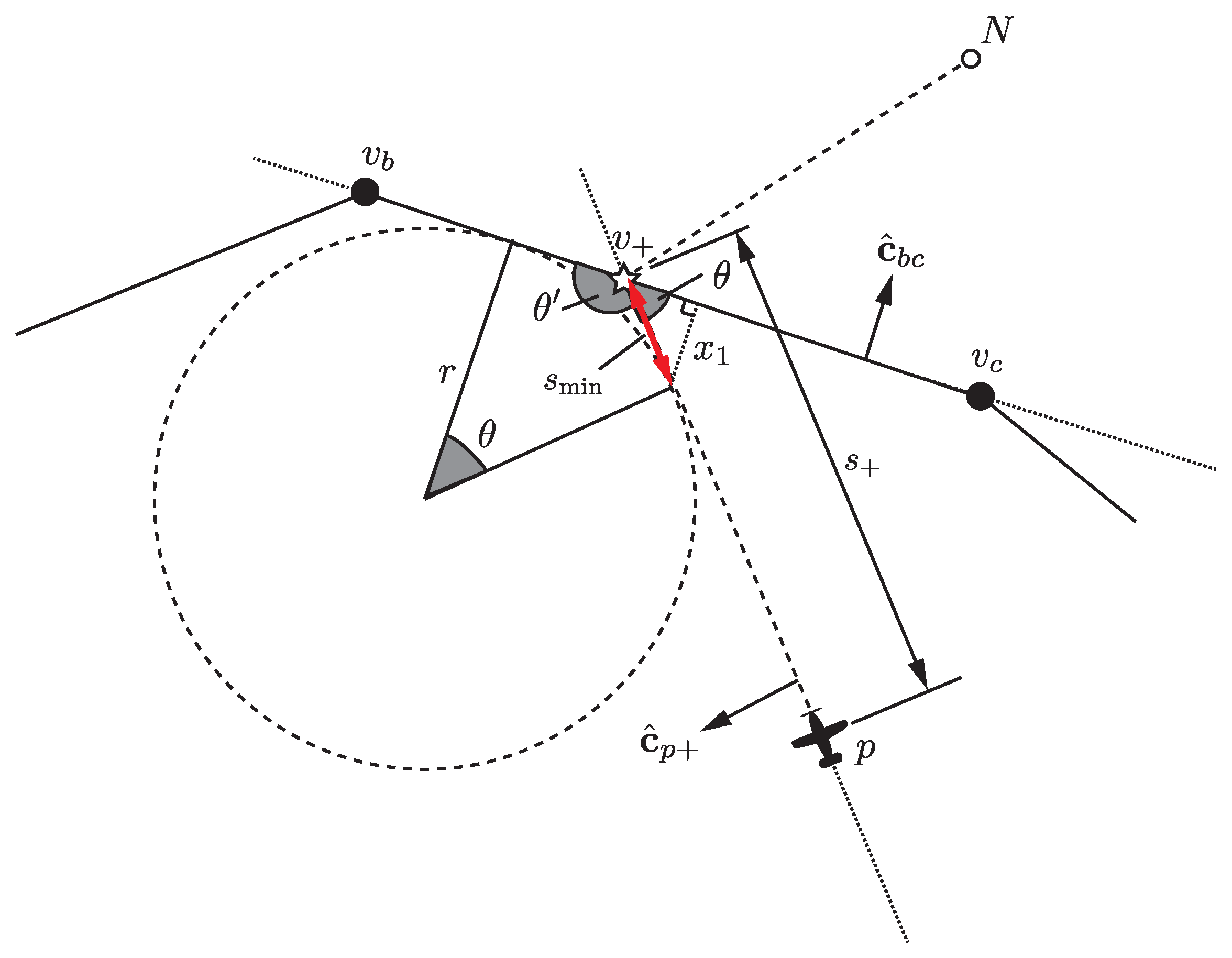
3.2. Calculating Minimum Turn Distance
3.3. Determining the Direction of Turn
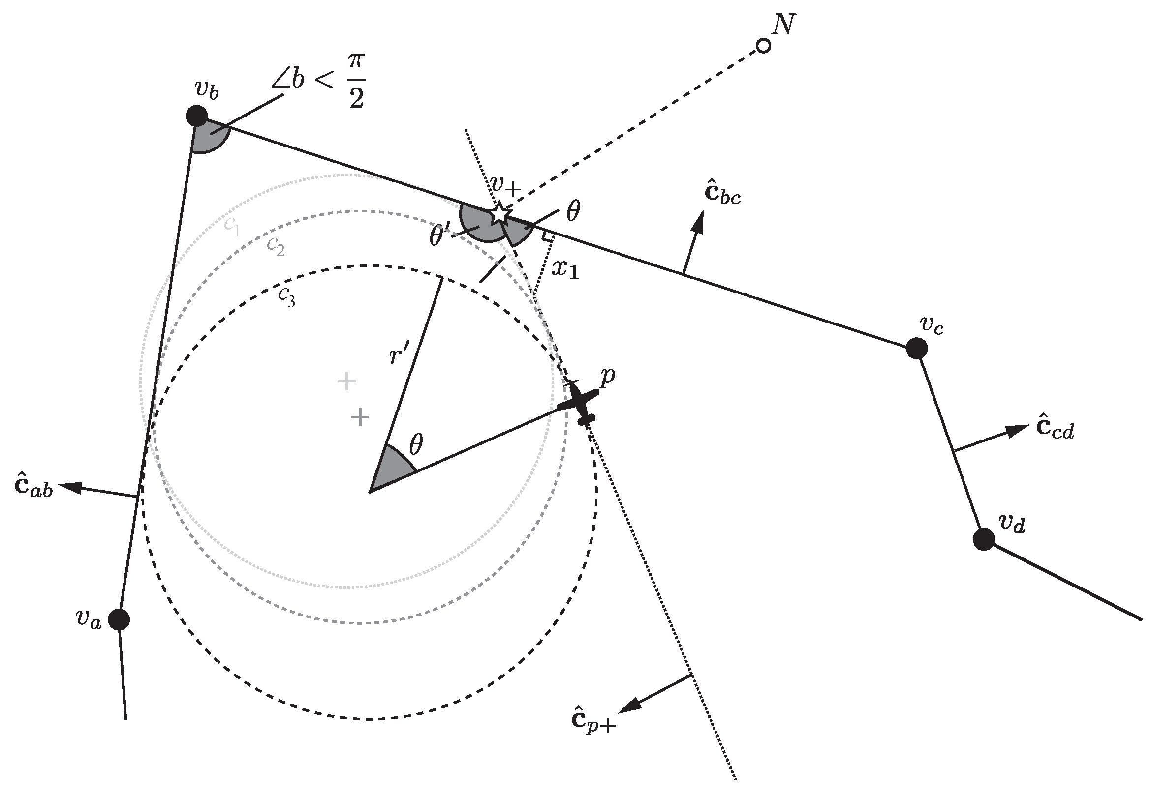
3.4. Acute Internal Angles
3.5. Manual Control
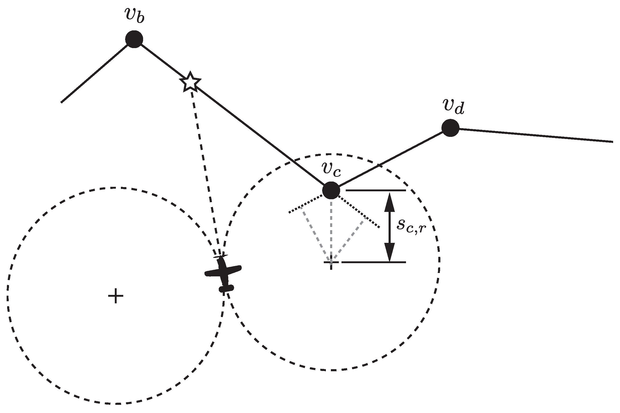
3.6. Excursions
| Algorithm 2 Anticipatory range controller |
| Require: g: Gravitational acceleration
Require: R: Radius of Earth. ▹ or, more generally, R Require: C: Database of n geopost positions for . Require: : N-vector for datum (North). ▹ Require: : User-specified base coordinates. Require: : Maximum bank angle. Require: : Transient effect on turn distance. Require: : Current geodetic coordinates. Require: : Current heading. Require: V: Current speed. ▹ Ideally ground speed Output: |
| Algorithm 3 FENCE: Determine fence intersection |
| Algorithm 4 INTERSECT: Determine intersection of turning circles |
|
| Algorithm 5 TURN: Test the turn criteria |
|
| Algorithm 6 RETURN: Set the anchor point for return |
4. Simulation
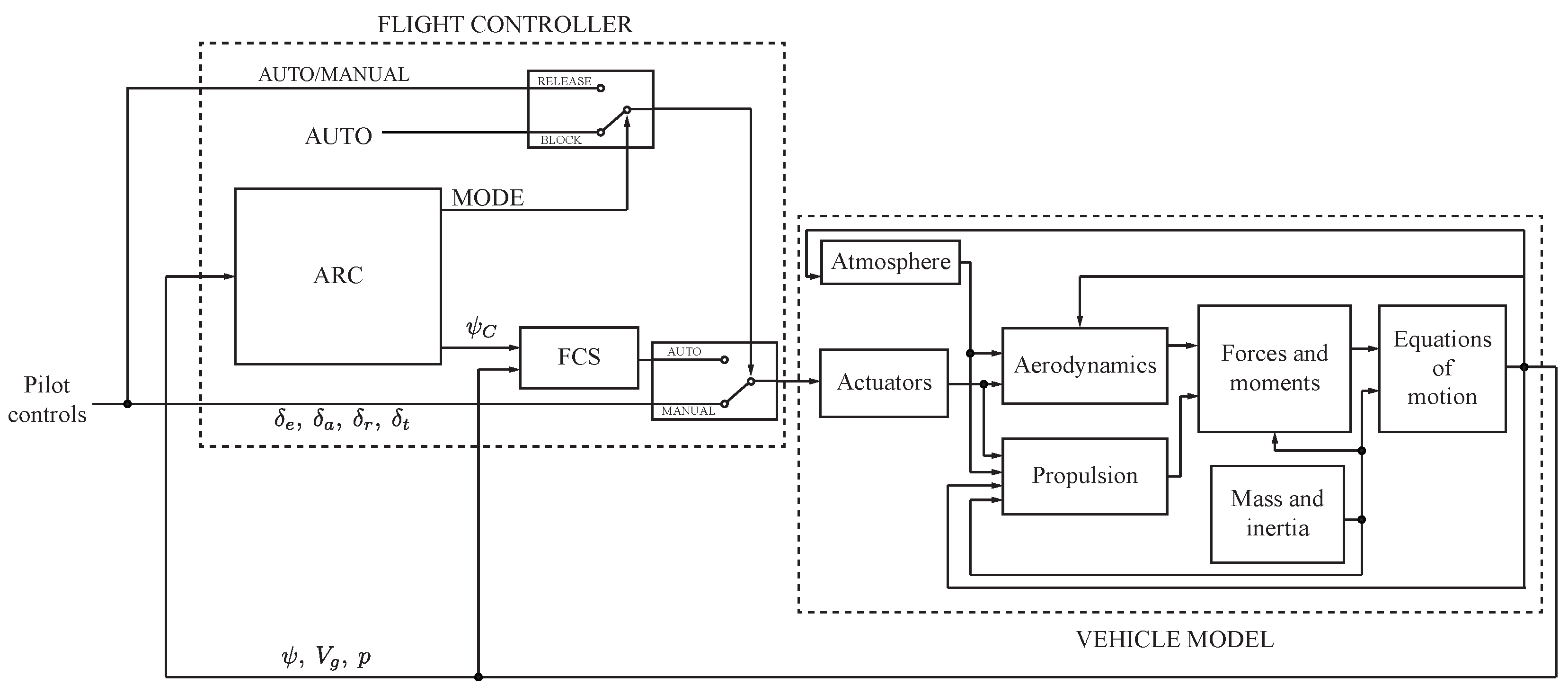
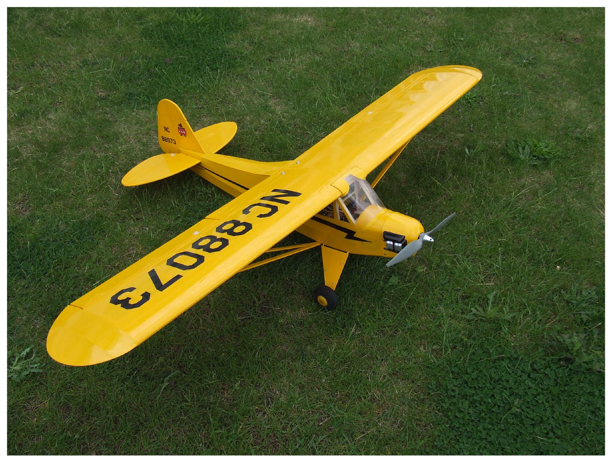
4.1. Vehicle Model
4.2. Geodetic Position
4.3. Vehicle Turn Dynamics
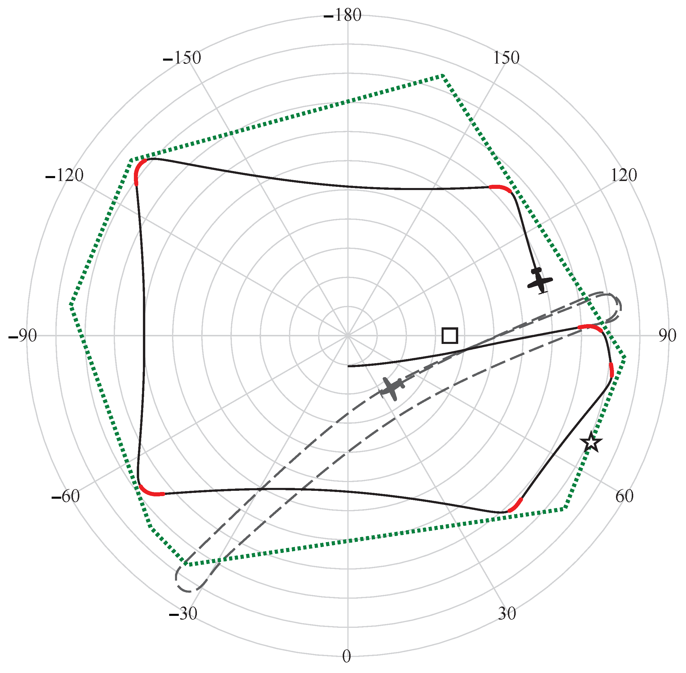
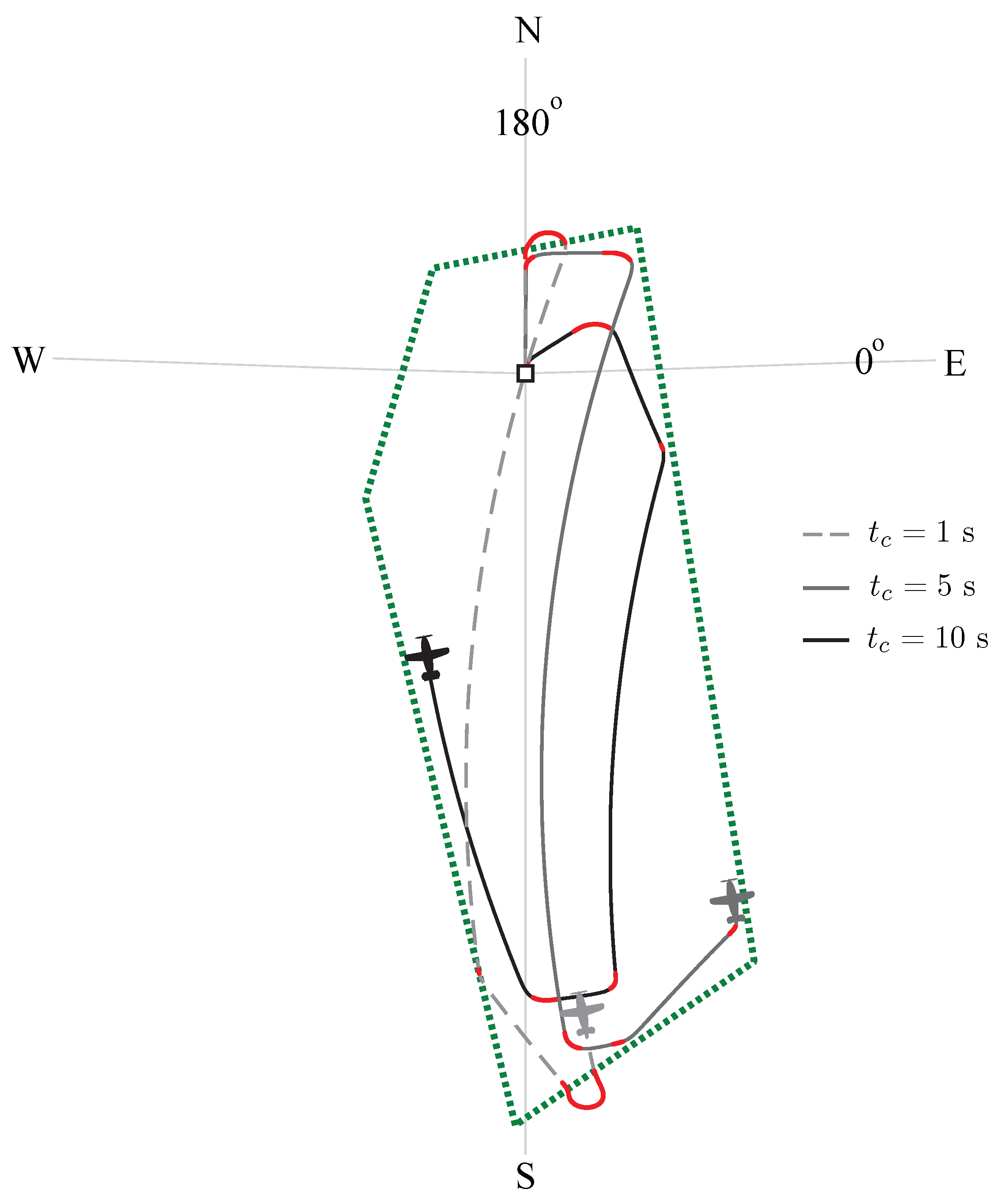
4.4. Simulation Results
5. Remarks
5.1. Algorithm Complexity
5.2. Uncertainty Handling
5.3. Enhancements
5.4. Experimental Validation
6. Conclusions
Author Contributions
Funding
Data Availability Statement
Conflicts of Interest
Nomenclature
| C | Geozone |
| Vector for a plane | |
| g | Acceleration due to gravity |
| h | Altitude |
| Inertia tensor | |
| L | Rolling moment |
| M | Pitching moment |
| m | Mass |
| N | Yawing moment |
| n-vector | |
| n-vector for the intersection point on the geofence | |
| Position vector in ECEF reference frame | |
| p | Position |
| Transformation matrix for angular velocities from ECEF to body axes | |
| Average radius of the Earth | |
| Vertical prime radius curvature of Earth | |
| r | Turn radius |
| s | Distance |
| Minimum distance required to complete a turn | |
| Distance covered to start the turn (i.e., rise-time delay) | |
| Distance to the intersection point with the geofence | |
| t | Time |
| Rise time of the transient roll response | |
| Velocity vector | |
| V | Velocity |
| v | Geopost location |
| w | Winding number |
| X | Axial force |
| Y | Side (or lateral) force |
| Z | Normal force |
| Geometry reference angles | |
| Aileron deflection | |
| Elevator deflection | |
| Rudder deflection | |
| Longitude | |
| Geometric angle | |
| Roll angle | |
| Maximum (commanded) bank angle during a turn | |
| Geodetic latitude | |
| Heading | |
| Heading command | |
| Time constant | |
| Subtended central angle | |
| ℧ | Excursion anchor point |
| Angular velocity vector | |
| AAM | Advanced air mobility |
| ARC | Anticipatory range controller |
| ECEF | Earth-Centered, Earth-Fixed |
| GPS | Global positioning system |
| PID | Proportional-Intergal-Derivative (control) |
| RPV | Remotely piloted vehicle |
| RTB | Return to base |
| UAV | Unmanned air vehicle |
References
- Reclus, F.; Drouard, K. Geofencing for fleet & Freight Management. In Proceedings of the 9th International Conference on Intelligent Transport Systems Telecommunications (ITST), Lille, France, 20–22 October 2009; pp. 353–356. [Google Scholar]
- Stevens, M.N.; Coloe, B.T.; Atkins, E.M. Platform-Independent Geofencing for Low Altitude UAS Operations. In Proceedings of the 15th AIAA Aviation Technology, Integration, and Operations Conference, Dallas, TX, USA, 22–26 June 2015. [Google Scholar]
- Hayhurst, K.J.; Maddalon, J.M.; Neogi, N.A.; Verstynen, H.A. A Case Study for Assured Containment. In Proceedings of the International Conference on Unmanned Aircraft Systems (ICUAS), Denver, CO, USA, 9–12 June 2015; pp. 260–269. [Google Scholar]
- Liu, Y.; Lv, R.; Guan, X.; Zeng, J. Path Planning for Unmanned Aerial Vehicle under Geo-Fencing and Minimum Safe Separation Constraints. In Proceedings of the 12th World Congress on Intelligent Control and Automation (WCICA), Guilin, China, 12–15 June 2016. [Google Scholar]
- Hosseinzadeh, M. UAV geofencing: Navigation of UVAs in constrained environments. In Unmanned Aerial Systems; Elsevier: Amsterdam, The Netherlands, 2021; pp. 567–594. [Google Scholar]
- Lee, H.I.; Shin, H.S.; Tsourdos, A. A Probabilistic–Geometric Approach for UAV Detection and Avoidance Systems. Sensors 2022, 22, 9230. [Google Scholar] [CrossRef] [PubMed]
- Gurriet, T.; Ciarletta, L. Towards a generic and modular geofencing strategy for civilian UAVs. In Proceedings of the International Conference on Unmanned Aircraft Systems (ICUAS), Arlington, VA, USA, 7–10 June 2016; pp. 540–549. [Google Scholar]
- Alarcón, V.; Garcia, M.; Alarcón, F.; Viguria, A.; Martinez, A.; Janisch, D.; Acevedo, J.J.; Maza, I.; Ollero, A. Procedures for the Integration of Drones into the Airspace Based on U-Space Services. Aerospace 2020, 7, 128. [Google Scholar] [CrossRef]
- Nagrare, S.R.; Tony, L.A.; Ratnoo, A.; Ghose, D. Multi-Lane UAV Traffic Management with Path and Intersection Planning. In Proceedings of the AIAA Scitech 2022 Forum, San Diego, CA, USA, 3–7 January 2022. [Google Scholar]
- Kedarisetty, S.; Ratnoo, A. Cooperative Loiter Lane Diversion Guidance Planning for Fixed-Wing UAV Corridors. In Proceedings of the AIAA Scitech 2023 Forum, National Harbor, MD, USA, 23–27 January 2023. [Google Scholar]
- Altun, A.T.; Xu, Y.; Inalhan, G.; Hardt, M.W. Comprehensive Risk Assessment and Utilization for Contingency Management of Future AAM System. In Proceedings of the AIAA Aviation Forum, San Diego, CA, USA, 12–16 June 2023. [Google Scholar]
- Zhang, N.; Liu, H.; Low, K.H. UAV Collision Risk Assessment in Terminal Restricted Area by Heatmap Representation. In Proceedings of the AIAA Scitech 2023 Forum, National Harbor, MD, USA, 23–27 January 2023. [Google Scholar]
- Janson, V.; Ahlbrecht, A.; Durak, U. Architectural Challenges in Developing an AI-based Collision Avoidance System. In Proceedings of the EEE/AIAA 42nd Digital Avionics Systems Conference (DASC), Barcelona, Spain, 1–5 October 2023. [Google Scholar]
- Grüter, B.; Seiferth, D.; Bittner, M.; Holzapfel, F. Emergency Flight Planning using Voronoi Diagrams. In Proceedings of the AIAA SciTech Forum, San Diego, CA, USA, 7–11 January 2019. [Google Scholar]
- Stevens, M.N.; Atkins, E.M. Layered Geofences in Complex Airspace Environments. In Proceedings of the AIAA Aviation Forum, Atlanta, GA, USA, 25–29 June 2018. [Google Scholar]
- Zhang, S.; Wei, D.; Huynh, M.Q.; Quek, J.X.; Ma, X.; Xie, L. Model Predictive Control Based Dynamic Geofence System for Unmanned Aerial Vehicles. In Proceedings of the AIAA Information Systems-AIAA Infotech @ Aerospace, Grapevine, TX, USA, 9–13 January 2017. [Google Scholar]
- Cavanini, L.; Ferracuti, F.; Ippoliti, G.; Orlando, G. Model Predictive Control for UAV Geofencing. In Proceedings of the 9th International Conference on Control, Decision and Information Technologies, Rome, Italy, 3–6 July 2023. [Google Scholar]
- Seiferth, D.; Gruter, B.; Heller, M.; Holzapfel, F. Fully-Automatic Geofencing Module for Unmanned Air Systems In Two Dimensional Space. In Proceedings of the AIAA Scitech 2019 Forum, San Diego, CA, USA, 7–11 January 2019. [Google Scholar]
- Theile, M.; Yu, S.; Dankster, O.D.; Caccamo, M. Trajectory estimation for geo-fencing applications on small-size fixed-wing UAVs. In Proceedings of the 2019 IEEE/RSJ International Conference on Intelligent Robots and Systems (IROS), Macau, China, 3–8 November 2019. [Google Scholar]
- Stevens, M.N.; Atkins, E.M. Multi-Mode Guidance for an Independent Multicopter Geofencing System. In Proceedings of the 16th AIAA Aviation Technology, Integration, and Operations Conference, Washington, DC, USA, 12–16 July 2016. [Google Scholar]
- Dill, E.T.; Young, S.D.; Hayhurst, K.J. SAFEGUARD: An assured safety net technology for UAS. In Proceedings of the 2016 IEEE/AIAA 35th Digital Avionics Systems Conference (DASC), Sacramento, CA, USA, 25–29 September 2016. [Google Scholar]
- D’Souza, S.; Ishihara, A.; Nikaido, B. Feasibility of Varying Geo-Fence around an Unmanned Aircraft Operation based on Vehicle Performance and Wind. In Proceedings of the 2016 IEEE/AIAA 35th Digital Avionics Systems Conference (DASC), Sacramento, CA, USA, 25–29 September 2016. [Google Scholar]
- Stevens, M.N.; Atkins, E.M. Generating Airspace Geofence Boundary Layers in Wind. J. Aerosp. Inf. Syst. 2019, 17, 113–124. [Google Scholar] [CrossRef]
- Seiferth, D.; Holzapfel, F.; Heller, M. Evasive Maneuvers of Optionally Piloted Air Vehicles For Three-Dimensional Geofencing. In Proceedings of the AIAA Scitech 2020 Forum, Orlando, FL, USA, 6–10 January 2020. [Google Scholar]
- Ghaffari, A. Analytical Design and Experimental Verification of Geofencing Control for Aerial Applications. IEEE/ASME Trans. Mechatron. 2021, 26, 1106–1117. [Google Scholar] [CrossRef]
- Vagal, V.; Markantonakis, K.; Shepherd, C. A New Approach to Complex Dynamic Geofencing for Unmanned Aerial Vehicles. In Proceedings of the IEEE/AIAA 40th Digital Avionics Systems Conference (DASC), San Antonio, TX, USA, 3–7 October 2021; pp. 1–7. [Google Scholar]
- Kim, J.; Mathur, A.; Liberko, N.; Atkins, E. Operational Volumization and Inverse Volumization for Low-Altitude Airspace Geofencing. In Proceedings of the AIAA Aviation Forum, Virtual Event, 2–6 August 2021. [Google Scholar]
- Kim, J.; Atkins, E. Airspace Geofencing and Flight Planning for Low-Altitude, Urban, Small Unmanned Aircraft Systems. Appl. Sci. 2022, 12, 576. [Google Scholar] [CrossRef]
- Bhise, A.A.; Garg, S.; Ratnoo, A.; Ghose, D. Signed Distance Function based Geofencing for UAV Corridors. In Proceedings of the AIAA Scitech Forum, Virtual, San Diego, CA, USA, 3–7 January 2022. [Google Scholar]
- Nagrare, S.R.; Ratnoo, A.; Ghose, D. Multi-intersection planning with durational speed scheduling for drone corridors. In Proceedings of the AIAA Scitech 2023 Forum, National Harbor, MD, USA, 23–27 January 2023. [Google Scholar]
- Haines, E. Point in Polygon Strategies. In Graphics Gems IV; Heckbert, P.S., Ed.; Academic Press: Cambridge, MA, USA, 1994; pp. 24–46. [Google Scholar]
- Shimrat, M. Algorithm 112: Position of point relative to polygon. Commun. ACM 1962, 5, 434. [Google Scholar] [CrossRef]
- Hacker, R. Certification of Algorithm 112: Position of point relative to polygon. Commun. ACM 1962, 5, 606. [Google Scholar] [CrossRef]
- Hormann, K.; Agathos, A. The point in polygon problem for arbitrary polygons. Comput. Geom. 2001, 20, 131–144. [Google Scholar] [CrossRef]
- Alciatore, D.G.; Miranda, R. A Winding Number and Point-In-Polygon Algorithm; Colorado State University: Fort Collins, CO, USA, 1995. [Google Scholar]
- Sutherland, I.E.; Sproull, R.F.; Schumacker, R.A. A Characterization of Ten Hidden-Surface Algorithms. ACM Comput. Surv. 1974, 6, 1–55. [Google Scholar] [CrossRef]
- Gatilov, S. Efficient Angle Summation Algorithm for Point Inclusion Test and Its Robustness. Reliab. Comput. 2013, 19, 1–25. [Google Scholar]
- Badouel, D. An Efficient Ray-Polygon Intersection. In Graphics Gems; Glassner, A.S., Ed.; Academic Press: Cambridge, MA, USA, 1990; pp. 390–393. [Google Scholar]
- Fieto, F.R.; Torres, J.C. Inclusion Test for General Polyhedra. Comput. Graph. 1997, 21, 23–30. [Google Scholar] [CrossRef]
- Moeller, T.; Trumbore, B. Fast, minimum storage ray triangle intersection. J. Graph. Tools 1997, 2, 21–28. [Google Scholar] [CrossRef]
- Dobkin, D.; Guibas, L.; Hershberger, J.; Snoeyink, J. An efficient algorithm for finding the CSG representation of a simple polygon. In Proceedings of the 15th Annual Conference on Computer Graphics and Interactive Techniques, New York, NY, USA, 1–5 August 1988; Dill, J., Ed.; ACM Press: New York, NY, USA, 1988; Volume 22, pp. 31–40. [Google Scholar]
- Walker, R.J.; Snoeyink, J. Practical point-in-polygon tests using CSG representations of polygons. In Proceedings of the Algorithm Engineering and Experimentation Meeting, Baltimore, MD, USA, 15–16 January 1999; Goodrich, M.T., McGeoch, C.C., Eds.; Springer: Berlin/Heidelberg, Germany, 1999; Volume 1619, pp. 114–128. [Google Scholar]
- Preparata, F.P.; Shamos, M.I. Computational Geometry: An Introduction; Springer: New Your, NY, USA, 1985; pp. 41–67. [Google Scholar]
- Bentley, J.L. Algorithms for Reporting and Counting Geometric Intersections. IEEE Trans. Comput. 1979, C-28, 643–647. [Google Scholar] [CrossRef]
- Prasad, M. Intersection of line segments. In Graphics Gems II; Arvo, J., Ed.; Academic Press: Cambridge, MA, USA, 1991; pp. 7–9. [Google Scholar]
- Antonio, F. Faster Line Segment Intersection. In Graphics Gems III; Kirk, D., Ed.; Academic Press: Cambridge, MA, USA, 1991; pp. 199–202. [Google Scholar]
- Pratyusha, P.L.; Naidu, V.P.S. Geo-Fencing for Unmanned Aerial Vehicle. In Proceedings of the National Conference “Electronics, Signals, Communication and Optimization” (NCESCO), Mysuru, Karnataka, 9 September 2015; pp. 1–7. [Google Scholar]
- Thomas, P.R.; Richardson, T.S.; Cooke, A.K. Estimation of Stability and Control Derivatives for a Piper Cub J-3 Remotely Piloted Vehicle. In Proceedings of the AIAA Modeling and Simulation Technologies Conference, Minneapolis, MN, USA, 13–16 August 2012; pp. 1–26. [Google Scholar]
- Bowring, B.R. Transformation from spatial to geographical coordinates. Surv. Rev. 1976, 23, 323–327. [Google Scholar] [CrossRef]
- Watson, A.H.; McCabe, T.J. Structured Testing: A Testing Methodology Using the Cyclomatic Complexity Metric; NIST Special Publication 500-235; National Institute of Standards and Technology: Gaithersburg, MD, USA, 1996.
- Gros, S.; Quirynen, R.; Diehl, M. Aircraft control based on fast non-linear MPC & multiple-shooting. In Proceedings of the 51st IEEE Conference on Decision and Control (CDC), Maui, HI, USA, 10–13 December 2012. [Google Scholar]
- Stastny, T.; Dash, A.; Siegwart, R. Nonlinear MPC for Fixed-wing UAV Trajectory Tracking: Implementation and Flight Experiments. In Proceedings of the AIAA Scitech Forum, Grapevine, TX, USA, 9–13 January 2017. [Google Scholar]
- Zhu, G.; Wei, P. Low-Altitude UAS Traffic Coordination with Dynamic Geofencing. In Proceedings of the 16th AIAA Aviation Technology, Integration, and Operations Conference, Washinton, DC, USA, 13–17 June 2016. [Google Scholar]
- Kuenz, A.; Lieb, J.; Rudolph, M.; Volkert, A.; Geister, D.; Ammann, N.; Zhukov, D.; Feurich, P.; Gonschorek, J.; Gessner, M.; et al. Live Trials of Dynamic Geo-Fencing for the Tactical Avoidance of Hazard Areas. IEEE Aerosp. Electron. Syst. Mag. 2023, 38, 60–71. [Google Scholar] [CrossRef]
- Ardupilot Project. Available online: https://ardupilot.org (accessed on 1 June 2023).
- Oborne, M. Mission Planner, v1.3.81. Available online: https://ardupilot.org/planner/ (accessed on 1 June 2023).


| Symbol | Description |
|---|---|
| X, Y, Z | Forces in the axial, lateral, and normal directions, respectfully. |
| L, M, N | Moments about the x, y, and z axes, respectfully. |
| m | Aircraft’s mass |
| Aircraft’s inertia tensor. | |
| Velocity vector in the body reference frame, . | |
| Position vector in the ECEF reference frame, . | |
| Angular velocity vector in the body reference frame, . | |
| Transformation matrix to transform angular velocities from ECEF to body reference frame. |
| # | Algorithm | Cyclomatic Complexity |
|---|---|---|
| Algorithm 1 | Return to base | 2 |
| Algorithm 2 | ARC | 37 |
| Algorithm 3 | → FENCE | → 7 |
| Algorithm 4 | → INTERSECT | → 16 |
| Algorithm 5 | → TURN | → 8 |
| Algorithm 6 | → RETURN | → 5 |
Disclaimer/Publisher’s Note: The statements, opinions and data contained in all publications are solely those of the individual author(s) and contributor(s) and not of MDPI and/or the editor(s). MDPI and/or the editor(s) disclaim responsibility for any injury to people or property resulting from any ideas, methods, instructions or products referred to in the content. |
© 2024 by the authors. Licensee MDPI, Basel, Switzerland. This article is an open access article distributed under the terms and conditions of the Creative Commons Attribution (CC BY) license (https://creativecommons.org/licenses/by/4.0/).
Share and Cite
Thomas, P.R.; Sarhadi, P. Geofencing Motion Planning for Unmanned Aerial Vehicles Using an Anticipatory Range Control Algorithm. Machines 2024, 12, 36. https://doi.org/10.3390/machines12010036
Thomas PR, Sarhadi P. Geofencing Motion Planning for Unmanned Aerial Vehicles Using an Anticipatory Range Control Algorithm. Machines. 2024; 12(1):36. https://doi.org/10.3390/machines12010036
Chicago/Turabian StyleThomas, Peter R., and Pouria Sarhadi. 2024. "Geofencing Motion Planning for Unmanned Aerial Vehicles Using an Anticipatory Range Control Algorithm" Machines 12, no. 1: 36. https://doi.org/10.3390/machines12010036
APA StyleThomas, P. R., & Sarhadi, P. (2024). Geofencing Motion Planning for Unmanned Aerial Vehicles Using an Anticipatory Range Control Algorithm. Machines, 12(1), 36. https://doi.org/10.3390/machines12010036