Accurate Recognition Method for Rolling Bearing Failure of Mine Hoist in Strong Noise Environment

Abstract

The operating environment of rolling bearings in mine hoists is complicated, and detecting their faults is hindered by a weak and unstable initial vibration signal. This directly affects the ability to extract pertinent fault features. This paper puts forward an adaptive fault diagnosis method for rolling bearings that combines the Variational Modal Decomposition (VMD) model and Vision Transformer (ViT) deep learning network model. The objective was to address the difficulty of extracting relevant fault features from bearing vibration signals in environments with strong noise levels. First, an improved VMD+ViT model was used to remove the strong noise from the original bearing signal and adaptively classify the fault types; then, the impacts of modal components and encoder numbers on the accuracy of fault diagnosis were explored. Finally, the proposed methodology was validated by applying it to actual rolling bearing fault data, including both open-source and fault test datasets. The research findings indicated that employing a VMD+ViT integrated model consisting of one modal component with the highest Pearson correlation coefficient and eight encoders resulted in high accuracy in diagnosing faults, even in the presence of high levels of noise in the bearing’s vibration signal. The proposed diagnostic method achieved a diagnostic accuracy of over 92.70% on the open-source bearing dataset with strong interference noise and over 98.62% on the fault test dataset. The proposed method exhibited high accuracy and strong robustness, making it suitable for effectively diagnosing and accurately identifying different categories of rolling bearing faults in mine hoists, even in environments with high levels of noise.

1. Introduction

Mineral resources have an important position in modern construction and heavy industry development. The mine hoist is the main equipment for mineral resource mining, and its safe operation is crucial. Rolling bearings are the key parts of the mine hoist. In the mine environment, environmental conditions such as temperature and humidity affect the operating condition of the bearings, increasing the probability of bearing failure generation. In addition, the working state of the mine hoist itself, the surrounding environment, and the signals generated by other equipment will produce strong noise. This interference noise will confuse the signals generated by bearing faults, which makes the timely diagnosis of bearing faults difficult and may cause fault omission or misdiagnosis, affecting the accuracy of diagnosis.

In bearing fault detection, the fault signal incorporates a significant amount of operational state information, and it is the objective of researchers to mine potential fault information from this complex signal. However, since the fault signal is commonly nonlinear and nonstationary, the weak characteristic signal of the bearing fault can become overwhelmed by robust background noise elements such as alternating current and fundamental frequency harmonics [1]. In the strong noise background, the fault impact feature information of the bearing vibration signal is weak, necessitating high requirements for fault detection methods, and it is necessary to accurately determine the operation status of the bearing and discover the operation fault as soon as possible. Therefore, the realization of feature extraction of bearings in strong noise environments is a complex and urgent problem for domestic and foreign research and of great significance to ensure the healthy operation of machines.

In recent years, researchers have proposed leveraging time–frequency domain analysis methods to address signal processing challenges posed by strong noise environments. Notable methods include the Short-Time Fourier Transform (STFT) [2], Wavelet Transform (WT) [3], and Empirical Mode Decomposition (EMD) [4], among others. Zhou et al. [5] utilized the STFT approach to process vibration signals, constructing the signal’s time–frequency map. This move circumvented information loss in fault characteristics while ensuring the effective and practical representation of the vibration signal’s fault features. Yi et al. [6] relied upon the STFT method to formulate the de-noise STFT, exploiting the sparsity property of the time–frequency domain’s transform coefficient and the non-convex penalized low-rank matrix with adaptive decomposition. This effectively eliminated the influence of randomly distributed noise in the time–frequency map. Baojia et al. [7] combined multi-scale wavelet decomposition, wavelet analysis local optimization, and multi-resolution features to reconstruct the signal’s low-resonance components. This approach effectively extracted characteristic fault information from the bearing failure signal, solving the challenge of strong background noise seriously undermining the early fault diagnosis of rolling bearings. Pl et al. [8] utilized the Wavelet Transform (WT) time–frequency domain conversion capability along with signal de-noising techniques to convert the one-dimensional vibration signal in the time domain sequence data collected from rolling bearings into two-dimensional time–frequency domain images. These temporal frequency images were used as input to a deep learning model in order to extract and classify fault features with high diagnostic accuracy, especially in the presence of strong background noise. Meng et al. [9] applied Empirical Mode Decomposition (EMD) to extract the vibration signal characteristics of rolling bearings and obtain the corresponding eigenmodal functions. Then, they filtered the characteristic information using a designed kurtosis criterion to identify the correspondence between the actual and theoretically calculated values of the fault frequency, aiming to achieve precise fault analysis.

Variational Mode Decomposition (VMD) is an adaptive and non-recursive approach to modal variation and signal processing. This technique offers several advantages, including the ability to self-determine the number of modal decompositions, high complexity reduction, and the capacity to handle strong non-linearities and time series non-smoothness. Chi et al. [10] employed an efficient and robust variable scale non-recursive signal processing method based on the VMD method to extract characteristic information from non-stationary signals while ignoring end effects. Meanwhile, Li et al. [11] proposed a criterion for determining the number of decompositions, K, by calculating the difference between the center frequencies of each eigenmodal function following decomposition. Wu et al. [12] utilized the VMD algorithm to decompose vibration signals into multiple modal components. Next, they introduced the Kernel Joint Approximate Diagonalized Eigenmatrix (KJADE) to reduce the dimensionality of the high-dimensional eigenmatrix, allowing for efficient preprocessing of data in the fault diagnosis process. Liu et al. [13] employed the VMD method to perform orthogonal decomposition of the vibration signal, resulting in a reflection of the distribution characteristics across different frequency bands of the original signal. This approach allowed for highly accurate diagnosis of rolling bearing faults.

The signal-to-noise separation algorithm of VMD can overcome the limitations of traditional signal-to-noise separation algorithms and effectively eliminate the influence of noise in the original signal from the mine hoist’s main bearing. By combining the reconstructed de-noised vibration signals with advanced fault diagnosis methods, accurate identification and classification of main bearing faults can be achieved.

In comparison to traditional methods for bearing fault diagnosis, deep learning-based approaches for rolling bearing fault diagnosis offer the ability to automatically select and extract features from data, resulting in a significant improvement in the accuracy and adaptability of fault identification algorithms [14]. Common deep learning models for bearing fault diagnosis include Convolutional Neural Network (CNN), Deep Belief Network (DBN), Recurrent Neural Network (RNN), Vision Transformer (ViT), and other network models. Shuuji et al. [15], for example, utilized an improved statistical filtering algorithm to extract fault signals from a factory noise background. They then used a CNN to automatically extract the signal features and create a fault classification model for diagnosing low-speed bearing signals. Zhang et al. [16] input the bearing vibration features adaptively extracted by a one-dimensional CNN into a support vector machine, thereby improving the classification accuracy of bearing faults. Gao et al. [17] developed a new optimal adaptive Deep Belief Network (DBN) model with a stochastic gradient descent using a minimum batch size to enhance the accuracy of fault identification classification. Li et al. [18] developed a two-stage attentional recurrent neural network (DA-RNN), which was designed to enhance the accuracy and stability of fault diagnosis models for unbalanced datasets under practical working conditions.

The ViT network model is a powerful deep learning architecture that captures global information more effectively in images. In contrast to the CNN model, which requires retraining for images of different sizes, ViT can segment the image and learn the interrelationship of the small pieces in the image through a multilayer self-attentive mechanism, thus better capturing the global information of the image. Additionally, the ViT model has the capability to automatically select and extract features from large amounts of data, which greatly improves the accuracy and adaptability of fault recognition algorithms [19]. Dosovitskiy et al. [20] argued that combining attentional mechanisms with CNNs was unnecessary in visual processing and proposed the Vision Transformer (ViT) model. Although ViT networks lack the inductive bias of CNN networks, the results can be competitive with state-of-the-art CNN networks. Sharma et al. [21] proposed a method called Locally Aware Transformer (LAT), which built on the ViT model. The LAT method added the global features of ViT directly to each block of local features, disregarding the correlation between local features. The information between local and global features was then fused to improve target recognition accuracy. Touvron et al. [22] addressed the challenge of ViT relying on large amounts of training data by introducing a distillation mechanism to train ViT networks. This approach improved the classification efficiency of ViT, making it possible to train a more effective model with less data. Han et al. [23] discussed the challenges encountered by different visual class Transformer models in various classification tasks and compared their performance. ViT has demonstrated excellent performance in Fine-Grained Visual Recognition (FGVR). Additionally in this field, Zhang et al. [24] proposed the adaptive attention multiscale fusion Transformer method to compensate for ViT’s limitations and capture regional attention. This method enhanced ViT’s FGVR performance.

In conclusion, this paper puts forward a new approach that combines VMD and ViT to improve the diagnostic accuracy in identifying bearing faults even in the presence of strong noise. This method was applied to analyze the vibration signals measured from a rolling bearing test rig, and it can play a crucial role in precisely detecting and classifying the main bearing fault categories in mine hoists. The proposed approach will be particularly useful in complex and challenging environments.

2. Characteristics of Rolling Bearing Failure Diagnosis Method

2.1. The Process of Fault Diagnosis Method Combining VMD and ViT

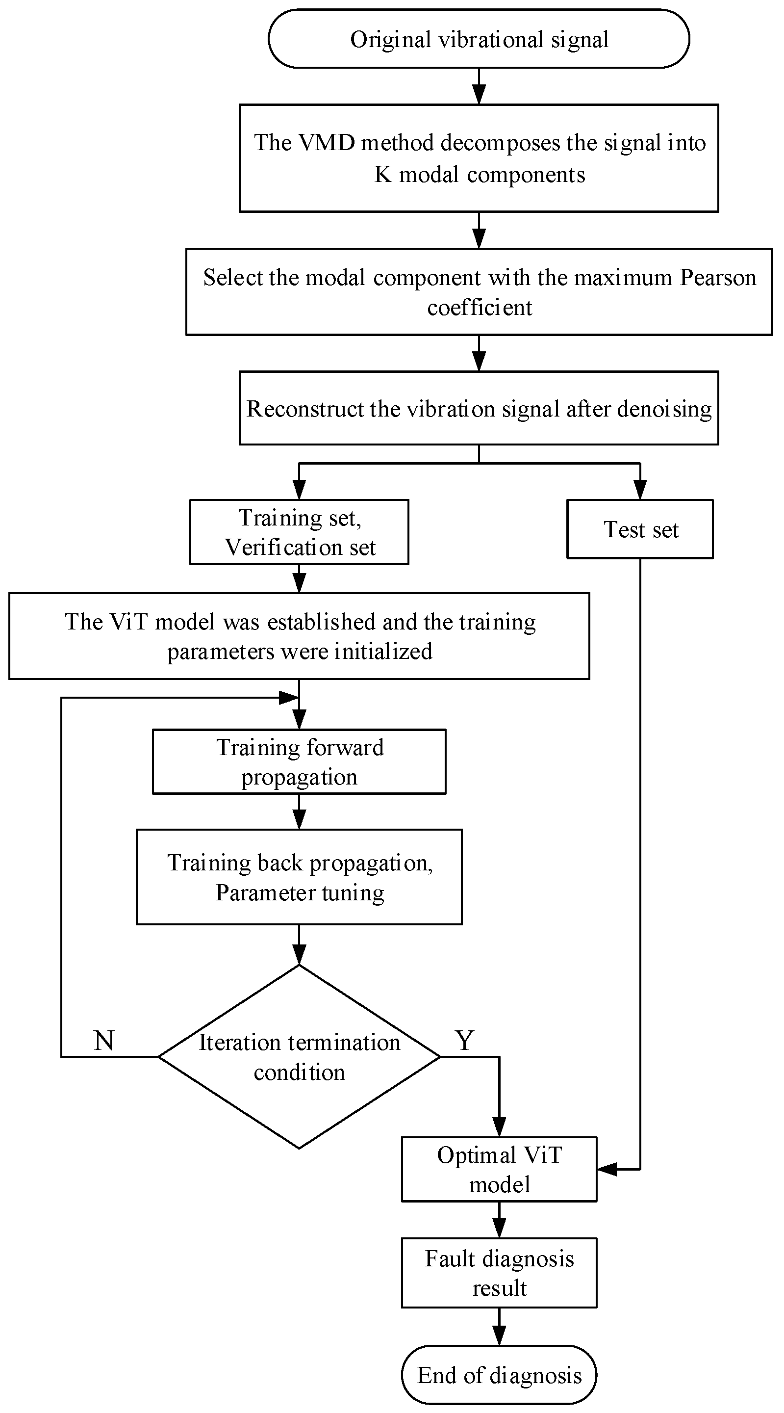
This paper proposes a fault diagnosis approach for the main bearing of a mine hoist using a combination of VMD and ViT. Initially, the VMD algorithm is employed to implement signal decomposition and reconstruction. Subsequently, a fast Fourier transform is applied to obtain the spectrum map of the de-noised reconstructed signal. The signal spectrum image is then fed into the ViT network for feature extraction, and the classifier is trained to diagnose the fault categories based on the extracted features. The proposed method’s flow diagram is presented in Figure 1.

2.2. Research on VMD Signal Pre-Processing Algorithm

The VMD algorithm works by finding a set of modes and their respective center frequencies so that these modes can work together to smoothly reproduce the input signal. The essence of the algorithm is to extend the classical Wiener filter to multiple adaptive frequency bands. To efficiently optimize the variational model, the alternating direction multiplier method is employed, rendering the model robust to sampling noise.

Assume that the real-valued signal, f, can be decomposed into K sparse eigenmodal components, $u_k$, and the spectrum of each component is concentrated in a certain bandwidth, with ${\omega }_k$ as the center frequency. The objective of VMD decomposition is to minimize the bandwidth of each component while satisfying the sparsity condition, i.e., the mode components are required to be concentrated around their central frequency, ${\omega }_k$. To this end, the Hilbert transform of a set of modal components, $u_k$, is used to obtain the analytic signal, $u_{A,}{}_k$. The modulation method is used to translate the analytic signal and establish the optimal objective function based on the gradient 2nd order parametric equation, as follows [25]:

$$\underset{\left\{u_k\right\},\left\{{\omega }_k\right\}}{\min }\left\{{\displaystyle \sum _k{\Vert {\partial }_t\left[\left(\delta \left(t\right)+\frac{j}{\pi t}\right)\ast u_k\left(t\right)\right]e^{-j{\omega }_{k}t}\Vert }_2^2}\right\}$$

(1)

$$such that{\displaystyle \sum _k{u}_k=f}$$

(2)

In the formula, $\left\{uk\right\}=\left\{u1,u2,\dots ,uk\right\}$ is K modal components; $\left\{\omega k\right\}=\left\{\omega 1,\omega 2,\dots ,\omega k\right\}$ is the central frequency of each component; $f$ is the input signal; $\ast$ is the sign of the convolution operation; and $\partial t$ is the sign of the gradient operation.

The constrained optimization problem of Formulas (1) and (2) is converted into an unconstrained problem by introducing the quadratic penalty term, α, and the Lagrange multiplicative operator, $\lambda \left(t\right)$, with the augmented Lagrangian function as:

$$\begin{array}{c}L\left(\left\{u_k\right\},\left\{{\omega }_k\right\},\lambda \right)=\alpha {\displaystyle \sum _k{\Vert {\partial }_t\left[\left(\delta \left(t\right)+\frac{j}{\pi t}\right)\ast u_k\left(t\right)\right]e^{-j{\omega }_{k}t}\Vert }_2^2}\\ +{\Vert f\left(t\right)-{\displaystyle \sum _k{u}_k\left(t\right)}\Vert }_2^2+\langle \lambda (t),f\left(t\right)-{\displaystyle \sum _k{u}_k\left(t\right)}\rangle \end{array}$$

(3)

In the formula, $\alpha$ is the penalty factor; $\lambda \left(t\right)$ is the Lagrange multiplier operator; and $\langle \rangle$ is the inner product operation.

After establishing the unconstrained optimization objective function, the Alternating Direction Method of Multipliers (ADMM) is used to iteratively find the optimum for each modal component. First, a set of $u_k$ is assumed as a general condition, and the central frequency, ${\omega }_k$, that minimizes Formula (3) is calculated. Then, the new central frequency, ${\omega }_k$, is taken as a general condition and the $u_k$ that minimizes Formula (3) is calculated. In this way, $u_k$ and ${\omega }_k$ are alternately updated until the algorithm converges or terminates; that is, the optimum values of $u_k$ and ${\omega }_k$ are determined, and the VMD decomposition process is complete.

The VMD algorithm can adaptively decompose a complex signal into multiple effective AM-FM signal combinations by frequency domain iterations. It can decompose a non-smooth input signal, $Y$, into K modal components with specific sparsity. In the decomposition process, if the selected K value is too large, it will lead to over-decomposition, and one that is too small will lead to under-decomposition. To avoid over- and under-decomposition, this paper used the Pearson correlation coefficient to calculate the correlation degree between the decomposed signal components and the original signal to determine the K value [26]. The Pearson coefficient, $\gamma \left(X,Y\right)$, can be expressed as:

$$\gamma \left(X,Y\right)=\mathrm{Cov}(X,Y)/(\sigma X\cdot \sigma Y)$$

(4)

In the formula, $X$ and $Y$ are two random variables, $Cov\left(X,Y\right)$ denotes the covariance of $X$ and $Y$; and $\sigma X$ and $\sigma Y$ indicate the standard deviation of X and Y, respectively.

The K value was determined by the following procedure:

(1)

Set the initial number of modal components K = 2, (K ≤ 10);

(2)

Decomposition of vibration signals by VMD;

(3)

Determine $\gamma (u_{k-1},f)\ge \gamma (u_k,f)$, and if it indicates that the VMD over-decomposes so that K = K − 1, the loop ends; otherwise, let K = K + 1 and re-iterate step (2).

The initial value of K was set to 2. The correlation coefficients obtained for each modal component are listed in

Table 1. Correlation coefficient of Κ value corresponding to each modal component.

K	IMF1	IMF2	IMF3	IMF4	IMF5
2	0.4645	0.5329	—	—	—
3	0.4450	0.4533	0.5070	—	—
4	0.4219	0.4293	0.4255	0.4880	—
5	0.3734	0.4185	0.4368	0.4966	0.4148

.

Table 1 illustrates that for K values of 2, 3, and 4, the Pearson correlation coefficient corresponding to the IMF produced by the last decomposition was greater than the Pearson coefficient produced by the penultimate decomposition. When K equaled 5, IMF4 was greater than IMF5. The principal reason for this disparity was the over-decomposition of the signal during the signal decomposition process. Similarly, when K was equal to 2 and 3, the signal was not fully decomposed in the decomposition process. Hence, for the above-simulated signal, the modal component IMF4 with the most significant Pearson coefficient was selected as the optimal number of intrinsic mode functions (IMFs) to effectively reconstruct the useful signal. Sensitivity analysis was conducted by varying the number of modal components, K, to assess its impact on the signal de-noising performance. Comparisons between the signal frequency spectrum of the original noise-added analog signal and the reconstructed signal post-VMD decomposition showed that the VMD method had the potential to substantially weaken the noise components in the reconstructed signal and accentuate the fault information, blending with the optimal K values.

Once the modal number K is established, each modal component is obtained via VMD decomposition, and the Pearson correlation coefficient between each mode and the original signal is determined. The modal components are then arranged based on the magnitude of their correlation coefficients. Finally, the valid signal is reconstructed by assembling the components accordingly. Figure 2 displays the de-noising effect of the bearing fault signal.

To simulate rolling bearing fault data under strong background noise, a synthetic signal was generated by adding a robust background noise component to the original fault impulse signal (as shown in Figure 2c). After adding the noise component, the time domain signal became crowded, the original fault impulse signal’s frequency features were overwhelmed by the noise component, and the characteristic fault frequencies could not be effectively separated (as shown in Figure 2d). The VMD signal-to-noise separation algorithm was utilized to process the fault signal to extract the original vibration signal from the noise-added signal. After undergoing processing via the VMD algorithm, the noise-added time domain waveform resembled the original waveform structure (as shown in Figure 2e). The noise component in the reconstructed signal spectrum was reduced and the frequency characteristics were apparent (as shown in Figure 2f).

Combined with the whole of Figure 2, it could be seen that VMD, as an adaptive signal separation method, decomposed the signal into multiple eigenmodal components and selected the signal components with less noise information in the modal components and the greatest correlation with the original signal for combination. Additionally, the noise interference of the signal after recombination was significantly reduced, and the key information was retained. Furthermore, some components in the time domain signal may have cancelled each other in the time axis and could not be observed, but they could be clearly seen in the frequency domain. Therefore, the FFT analysis of the noise-reduced signal after VMD decomposition and reconstruction could accurately obtain the frequency domain information of the signal.

2.3. ViT Network Model Building

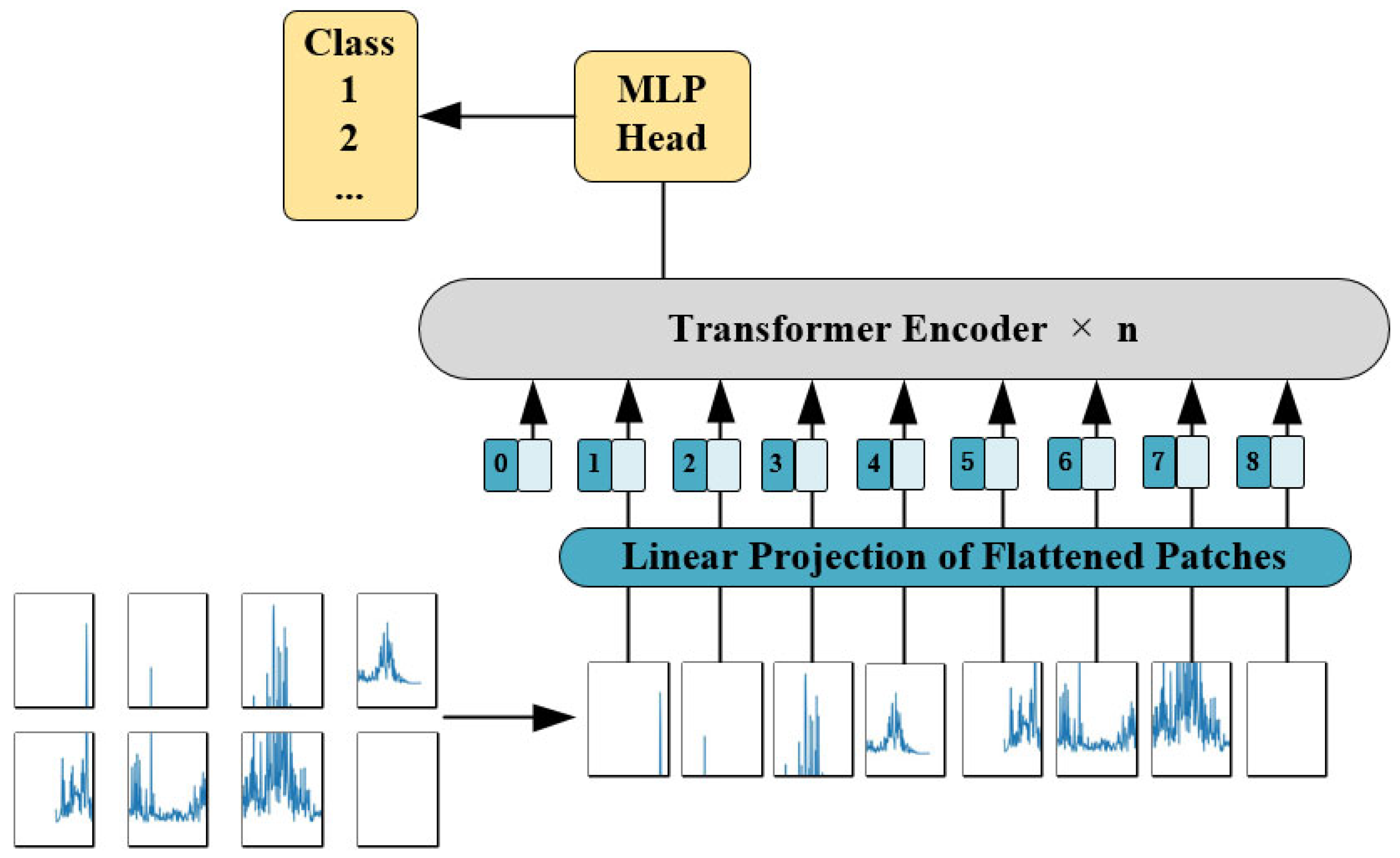
The elemental structure composition of ViT is illustrated in Figure 3. It involved five image processing steps: image pre-processing, image segmentation, encoding of positional information following segmentation, encoder encoding, and feature classification. The ViT model consisted of two main modules: the visual embedding layer and the transformer encoder layer.

(1)

Visual Embedding Layer

The visual embedding layer performed three specific tasks: image pre-processing, image segmentation, and encoding of location information after segmentation.

Task 1: Image preprocessing. The resolution of the non-uniform images was not conducive to the input of the network model. Therefore, the images required resizing to attain a resolution of 224 × 224.

Task 2: Convolution-based image segmentation. During this step, the image with a resolution of 224 × 224 was divided into equally sized blocks. Following image preprocessing, the images underwent transformation into a numerical matrix. One of the images was represented as matrix data of $A\in R^{224\times 224\times 3}$, where 224 × 224 denoted the image resolution size, and 3 referred to the number of channels. If the dimensionality of the image matrix was too large, the complexity of network model processing would be increased. To reduce the complexity of network model processing and facilitate input to the visual embedding layer, it was necessary to perform dimensionality reduction on the original image and then tile it. Because the convolution kernel had the characteristics of translation invariance and shared weights, the convolution operation was performed on the input matrix data. The process was a linear mapping process.

Table 2. Convolutional parameter settings.

Convolution Kernel Parameters	Parameter Value
Input Channel	3
Output Channel	768
Kernel Size	(16,16)
Stride	(16,16)

shows the convolution parameter settings, and Formula (5) is the convolution principle formula.

$$conv{(In,Ke)}_{x,y}={\displaystyle \sum _{i=1}^H{\displaystyle \sum _{j=1}^L{\displaystyle \sum _{k=1}^{C}K{e}_{i,j,k}I{n}_{x+i-1,y+j-1,k}(1<x,y<k}}})$$

(5)

In the formula, $H$, $L$, and $C$ indicate the height, width, and number of channels of the input image digital matrix, respectively; $k$ denotes the size of the convolution kernel; $In$ indicates the number of input channels; and $Ke$ denotes the size of the convolution kernel. The dimensionality of the matrix after convolution was calculated as follows:

$$\dim (conv(In,Ke))=\left[\frac{H+2p-k}{s}+1,\frac{W+2p-k}{s}+1\right]$$

(6)

In the formula, $p$ denotes the edge complement size, and $s$ refers to the convolution step size. Each image’s information was calculated by Formula (6) to obtain the output feature matrix $A_1\in R^{(14,14,768)}$. A piece of image information was divided into 14 × 14, for a total of 196 copies. The current 196 × 768 matrices would be spliced with a 1 × 768-dimensional classification vector to facilitate data classification. At this time, a piece of picture information would be organized into a vector of dimension 197 × 768.

Task 3: Position information encoding. Since there is a lack of practical correlation between image positions after dimension transformation, it became necessary to encode the image position information. This step helped to avoid any confusion about the output image and ensured marking of the position of every vector. A popular encoding technique is fixed position encoding using the sine–cosine function, along with relative position encoding and other forms of learning position encoding. Sine–cosine function fixed position encoding was used in the Transformer model with the following calculation:

$$P{E}_{(pos,2i)}=\sin (pos/10,{000}^{2i/d_{model}})$$

(7)

$$P{E}_{(pos,2i+1)}=\cos (pos/10,{000}^{2i/d_{model}})$$

(8)

In the formulas, $pos$ denotes the element’s position; $i$ represents the position’s encoding dimension; and $d_{model}$ is the model parameter, where the range of values is $\left[0,\dots , d_{model}/2\right)$.

(2)

Transformer Encoder Layer

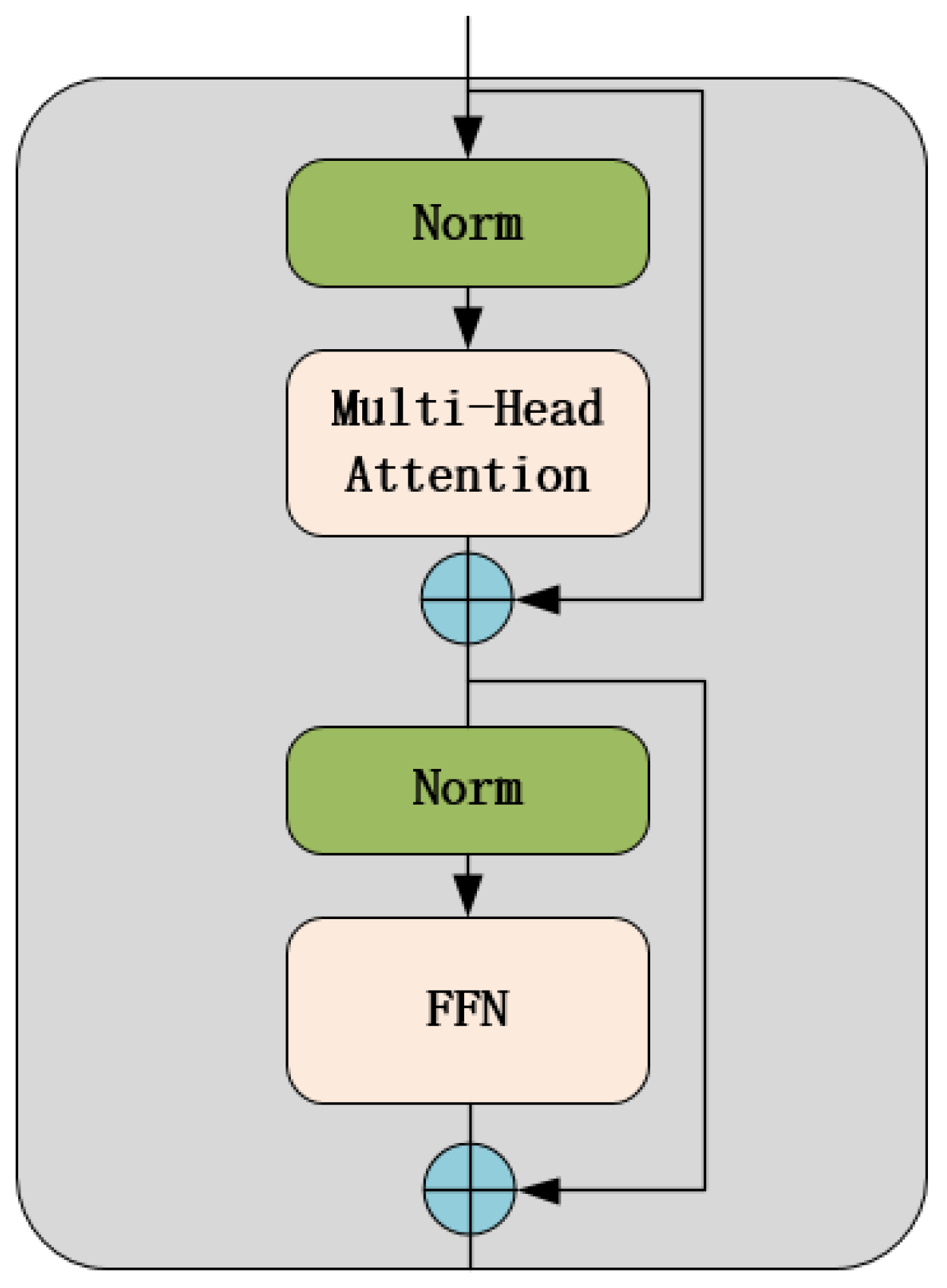
The encoding layer of ViT consisted of multiple encoders, and the encoder structure is shown in Figure 4.

The Multi-Head Attention mechanism can extract information from multiple dimensions, enrich feature diversity, and prevent overfitting, thereby improving the overall model performance. In this approach, different attention heads use various Q (query), K (key), and V (value) matrices that may be randomly initialized. The trained input vectors are projected into different subspaces, and multiple independent attention heads carry out the process in parallel. The result vectors of this process are aggregated and then mapped to the final output. The expression of the Multi-Head Attention mechanism operation is as follows:

$$Q_i=X{W}^{Q_i},K_i=Y{W}^{K_i},V_i=Y{W}^{V_i}$$

(9)

$$Z_i=Attention(Q_i,K_i,V_i),i=1\dots h$$

(10)

$$MutilHead(Q,K,V)=Concat(Z_1,Z_2,\dots ,Z_h)W^O$$

(11)

In the formulas, $i$ is the number of the attention head from 1 to $h$; $W^{Q_i}\in R^{d_{model}\times d_k}$, $W^{K_i}\in R^{d_{model}\times d_k}$, and $W^{V_i}\in R^{d_{model}\times d_v}$ denote three different linear matrices; $W^O\in R^{h{d}_v\times d_{model}}$ is the output projection matrix; and $Z_i$ refers to the output matrix of each attention head. The Multi-Head Attention mechanism separates the input into $h$ independent attention heads under the action of $d_{model}/h$ dimensional vectors and performs multi-head parallel processing of the features.

As depicted in Figure 4, the encoder comprised two residual link structures that enhanced the image information flow and contributed to improved accuracy in model training. Each residual link had a layer normalization function. The attention mechanism was applied to the first residual link, while the second residual link utilized the feedforward neural network. The Feedforward Neural Network (FFN) function is shown in Formula (12).

$$FFN(x)=\sigma (W_{1}x+b_1)W_2+b_2$$

(12)

Two linear transform layers with a nonlinear activation function formed a feedforward neural network. $W_1$ and $W_2$ in the above formula are the parameter matrices of the two linear transform layers. The activation function is usually a GELU function, denoted by $\sigma$ in the formula. $b_1$ and $b_2$ are bias parameters. The output of a single encoder can be represented by Formulas (13) and (14).

$$O_1=X+LN(MHA(X))$$

(13)

$$O_2=O_1+LN(FFN(O_1))$$

(14)

In the above two formulas, $X$ refers to the vector data entering the encoder; $LN$ refers to the layer normalization function; $MHA$ refers to the Multi-Head Attention function; $O_1$ refers to the vector data after the first residual linking process; and $O_2$ refers to the vector data after the second residual linking output, which is the data output from the encoder.

3. Fault Diagnosis Accuracy Test

To assess the effectiveness and accuracy of the proposed method, this paper examined its signal noise reduction capability and fault identification accuracy using an open-source public dataset and a rolling bearing test rig dataset.

3.1. Rolling Bearing Fault Open-Source Dataset Test

The experiment employed the rolling bearing fault open-source dataset made available by Case Western Reserve University, USA, and specifically, the SKF deep groove ball bearing model 6205-2RSJEM was selected. This bearing type is commonly used in mine hoists for high-speed and low-friction applications. The test was conducted at a load of 0 HP, a speed of 1797 r/min, with single-point failure damage diameters of 0.1778, 0.3556, and 0.5334 mm located at the inner ring, outer ring, and rolling element of the bearing. The dataset’s sampling frequency was 12 kHz, and the dataset’s sample length was 1024. Various fault datasets, including different fault types under different loads, were divided into training, validation, and testing sets using a ratio of 7:2:1.

Table 3. CWRU bearing dataset.

Fault Type	Single Point Diameter/mm	Sample Size	Category Label
normal	0	100	0
inner race	0.1778	100	1
inner race	0.3556	100	2
inner race	0.5334	100	3
outer ring	0.1778	100	4
outer ring	0.3556	100	5
outer ring	0.5334	100	6
rolling body	0.1778	100	7
rolling body	0.3556	100	8
rolling body	0.5334	100	9

provides the selection information.

Gaussian white noise was added to the original data samples to simulate data affected by noise and to test the proposed algorithm’s diagnostic performance on noisy data. The signal-to-noise ratio (SNR) was calculated as follows:

$$R_{sn}=10\lg \left(\frac{p_{signal}}{p_{noise}}\right)$$

(15)

In the formula, $R_{sn}$ indicates the SNR; $P_{signal}$ indicates the adequate power of the signal; and $P_{noise}$ indicates the effective power of the noise.

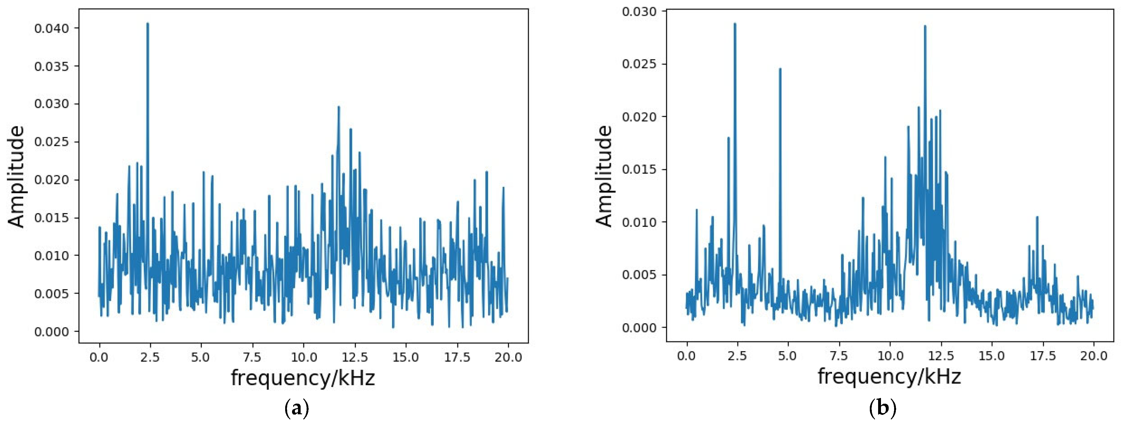
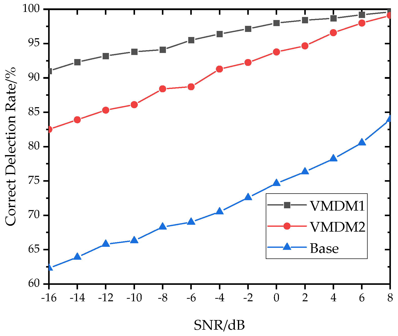
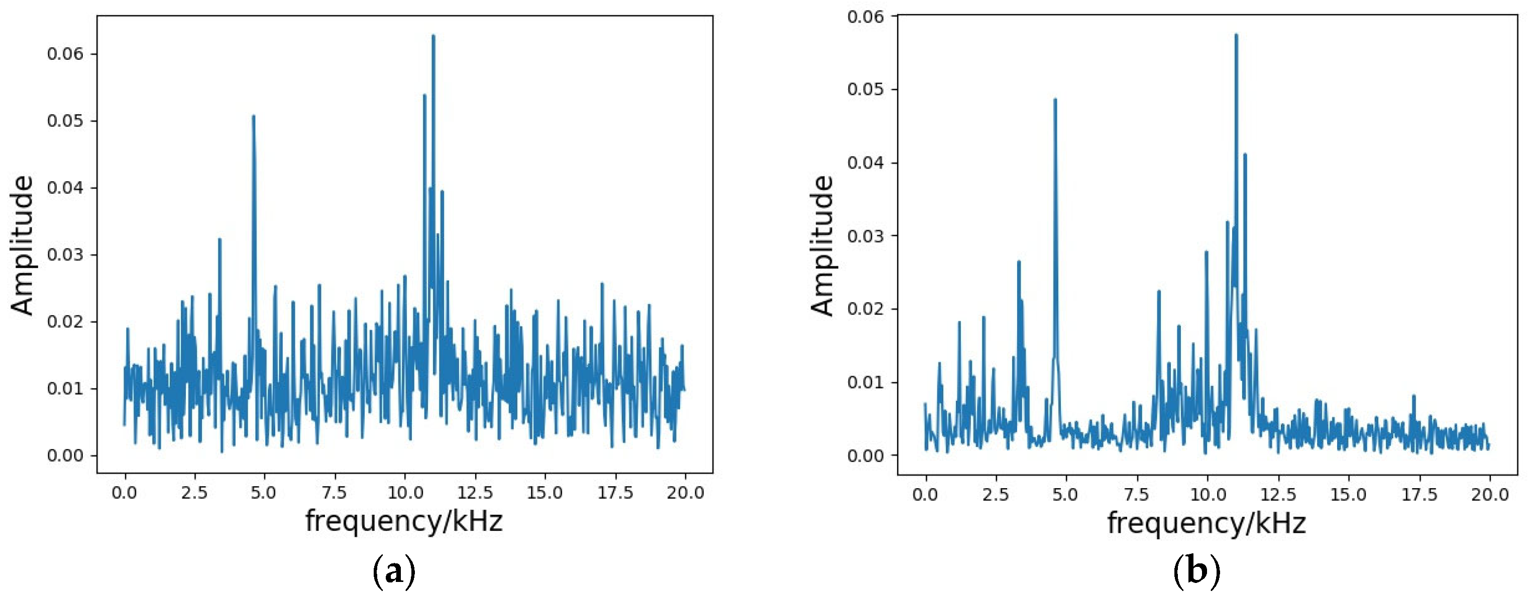
To examine the impact of the proposed improved VMD method on fault identification accuracy, the original signal with background noise (i.e., strong background noise overlaid on the original signal) and two sets of signals obtained from the improved VMD decomposition were selected and input into the ViT model for comparison. The two decomposed input signals could be categorized as follows: (i) containing only one modal component, corresponding to the maximum Pearson correlation coefficient (i.e., the maximum value), K = 1 (denoted as VMDM1); and (ii) containing two modal components, corresponding to the state component with the maximum Pearson correlation coefficient (i.e., the state component), K = 2 (denoted as VMDM2). The signal spectrum with added and reduced noise is illustrated in Figure 5. To simulate a high-intensity noise environment, the noise SNR was set to −16 to 6 dB for the original superimposed signal, and the test results are shown in Figure 6. The accuracy of the test for all types of signals decreased monotonically with increasing noise ratio. At a SNR of −2 dB, the three ViT models identified signals with 99.15%, 92.23%, and 72.65% accuracy, respectively. At a SNR of −16 dB, these accuracies dropped to 91.0%, 82.53%, and 62.3%, respectively. Among the three input signals, the fault recognition accuracy was consistently higher when a single maximum signal component was employed as compared to the other two groups. Furthermore, the model recognition accuracy was less sensitive to changes in SNR when a single maximum signal component was used, as compared to the other two groups. This suggested that during the signal decomposition process, increasing the K value, even without leading to over-decomposition, resulted in a higher number of IMFs that may have compromised the signal’s noise reduction and reconstruction quality. Consequently, under conditions where there was an increase in noise, the VMDM2 accuracy decreased more rapidly. However, decreasing noise levels led to rapid improvements in the accuracy of the VMD2 model. This phenomenon further suggested that under low noise conditions, increasing the K value could enhance model performance. However, under normal noise conditions, the improvement was limited.

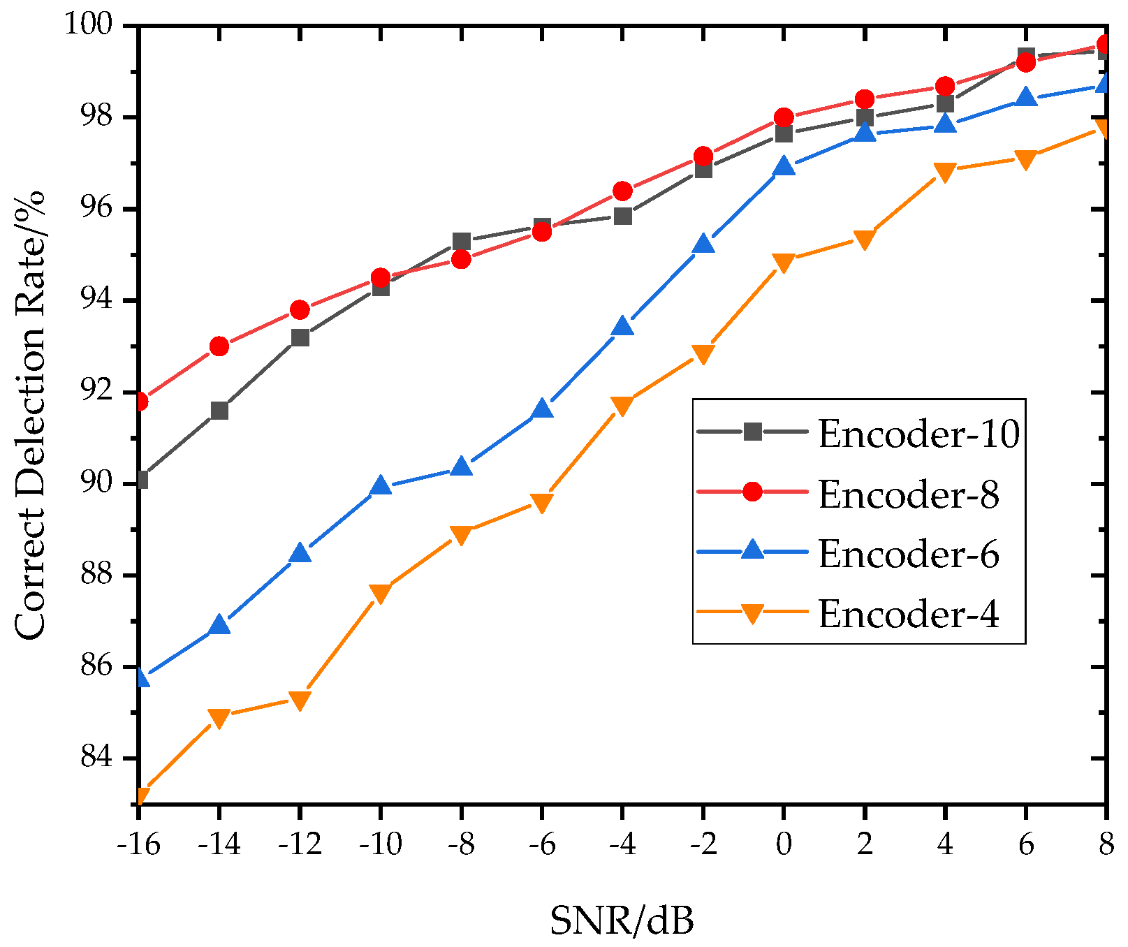
To investigate the impact of various encoding layers on fault diagnosis accuracy, the fault identification performance was evaluated using 4, 6, 8, and 10 encoders (Encoders-4/6/8/10). The sample data were tested at SNRs ranging from −16 to 8 dB. The reconstructed signal components obtained from VMDM1 decomposition were input into the ViT model for fault diagnosis analysis. The test results are shown in Figure 7. As the SNR decreased, the diagnostic accuracy for Encoder-4 experienced a more rapid decline compared to the other models. In contrast, Encoder-8 and Encoder-10 exhibited higher diagnostic accuracy, with both models having diagnostic accuracy greater than 99% at an SNR of 8 dB. However, the test accuracy of Encoder-10 was higher than that of Encoder-8 only at SNRs of −8, −6, and 8 dB. Under the remaining noise conditions, the model accuracy of Encoder-8 was higher than that of Encoder-10, and this phenomenon was more obvious in strong noise environments with SNRs of −10 to −16 dB. As depicted in the figure, model accuracy increased as the number of encoders grew from 4 to 8. However, when the number of encoders increased to 10, model performance began to decline. This was because the residual structure comprising the feedforward neural network and Multi-Head Attention mechanism in the encoder mitigated the performance degradation issue caused by encoder stacking to some extent. Appropriate encoder increases improved the model’s ability to extract features from the training data. However, crossing a certain number of encoders led to a model that was overly complex, making feature extraction in high-intensity noisy environments increasingly difficult, and replacing the training data with memory data could cause overfitting. Hence, selecting an optimal number of encoders enhanced the model’s performance and prevent overfitting.

In this paper, we employed the VMD+CNN network as a reference to evaluate the fault recognition accuracy of the proposed method under strong background noise. We compared the performance of the two methods under various SNR conditions (−16 to 8 dB) (as shown in Figure 8).

The feature recognition accuracy of VMD+CNN was 93% at −6 dB SNR, peaking at 99.40% at 8 dB SNR. The recognition accuracy of VMD+ViT could attain 95.50% at −6 dB SNR, which was comparable to that of VMD+CNN at around 5 dB SNR. However, the overall test accuracy of the VMD+ViT model was higher than that of the VMD+CNN model. Furthermore, the accuracy of the VMD+ViT model gradually increased with increasing SNR value, reaching 99.58% accuracy at 8 dB SNR. Meanwhile, Figure 8 illustrates that as the SNR decreased and the noise environment became more intense, the superiority of VMD+ViT over VMD+CNN became more apparent. When the signal-to-noise ratio dropped to −16 dB, the accuracy of the VMD+ViT model dropped to 92.7% while the accuracy of the VMD+CNN model dropped to 89.6%, thereby substantiating the dependability of using VMD+ViT for diagnosing faults in high-noise environments. Since CNN is typically insufficient for capturing long-range features of input time series and is mainly used for extracting local features from long sequences of vibration signal data, it is often necessary to incrementally perform convolutional operations layer by layer, which introduces a large number of parameters and computational effort. In contrast, ViT featured the Multi-Head Attention mechanism, which could capture global features and differentiate between the degree of contribution of individual samples to the results. The VMD+ViT method yielded excellent performance in fault diagnosis.

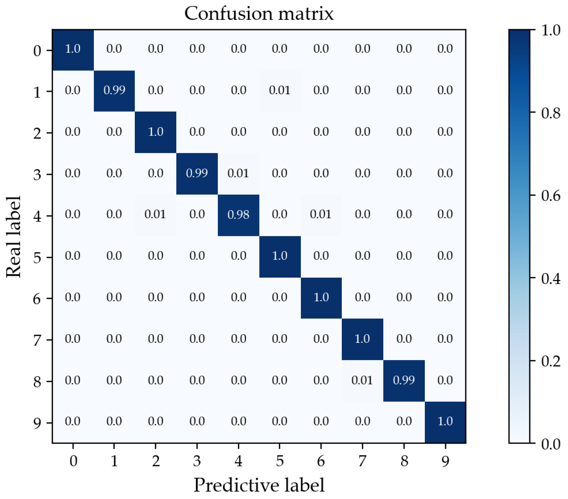
As shown in Figure 9, the confusion matrix depicts the outcome of multiple tests of the VMD+ViT model at an 8 dB signal-to-noise ratio. The horizontal coordinates of the confusion matrix indicate the predicted labels, and the vertical axes show the real labels. The figure represents ten fault categories, and only labels 1, 3, 4, and 8 achieved less than 100% recognition accuracy. Even in the datasets with the lowest recognition accuracy, these four labels still achieved above 98%. The test results indicated that the VMD+ViT rolling bearing fault diagnosis method would be highly effective in recognizing faulty deep groove ball bearings in high-speed and low-friction applications.

3.2. Fault Test Dataset Test

This section validates the feasibility of the proposed method for different types of rolling bearings of mine hoists using a fault test dataset. The test bearings employed were cylindrical roller bearings, which exhibit high load-bearing capacity and are widely used for lifting equipment in mine hoists. The tested bearing type in this study was the NU216 cylindrical roller bearing, featuring an inner ring diameter of 80 mm, an outer ring diameter of 140 mm, and a width of 26 mm. The YLP-MDF-152 three-dimensional fiber laser marking machine was utilized to create cracks and pitting defects on the inner and outer rings as well as on the rolling body of the bearing. Throughout the test, a vibration sensor gathered the fault vibration signal with a 50 kHz sampling frequency, and to simulate heavy load conditions, radial loads of 5, 7, and 9 kN were applied to the bearing at operating speeds of 800 and 2400 r/min, respectively.

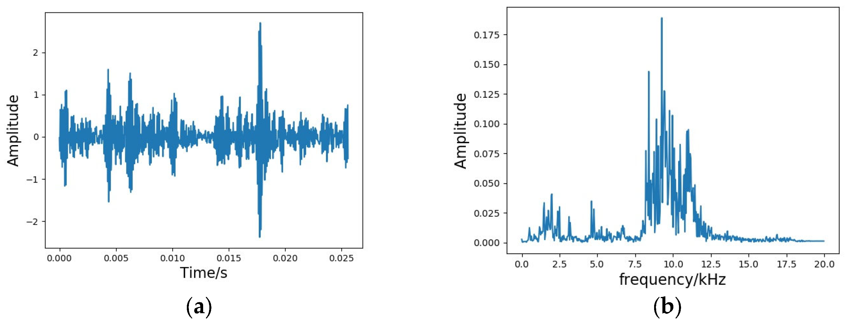
The collected vibration signal dataset contained 6 fault types, each with 100 samples and a sample size of 1024. The dataset was divided into three parts: the training, validation, and test sets in a ratio of 7:2:1. The original vibration signal was decomposed using VMD, wherein the cracked inner ring fault data at a speed of 800 r/min and load of 9 kN serves as an example. Figure 10 showcases the original and decomposed signal spectra.

The VMD-decomposed signals were fed into the ViT model to identify faults, and the diagnostic results were compared to those of alternative methods. As seen in Figure 11, the proposed method demonstrated higher diagnostic accuracy in different working conditions than the four comparison models [16,27,28].

The proposed method had the highest test accuracy in different working condition tests compared with other network models, demonstrating robustness and exceptional accuracy in addressing rolling bearing faults under noisy conditions. The CNN model was less effective at capturing long-range features in the input time series. Therefore, even though the VMD technique produced adequate de-noising results, the overall performance of the CNN model was inferior to that of ViT. The structure of LeNet-5 is relatively straightforward, which limited its ability to extract sufficient meaningful information about the bearing’s operational condition. Therefore, this technique was less effective in accurately diagnosing faults. SVM is known for its fast speed and high accuracy in classifying low-dimensional data and small samples. However, SVM’s performance is sensitive to its own parameters, and it was less effective in accurately diagnosing faults in situations involving high volumes of data or when the data contained noise. BP neural networks have a limited number of layers, which can lead to inefficient training and proneness to overfitting during training and testing, reducing their accuracy. The ViT model’s encoder structure included the residual structure of the FFN layer, which effectively resolved the issue of network degradation. Furthermore, the Multi-Head Attention mechanism enabled the model to distinguish the varying contribution levels of different samples to the results, resulting in superior diagnostic accuracy for the VMD+ViT method compared to alternative models.

The comparison of the tested accuracies of each network model in different noise environments is shown in Figure 12. The figure shows that the recognition accuracy of VMD+ViT always stayed above 90% and had the highest accuracy among all the compared models. When the SNR dropped to −12 dB, the recognition accuracy of the VMD+CNN model dropped below 90%. The recognition accuracy of LeNET-5 dropped to less than 90% when the SNR was below 0 dB. SVM and BP showed lower accuracy throughout the test. Therefore, compared with other fault diagnosis methods, the proposed method in this paper improved fault diagnosis accuracy and kept the accuracy stable under strong noise conditions.

Figure 13 depicts the confusion matrix of the proposed method’s test results, conducted under a radial load of 7 kN and operating speed of 800 r/min. The illustration highlights the VMD+ViT method’s ability to achieve high recognition accuracy for all six fault categories. Only three fault labels recorded the lowest accuracy rate of 98%, indicating exceptional performance overall. Based on the findings, the VMD+ViT method was an effective diagnostic tool for identifying cylindrical roller bearing faults in heavy load application scenarios.

4. Conclusions

To address the issue of rolling bearing fault diagnosis in mine hoists under strong noise conditions, we proposed a bearing vibration signal fault diagnosis method based on the VMD-ViT model to accurately identify fault characteristics. Below are the conclusions reached from testing the method on rolling bearing fault data using open-source and fault test datasets:

(1)

The selection of optimal parameters for VMD and ViT models must be tailored to specific application scenarios. In cases involving heavy data contamination with noise, it was found that a VMD+ViT model containing a modal component with one maximum Pearson correlation coefficient achieved higher diagnostic accuracy than a VMD+ViT model that employed an 8-Encoder structure.

(2)

The VMD+ViT model’s diagnostic method was proven to be effective in achieving fault diagnosis, even in noisy environments. In the rolling bearing open-source dataset, the diagnostic accuracy exceeded 92.70% under strong interference noise, while in bearing test datasets, the accuracy rate was over 98.62%, indicating exceptional accuracy and robustness.

(3)

When applied to rolling bearings in various working condition tests, the VMD+ViT method exhibited the highest accuracy in fault diagnosis compared to the VMD+CNN, LeNet-5, SVM, and BP methods. The proposed method can be applied to diagnosing and accurately classifying different rolling bearing fault categories in mine hoists in a strong noise environment.