Abstract
Surface topography measurements are becoming more and more popular and complement the 2D analysis of surface texture. The selection of the measurement area is not yet included in the standards, and the size of this area affects the values of the determined parameters. The article presents the results of research on determining the measurement area based on the smooth-rough crossover scale (SCR) and mean profile element spacing (Rsm) parameters. The tests focused on measuring the surface topography of random and directional types of polymer parts produced by various additive manufacturing techniques. The measurements were conducted using the focus variation method. Surface topography parameters were determined for large evaluation areas determined based on the cut-off filter length Lc and for small areas defined based on the SCR and Rsm parameters. The values of parameters determined from large areas constituted the reference values to which the values determined from small areas were compared. In the case of random-type samples, it was shown that the values of the parameters calculated from smaller areas determined based on the SCR significantly differed from the reference values. For both types of samples, determination of the evaluation area based on the Rsm yielded good results. In most cases, the greatest differences between the values of parameters calculated for small and large areas were noted for the Ssk and Smr1 parameters. Based on the test results, it could be advantageous to replace the measurement of a larger area with the measurement of several smaller areas located at different places on the sample.
1. Introduction
Additive manufacturing (AM) techniques are currently one of the fastest developing technologies used to produce even the most geometrically complex models. In additive manufacturing, before making a real object [1,2], a digital model is divided into layers. The thickness of a single layer largely depends on the implemented method of the additive manufacturing [3,4]. The model printing process consists of applying the material in layers until a complete model is obtained [5]. Depending on the manufacturing technology, the dimension of the part, and the complexity of its geometry, the complete production of a model using additive manufacturing techniques can take a few hours or even several days. Currently, there are many different methods allowing for the additive shaping of models. Taking into account the ISO/ASTM 52900 [5] and ISO/ASTM 52910 [6] standards, seven additive object manufacturing techniques can be defined: vat polymerization (VPP), powder bed fusion (PBF), material extrusion (MEX), directed energy deposition (DED), sheet lamination (SHL), material jetting (MJT), and binder jetting (BJT). The differences in how they work depend mainly on the method of solidifying successive layers as well as on the type of material used. Models produced with additive manufacturing are used in the aviation [7,8,9], automotive [10,11], medical [12,13,14], dental [15,16], architecture [17], and agriculture industries [18].
Considering the fact that fully functional models are often produced using additive technologies, conducting a thorough control of shape and dimensional accuracy [13,19,20] as well as surface roughness [21,22,23] is of great importance. Measurements are carried out using contact methods [24,25] or optical methods [26,27]. Currently, optical surface topography measurements are gaining more and more popularity [27,28,29,30]. This is the result of the developments in measuring devices, mostly optical, enabling 3D measurements of the surface texture with a very high resolution in an increasingly shorter time. However, a number of errors can often creep in when measuring surfaces using optical methods, e.g., the formation of peaks at the edges and depressions of the surface and loss of signal at the focal point of the light beam. In addition, in the case of optical methods, the measurement parameters should be adapted to the specific measured geometry [23,31,32,33]. One of the measurement parameters that affect the values of the determined parameters of the surface texture is the measurement area [23,28,31,34]. In the case of 2D profile measurements, the ISO 21920-1:2021 [35] standard contains recommendations regarding the selection of cut-off filter values and the reference and measurement length. These values refer to the Gaussian filter [36]. Although the standards of the ISO 16610 series define a number of filters that are used in 2D and 3D surface texture measurements, the most popular and widely used method currently is the aforementioned linear Gaussian filter. In the case of 3D measurements, due to the lack of formal recommendations, it is common practice to select filters and the measurement area in the same way as in the case of 2D measurements. Assuming the lengths of the sides (or only one side) of the measurement area based on the measurement length suitable for 2D measurements can lead to a relatively large area. This, in turn, may be associated with difficulties with conducting shape filtration, especially in the case of surfaces with variable curvature. Measuring a large area is also not advisable if the surface has a small radius of curvature. The measuring tip (contact or optical in the form of light) should be perpendicular to the tested surface. A large measurement area is also associated with time-consuming measurements and processing of data. The need to use a large measuring range in the vertical axis may also result in reducing the resolution of the axis. Considering the above reasons, looking for new solutions when selecting the appropriate measurement area is of great importance.
In the work [37], it was proposed that the size of the measurement area should be determined on the basis of the SCR (smooth-rough crossover scale) parameter. It is a parameter determined as a result of fractal analysis conducted using the patchwork method [38]. The application of this method to 3D surface topography measurement data consists of spreading a mesh of triangles of various sizes on them. The size of the triangles is related to the size of the scale s. Depending on the applied algorithm, the scale may express the area of a triangle or the length of one of its sides. For a mesh of triangles in a given scale, their total area is calculated. The total area of the triangles is divided by the value of the projected area. Thus, the relative area ratio AR is calculated. Then, AR values depending on the s scale are presented in a log–log chart. A linearizing straight line runs through some of the points. The value of the parameter is such a scale value, for which this line intersects the AR = 1 line. For scale values greater than the SCR, the data no longer provide new information. Information on surface irregularities is presented only for scales smaller than SCR. The size of the measurement area based on the parameter was used, e.g., in the works [21,39].
In practice, another approach is commonly used as well, involving a visual analysis of the surface. The aim is to recognize the dominant structures on the surface. The measurement area is usually chosen to contain at least five such structures. As they can be difficult to clearly identify, it is advantageous to implement this concept in order to obtain a numerical parameter. The authors concluded that the average value of the linear dimension of these dominant structures can be the Rsm (mean profile element spacing).
The article presents the results of research on the possibility of determining the size of the measurement area based on the SCR (smooth-rough crossover scale) and Rsm parameters. The values of selected 3D surface parameters of samples produced by additive methods were analysed. The test samples were made using fused deposition modelling (FDM), melted and extruded modelling (MEM), fused filament fabrication (FFF), material jetting (MJT), selective laser sintering (SLS) and multi jet fusion (MJF) methods. In the case of the SLS and MJF methods, samples after additional machining were included as well. Surface texture parameters were determined for two different sizes of the measurement area: a larger one determined based on the length of the cut-off filter, similarly as for 2D measurements, and a smaller one determined based on the SCR and Rsm parameters. The measurement of the surface texture was conducted using a focus variation microscope [40,41].
2. Materials and Methods
The research methodology from the preparation of the test samples to the measurement of the surface topography is presented in Figure 1. The measurements of the surface texture were carried out on the samples that can be classified as random/isotropic (A samples) and directional (B samples). A samples were manufactured by MJF and SLS methods. In the case of the SLS method, the EOS P 396 3D printer was used, and in the case of the MJF method, the HP MJF 5200 3D printer was used. For both 3D printers, standard manufacturing parameters were selected for the PA12 material (Table 1). The obtained samples were rectangular with dimensions of 40 mm × 40 mm × 4 mm. The 40 mm × 40 mm surfaces were parallel to the XY planes of the printers. With these samples, measurements of the surface texture were conducted on the upper surface of 40 mm × 40 mm.
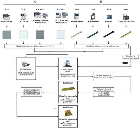
Figure 1.
Scheme of research.

Table 1.
Parameters of manufacturing test samples.
Then, the produced test samples were subjected to mechanical smoothing as well. For this purpose, the DyeMansion Powershot C was used (samples MJF+PC and SLS+PC in Figure 1). DyeMansion Powershot C is equipped with a rotating basket and is manufactured from stainless steel. Two simultaneously working blasting nozzles positioned perpendicularly to the rotating basket and the contained parts efficiently remove the powder. A fixed distance between the elements and the blasting nozzles ensures reproducible results with no risk of damaging the components during the process [42]. Glass beads (200–300 m) were used in the process. The mechanical processing time was 5 min at 3 bar pressure.
Type-B samples were cylinders with a diameter of 8 mm and spheres with a diameter of 12 mm. They were produced with MEM, FFF, FDM, and MJT methods. The parameters of the printed samples are presented in Table 2. The samples during printing were oriented in the same way—the axis of the cylinder was aligned with the vertical axis of the given 3D printer. Due to the optical properties of the samples produced with FDM, FFF, MEM, and MJT methods, replicas of their surfaces made of RepliSet-F5 silicone mass were used for optical surface roughness measurements.
Table 2.
Measurement parameters of the surface topography using focus variation microscope.
For each type of test sample, attempts were made to determine the parameters of the surface topography from areas of various sizes. The surface topography was measured with the Alicona InfiniteFocus G4 focus-variation microscope. However, before the measurements with the microscope, the test samples were measured three times with the 2D MarSurf M300 profilometer in order to initially determine the measurement length and to estimate the Ra, Rq, Rz, and Rsm parameters, which were used to select the appropriate objective and measurement parameters for the Alicona microscope. At this stage of the measurements, the measurement length was selected automatically by the profilometer software. Due to the excessively large curvature of the surface, measuring the 12 spherical samples proved to be impossible. The length of the measurement for these surfaces was assumed to be the same as for the surfaces of the cylindrical samples made by the same method. As a result, for all surfaces, the measurement length determined in the presented way was equal to 4 mm.
A fragment of the sample surface was measured with the InfiniteFocus G4 focus-variation microscope in such a way that in the X direction the measurement area was at least 4 mm long. The size of the measurement area in the Y direction resulted from the adopted objective; for A samples, it was equal to 0.5 mm, and for B samples, it was equal to 1 mm. The surface topography measurement parameters are presented in Table 2.
Subsequently, the measurement data were processed with the SPIP 6.4.2. software. In the case of flat samples, the data were levelled to the surface (global levelling), and in the case of spherical and cylindrical samples, the shape was filtered (form was removed) using a second-degree polynomial function. Then, based on a visual assessment, the length of the cut-off filter Lc was selected to separate the waviness components. At this stage, selected lengths specified in the ISO 21920 standard were tested, i.e., 0.25 mm, 0.8 mm, and 2.5 mm. For all tested samples, 0.8 mm proved to be the most suitable filter length. Finally, a larger measurement area assumed an area with 4 mm of length in the X direction (0.8 mm × 5). For each test sample, two such areas were measured. For each area, the parameter and the average Rsm value calculated based on 10 profiles were determined. The average values of these parameters are presented in Table 3. In order to determine the length of the measurement area in the X axis based on the SCR and Rsm, the values of these parameters were multiplied by 5 and rounded up to the nearest decimal value. In the case of B samples, the lengths of 5 × SCR were typically only 0.1 mm shorter than 5 × Rsm. On the other hand, for A samples, the differences between SCR and Rsm were much greater. The calculated values of 5 × Rsm were 1.8 to 4.5 times greater than 5 × SCR.
Table 3.
Values of SCR and Rsm parameters determined from large measurement areas and dimensions of small measurement areas.
The measured large fragments of the topography (without filtration) were then divided into smaller parts of the size corresponding to the small area determined based on Rsm or SCR. For example, in the case of a cylindrical FFF sample, the small area determined from Rsm was 0.9 mm × 1 mm. From one large measured area of 4 mm × 1 mm, 4 small fragments were isolated. Each large and small fragment was subjected to shape and waviness filtration (Lc mm). For both large and small fragments after filtration, surface topography parameters were determined. In the study, the most commonly used parameters in industrial practice were analysed [43]: Sa, Sz, Sq, Sp, Sv, Sku, Ssk, Spk, Sk, Svk, Smr1, Smr2, Sdq, Sdr, Sds, Sal, and Str [44]. For each type of test sample and each analysed parameter, the following values were determined:
- —the relative difference between the results obtained for two 4 mm × 1 mm surfaces, e.g., for the Sa parameter:where and are the values of Sa for largest and second-largest areas, respectively.
- —the relative difference between the results obtained for a large area and a small area isolated from it:where is the i-th large area, and is the j-th area isolated from the i-th large area.
- —the average of the relative differences :
- a difference equals:
A positive d value for a given parameter can be interpreted as an indication that the values of this parameter for two large areas measured on the same test sample differ more than the values of the parameter calculated for small areas compared to the value determined for the large area. In other words, the difference in the parameter value resulting from the measurement of the smaller area is greater than the difference resulting from measuring the topography at different places on the test sample. In order to test if the measurement of a smaller measurement area does not negatively affect the determined topography parameters, the values of d should not be too large. In the tests, it was assumed that the value of % indicates that the decrease in the measurement area does not significantly affect the value of a given parameter. However, in the case of %, the influence of the size of the area was considered to be too great. The 5% and 10% values refer to levels of statistical significance commonly used in scientific research. More strict values apply to research whose results may have a direct impact on human health and safety.
The research methodology described above was adopted so that the differences , i.e., the values obtained from a small area compared to a large one, consider the fact that the effects of shape filtration and Lc filtration on large and small areas will be different. However, the research was supplemented by examining the differences in filtration results depending on the size of the measurement area. The tests were conducted with SLS+PC samples (type-A samples) and spherical MJ (type-B samples). For these samples, taking into consideration their type, the smallest evaluation areas were defined (small area (SCR) in Table 3). Three areas of 1.4 mm × 1 mm were measured on the SLS+PC sample. On the MJ spherical sample, five areas of 1.4 mm × 1 mm were measured. Then, the measurement data were processed in two ways:
- Shape filtered (from removed), Lc filter used, small area based on selected SCR, topography parameters determined for small areas;
- small area based on SCR selected, shape filtered (from removed), Lc filter used, topography parameters determined for small areas.
For each type of the sample, 10 small fragments of surface topography were analysed. Each such fragment was analysed in the two ways described above, i.e., using Lc for a large area (before a small area was defined) and using Lc for a small area.
3. Results and Discussion
In the case of the SLS+PC sample, the statistical analysis (the paired t-test with the level of significance ) did not indicate statistically significant differences between the analysed topography parameters depending on the use of filters in the area of 0.4 mm × 0.5 mm or 1.4 mm × 1 mm. However, statistically significant differences were obtained in the case of the MJ sphere in regard to Sa, Sq and Sv parameters. After applying filtration for large areas, the values of the Sa and Sq parameters were on average 1.2% higher, and the Sv parameter was 2.7% higher than the values obtained after filtration conducted for small areas. Figure 2 presents valuses of Sa depending on the use of filters in lagre or small area.
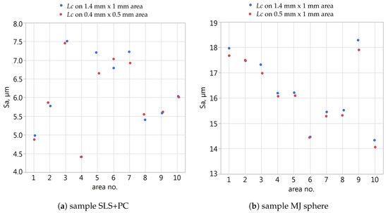
Figure 2.
Values of the Sa parameter depending on the application of the Lc filter for the 1.4 mm × 1 mm area or for the small area based on SCR.
Figure 3 and Figure 4 present views of the measured large areas of the samples, the dimension of which in the X direction equals 4 mm and small areas based on Rsm parameter. Surfaces manufactured by SLS and MJF methods (without and after mechanical smoothing, Figure 3) are random, isotropic. The maps of surfaces without mechanical smoothing show grains of bounded powder. The linear dimensions of these grains are approx. 40–80 m. There are no distinct differences between the topography of the SLS and MJF samples.
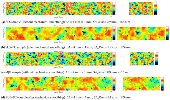
Figure 3.
Maps of the large measured areas (LA) and small measured areas based on Rsm (SA_Rsm) of samples A (after form removal and filtering using Lc mm).
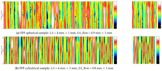
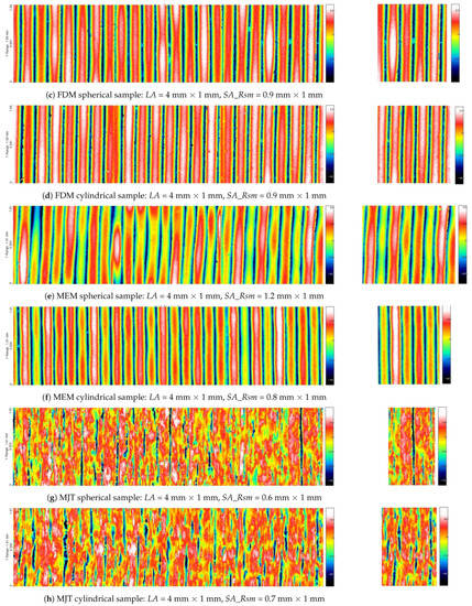
Figure 4.
Maps of the large measured areas (LA) and small measured areas based on Rsm (SA_Rsm) of samples B (after form removal and filtering using Lc mm).
The elevations visible in the topography maps of SLS and MJF samples after mechanical smoothing have much larger dimensions than single grains. After mechanical smoothing, there are also no distinct differences between the topography of the SLS and MJF samples. The views of the surfaces of B samples (Figure 4) confirm their directional properties. On the surfaces of the MEM, FDM, and FFF samples, individual layers are clearly visible. There are no distinct differences between the topography of spherical and cylindrical samples made using a given additive method.
Because the sizes of the areas determined based on SCR and Rsm for B samples were in most cases very similar, analyses were performed for surface A only. The values of are presented in Figure 5. In the case of analyses performed taking into account the parameters, the values of % and % were exceeded in over 27% and as much as 55% of cases, respectively. Basing the selection of the measurement area on the Rsm value, it was approx. 6% and 17%. It was therefore concluded that the decrease in the size of the analysed areas based on the SCR had a significant impact on the values of the determined parameters. More detailed analyses, including the B-type samples with a directional texture, were conducted only for areas determined based on the Rsm parameter.
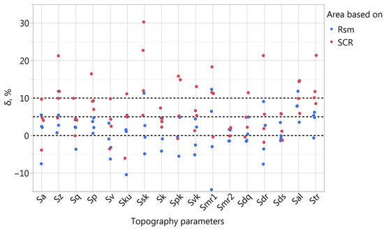
Figure 5.
Parameter values in case of A sample analysis and areas determined based on SCR and Rsm parameters.
The values of for the areas determined based on the Rsm parameter for samples A and B are presented in Figure 6 and Figure 7. In order to better visualize positive values for B samples, a logarithmic scale was used.
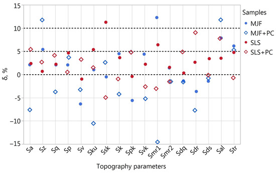
Figure 6.
Parameter values in the case of analysis of A samples area determined based on the Rsm parameter.
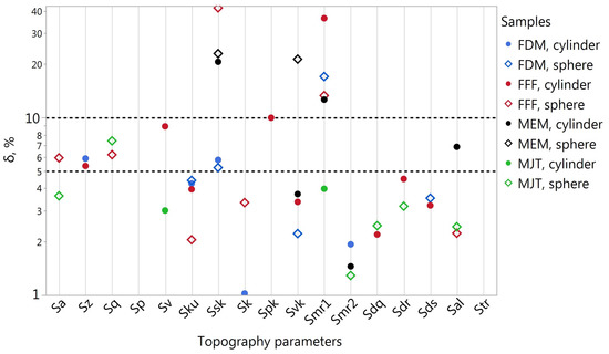
Figure 7.
Values of the parameter % in the case of analysis of B samples determined based on the Rsm parameter.
For A and B samples exceeding the limit of % occurred in 6.25% of the cases (12 times in total). Most often, it concerned the Smr1 (five times) and Ssk (three times) parameters. The values of less than 5% were observed in almost 83% of the cases for the A samples and 86% for the B samples.
Figure 8 and Figure 9 present the differences and for selected topography parameters of samples with an isotropic and directional texture. Descriptive statistics for these values for A and B samples are presented in Table 4. In the case of isotropic samples, value was greater than for all the parameters. All quantiles and the mean value presented in Table 4 for A samples are about twice as large for the parameter. In the case of samples with a clearly directional texture, the tendency was the opposite; for all the parameters except Smr1, the difference was greater than .
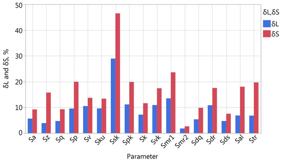
Figure 8.
Values of and in the case of analysis of A samples ( determined based on the Rsm parameter).
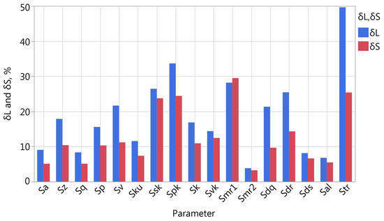
Figure 9.
Values of and in the case of analysis of B samples ( determined based on the Rsm parameter).
Table 4.
Basic descriptive statistics of and parameters determined for samples A and B.
Comparing the values for A and B samples, it can be seen that for samples with a directional texture, the values are higher. This proves that the measured fragments of the surface of isotropic samples were characterized by greater homogeneity within a given sample. The topography of samples with a directional texture was more varied depending on the location of the measurement area. Therefore, in general for samples type A and B, the above analyses show that for A samples, a greater change in the parameter values was observed by reducing the analysed area than by conducting the measurements in different locations on the sample. In the case of samples with a directional texture, in terms of representativeness of measurements, a more important aspect would be to conduct measurements in various locations than to reduce the size of the measurement area from the size based on Lc to one based on Rsm.
4. Conclusions
Surface texture is one of the crucial factors influencing the functional properties of machine parts. It applies to all types of surfaces, including those of parts produced by additive manufacturing. Although surface topography measurement methods are becoming more and more popular, the selection of the measurement area still proves to be an issue. The size of the measurement area impacts the determined values of the parameters of the surface texture.
It can be considered that measuring the topography of a larger surface area is more reliable: more data are obtained from a large area than from a small one. However, measuring a large surface area to evaluate the surface microgeometry is time-consuming and therefore costly. In addition, problems with shape filtering are more common with large measurement areas than with small ones. On the other hand, measuring too small of an area may result in problems with filtering the waviness components. When measuring too small of an area, not enough information about the surface is obtained and, for example, the values of the amplitude parameters Sp or Sz may be underestimated.
In the presented paper, the authors determined the parameters of the surface texture of the samples for measurement areas of various sizes: a larger area determined based on the length of the cut-off filter Lc (similarly as for 2D parameters) and a smaller area determined based on the SCR and Rsm parameters. Large evaluation areas (determined based on Lc) were assumed as more representative, and the parameter values determined from them served as a reference for the values determined from small evaluation areas. In the case of samples with a directional texture (B samples), the sizes of small areas determined based on the SCR and Rsm parameters were in most cases very similar. In the case of samples with random texture (A samples), significant differences were observed; the areas determined based on Rsm were 1.8–4.5 times larger than the areas determined based on the SCR.
Based on the analyses conducted for A samples, it was proven that the parameter values calculated from the evaluation area determined based on the SCR parameter significantly differ from the values determined from a large area. Assuming that the parameter values determined from a large area are more reliable, it can be concluded that the evaluation areas determined based on the SCR parameter in the case of A samples were too small. The obtained results indicate that determining the size of the evaluation area based on the Rsm parameter rather than on the SCR was preferable.
Taking into account the results obtained for all samples, it can be concluded that the values of topography parameters determined for the measurement area selected based on Lc are usually not significantly different from the values determined for smaller areas determined based on the Rsm parameter. It should be noted that the analysed delta parameter considered the average of differences determined based on measurements of several smaller areas. Therefore, the obtained results should not be interpreted in such a way that the measurement of a larger area can be successfully replaced with the measurement of only one smaller area. However, replacing the measurement of a larger area with the measurement of several smaller areas located in different places on the sample should be considered. It can provide additional information on the variability of parameters within the sample. In many cases, conducting measurements of several smaller areas proves to be easier and quicker than that of a larger area. For the samples analysed, greater variability of topography parameters within a single sample was observed on samples with a directional texture; the average value for type-B samples was more than twice as high as for type A samples. Thus, for B samples, reducing the measurement area in favour of a larger number of measurement locations could increase the representativeness of the measurements.
The conducted research does not exhaust the subject concerning the appropriate selection of the measurement area of the surface topography. Future research should focus on determining the usefulness of the Rsm parameter for this purpose, as well as trying to find alternative solutions to the discussed problem.
Author Contributions
Conceptualization, A.B., P.T. and P.S.; methodology, A.B., P.T. and P.S.; investigation, A.B., P.T. and P.S.; resources, Ł.P. and A.Z.; writing—original draft preparation, A.B., P.T. and P.S.; writing—review and editing, A.B., P.T. and P.S. All authors have read and agreed to the published version of the manuscript.
Funding
This research received no external funding.
Data Availability Statement
Data can be made available on request.
Conflicts of Interest
The authors declare no conflict of interest.
References
- Ngo, T.D.; Kashani, A.; Imbalzano, G.; Nguyen, K.T.; Hui, D. Additive manufacturing (3D printing): A review of materials, methods, applications and challenges. Compos. Part B Eng. 2018, 143, 172–196. [Google Scholar] [CrossRef]
- Gardan, J. Additive manufacturing technologies. In Additive Manufacturing Handbook; CRC Press: Boca Raton, FL, USA, 2017; pp. 149–168. [Google Scholar] [CrossRef]
- Thompson, M.K.; Moroni, G.; Vaneker, T.; Fadel, G.; Campbell, R.I.; Gibson, I.; Bernard, A.; Schulz, J.; Graf, P.; Ahuja, B.; et al. Design for Additive Manufacturing: Trends, opportunities, considerations, and constraints. CIRP Ann. 2016, 65, 737–760. [Google Scholar] [CrossRef]
- Gibson, I.; Rosen, D.W.; Stucker, B. Additive Manufacturing Technologies; Springer: New York, NY, USA, 2010. [Google Scholar] [CrossRef]
- ISO/ASTM 52900:2021; Additive Manufacturing—General Principles—Fundamentals and Vocabulary. ISO: Geneva, Switzerland, 2021.
- ISO/ASTM 52910:2018; Additive Manufacturing—Design—Requirements, Guidelines and Recommendations. ISO: Geneva, Switzerland, 2018.
- Chu, M.Q.; Wang, L.; Ding, H.Y.; Sun, Z.G. Additive Manufacturing for Aerospace Application. Appl. Mech. Mater. 2015, 798, 457–461. [Google Scholar] [CrossRef]
- Rokicki, P.; Budzik, G.; Kubiak, K.; Dziubek, T.; Zaborniak, M.; Kozik, B.; Bernaczek, J.; Przeszlowski, L.; Nowotnik, A. The assessment of geometric accuracy of aircraft engine blades with the use of an optical coordinate scanner. Aircr. Eng. Aerosp. Technol. 2016, 88, 374–381. [Google Scholar] [CrossRef]
- Gisario, A.; Kazarian, M.; Martina, F.; Mehrpouya, M. Metal additive manufacturing in the commercial aviation industry: A review. J. Manuf. Syst. 2019, 53, 124–149. [Google Scholar] [CrossRef]
- Leal, R.; Barreiros, F.M.; Alves, L.; Romeiro, F.; Vasco, J.C.; Santos, M.; Marto, C. Additive manufacturing tooling for the automotive industry. Int. J. Adv. Manuf. Technol. 2017, 92, 1671–1676. [Google Scholar] [CrossRef]
- Negrea, A.P.; Cojanu, V. Innovation as Entrepreneurial Drives in the Romanian Automotive Industry. J. Econ. Bus. Manag. 2016, 4, 58–64. [Google Scholar] [CrossRef]
- Salmi, M. Additive Manufacturing Processes in Medical Applications. Materials 2021, 14, 191. [Google Scholar] [CrossRef]
- Turek, P.; Budzik, G. Estimating the Accuracy of Mandible Anatomical Models Manufactured Using Material Extrusion Methods. Polymers 2021, 13, 2271. [Google Scholar] [CrossRef]
- Turek, P.; Budzik, G. Development of a procedure for increasing the accuracy of the reconstruction and triangulation process of the cranial vault geometry for additive manufacturing. In Facta Universitatis, Series: Mechanical Engineering; University of Nis: Nis, Serbia, 2022. [Google Scholar]
- Kwon, S.Y.; Kim, Y.; Ahn, H.W.; Kim, K.B.; Chung, K.R.; Kim, S.H. Computer-Aided Designing and Manufacturing of Lingual Fixed Orthodontic Appliance Using 2D/3D Registration Software and Rapid Prototyping. Int. J. Dent. 2014, 2014, 164164. [Google Scholar] [CrossRef]
- Martorelli, M.; Gerbino, S.; Giudice, M.; Ausiello, P. A comparison between customized clear and removable orthodontic appliances manufactured using RP and CNC techniques. Dent. Mater. 2013, 29, e1–e10. [Google Scholar] [CrossRef]
- Acher, M.; Cleve, A.; Collet, P.; Merle, P.; Duchien, L.; Lahire, P. Reverse Engineering Architectural Feature Models. In Software Architecture; Springer: Berlin/Heidelberg, Germany, 2011; pp. 220–235. [Google Scholar] [CrossRef]
- Javaid, M.; Haleem, A. Using additive manufacturing applications for design and development of food and agricultural equipments. Int. J. Mater. Prod. Technol. 2019, 58, 225. [Google Scholar] [CrossRef]
- Budzik, G.; Woźniak, J.; Paszkiewicz, A.; Przeszłowski, Ł.; Dziubek, T.; Dębski, M. Methodology for the Quality Control Process of Additive Manufacturing Products Made of Polymer Materials. Materials 2021, 14, 2202. [Google Scholar] [CrossRef] [PubMed]
- Bazan, A.; Turek, P.; Przeszłowski, Ł. Assessment of InfiniteFocus system measurement errors in testing the accuracy of crown and tooth body model. J. Mech. Sci. Technol. 2021, 35, 1167–1176. [Google Scholar] [CrossRef]
- Bazan, A.; Turek, P.; Przeszłowski, Ł. Comparison of the contact and focus variation measurement methods in the process of surface topography evaluation of additively manufactured models with different geometry complexity. Surf. Topogr. Metrol. Prop. 2022, 10, 035021. [Google Scholar] [CrossRef]
- Kozior, T.; Adamczak, S. Amplitude Surface Texture Parameters of Models Manufactured by FDM Technology. In Proceedings of the International Symposium for Production Research 2018; Springer International Publishing: Cham, Switzerland, 2018; pp. 208–217. [Google Scholar] [CrossRef]
- Leach, R.; Bourell, D.; Carmignato, S.; Donmez, A.; Senin, N.; Dewulf, W. Geometrical metrology for metal additive manufacturing. CIRP Ann. 2019, 68, 677–700. [Google Scholar] [CrossRef]
- Józwik, J. Analysis of the Effect of Trochoidal Milling on the Surface Roughness of Aluminium Alloys after Milling. Manuf. Technol. 2019, 19, 772–779. [Google Scholar] [CrossRef]
- Magdziak, M. Determining the strategy of contact measurements based on results of non-contact coordinate measurements. Procedia Manuf. 2020, 51, 337–344. [Google Scholar] [CrossRef]
- Dziubek, T.; Oleksy, M. Application of ATOS II optical system in the techniques of rapid prototyping of epoxy resin-based gear models. Polimery 2017, 62, 44–52. [Google Scholar] [CrossRef]
- Leach, R. Advances in Optical Surface Texture Metrology; IOP Publishing Ltd.: Bristol, UK, 2020. [Google Scholar] [CrossRef]
- Leach, R. (Ed.) Optical Measurement of Surface Topography; Springer: Berlin/Heidelberg, Germany, 2011. [Google Scholar] [CrossRef]
- Bazan, A.; Kawalec, A.; Rydzak, T.; Kubik, P.; Olko, A. Determination of Selected Texture Features on a Single-Layer Grinding Wheel Active Surface for Tracking Their Changes as a Result of Wear. Materials 2020, 14, 6. [Google Scholar] [CrossRef]
- Launhardt, M.; Wörz, A.; Loderer, A.; Laumer, T.; Drummer, D.; Hausotte, T.; Schmidt, M. Detecting surface roughness on SLS parts with various measuring techniques. Polym. Test. 2016, 53, 217–226. [Google Scholar] [CrossRef]
- Pawlus, P.; Reizer, R.; Wieczorowski, M.; Krolczyk, G. Study of surface texture measurement errors. Measurement 2023, 210, 112568. [Google Scholar] [CrossRef]
- Zheng, Y.; Zhang, X.; Wang, S.; Li, Q.; Qin, H.; Li, B. Similarity evaluation of topography measurement results by different optical metrology technologies for additive manufactured parts. Opt. Lasers Eng. 2020, 126, 105920. [Google Scholar] [CrossRef]
- Leksycki, K.; Królczyk, J.B. Comparative assessment of the surface topography for different optical profilometry techniques after dry turning of Ti6Al4V titanium alloy. Measurement 2021, 169, 108378. [Google Scholar] [CrossRef]
- Molnár, V. Minimization Method for 3D Surface Roughness Evaluation Area. Machines 2021, 9, 192. [Google Scholar] [CrossRef]
- ISO 21920-1:2021; Geometrical Product Specifications (GPS)—Surface Texture: Profile—Part 1: Indication of Surface Texture. ISO: Geneva, Switzerland, 2021.
- ISO 16610-21:2011; Geometrical Product Specifications (GPS)—Filtration—Part 21: Linear Profile Filters: Gaussian Filters. ISO: Geneva, Switzerland, 2011.
- Brown, C.A. Areal Fractal Methods. In Characterisation of Areal Surface Texture; Springer: Berlin/Heidelberg, Germany, 2013; pp. 129–153. [Google Scholar] [CrossRef]
- Brown, C.; Charles, P.; Johnsen, W.; Chesters, S. Fractal analysis of topographic data by the patchwork method. Wear 1993, 161, 61–67. [Google Scholar] [CrossRef]
- Triantaphyllou, A.; Giusca, C.L.; Macaulay, G.D.; Roerig, F.; Hoebel, M.; Leach, R.K.; Tomita, B.; Milne, K.A. Surface texture measurement for additive manufacturing. Surf. Topogr. Metrol. Prop. 2015, 3, 024002. [Google Scholar] [CrossRef]
- Newton, L.; Senin, N.; Gomez, C.; Danzl, R.; Helmli, F.; Blunt, L.; Leach, R. Areal topography measurement of metal additive surfaces using focus variation microscopy. Addit. Manuf. 2019, 25, 365–389. [Google Scholar] [CrossRef]
- Danzl, R.; Helmli, F.; Scherer, S. Focus Variation—A Robust Technology for High Resolution Optical 3D Surface Metrology. Stroj. Vestn. J. Mech. Eng. 2011, 2011, 245–256. [Google Scholar] [CrossRef]
- Available online: https://plmgroup.eu/wp-content/uploads/Dymansion-Powershot-C.pdf (accessed on 26 April 2023).
- Todhunter, L.; Leach, R.; Lawes, S.; Blateyron, F. Industrial survey of ISO surface texture parameters. CIRP J. Manuf. Sci. Technol. 2017, 19, 84–92. [Google Scholar] [CrossRef]
- ISO 25178-2:2012; Geometrical Product Specifications (GPS). Surface Texture. Areal. Terms, Definitions and Surface Texture Parameters. ISO: Geneva, Switzerland, 2012. [CrossRef]
Disclaimer/Publisher’s Note: The statements, opinions and data contained in all publications are solely those of the individual author(s) and contributor(s) and not of MDPI and/or the editor(s). MDPI and/or the editor(s) disclaim responsibility for any injury to people or property resulting from any ideas, methods, instructions or products referred to in the content. |
© 2023 by the authors. Licensee MDPI, Basel, Switzerland. This article is an open access article distributed under the terms and conditions of the Creative Commons Attribution (CC BY) license (https://creativecommons.org/licenses/by/4.0/).