Advancing Simultaneous Localization and Mapping with Multi-Sensor Fusion and Point Cloud De-Distortion

Abstract

This study addresses the challenges associated with incomplete or missing information in obstacle detection methods that employ a single sensor. Additionally, it tackles the issue of motion distortion in LiDAR point cloud data during synchronization and mapping in complex environments. The research introduces two significant contributions. Firstly, a novel obstacle detection method, named the point-map fusion (PMF) algorithm, was proposed. This method integrates point cloud data from the LiDAR, camera, and odometer, along with local grid maps. The PMF algorithm consists of two components: the point-fusion (PF) algorithm, which combines LiDAR point cloud data and camera laser-like point cloud data through a point cloud library (PCL) format conversion and concatenation, and selects the most proximate point cloud to the quadruped robot dog as the valid data; and the map-fusion (MF) algorithm, which incorporates local grid maps acquired using the Gmapping and OctoMap algorithms, leveraging Bayesian estimation theory. The local grid maps obtained by the Gmapping and OctoMap algorithms are denoted as map A and map B, respectively. This sophisticated methodology enables seamless map fusion, which significantly enhances the precision and reliability of the approach. Secondly, a motion distortion removal (MDR) method for LiDAR point cloud data based on odometer readings was proposed. The MDR method utilizes legged odometer data for linear data interpolation of the original distorted LiDAR point cloud data, facilitating the determination of the corresponding pose of the quadruped robot dog. Subsequently, the LiDAR point cloud data are then transformed to the quadruped robot dog coordinate system, efficiently mitigating motion distortion. Experimental results demonstrated that the proposed PMF algorithm achieved a 50% improvement in success rate compared to using only LiDAR or the PF algorithm in isolation, while the MDR algorithm enhanced mapping accuracy by 45.9% when motion distortion was taken into account. The effectiveness of the proposed methods was confirmed through rigorous experimentation.

1. Introduction

The advancement of obstacle detection through the fusion of LiDAR and camera data represents a vital area of research aimed at improving the precision of simultaneous localization and mapping (SLAM), as well as for navigation obstacle avoidance. However, the integration of 2D LiDAR and depth cameras for obstacle detection presents significant challenges, including the accurate construction of obstacle contour information within the map, and the mitigation of LiDAR point cloud distortion triggered by movement and vibrations on unstable platforms. Those issues, coupled with the resultant SLAM map drift and scale distortion emanating from point cloud distortion, necessitate further research and investigation.

Jiang [1] proposed a 2.5D map construction method that utilizes visual features for loop closure detection. López E [2], on the other hand, implemented an EKF filter that fuses LiDAR, monocular camera, and IMU data to generate a local 2.5D map. Unlike conventional 2D maps, 2.5D maps can provide height information of obstacles, while also allowing for the construction of their outlines. However, in scenarios with complex environments or expansive spaces, 2.5D maps with rich point cloud or elevation information can occupy significant memory space and incur high computational costs, resulting in decreased map accuracy and update frequencies. Consequently, this method is best suited for the construction of local maps for navigation, obstacle avoidance, or quadruped gait adaptation planning, such as Spot [3] and ANY mal [4] quadruped robots that perceive terrain and construct local elevation maps centered on the robot for adaptive gait planning and local navigation using a combination of depth cameras and LiDAR fusion. Spot Mini [5] and Mini Cheetah [6,7] quadruped robots, on the other hand, use multiple sets of cameras to sense terrain and construct similar local elevation maps.

Barbosa [8] fused 2D LiDAR and camera data using a convolutional neural network for segmentation tasks, and improved the obstacle detection accuracy for driving vehicles under adverse weather and strong lighting conditions. Wang [9] proposed an obstacle detection method based on machine learning and improved VIDAR. Specific types of obstacles were detected using machine learning algorithms, and the improved VIDAR removed unknown obstacles from the image to increase detection speed (average detection time of 0.316 s) and performance (accuracy of 92.7%). Alfred [10] proposed a pedestrian detection algorithm based on fully convolutional neural networks, which accurately locates pedestrians within a 10–30 m range using fused data from LiDAR and cameras. The fusion method based on deep learning detects and identifies specific types of obstacles through model training. The detection efficiency and accuracy are high, but it is difficult to construct an environmental map. Point cloud fusion and local grid map fusion are still the mainstream fusion methods. Xiao [11] lowered the cost of 3D obstacle detection by projecting virtual LiDAR data from Kinect camera’s 3D point cloud and fusing it with distance features from Hokuyo LiDAR data. Liu [12] proposed a metric feature environment representation method based on a 2D occupancy grid and visual feature map, and used a multi-layer optimization strategy to obtain globally consistent environmental maps.

Regardless of the fusion method employed, the motion-induced distortion of LiDAR point clouds remains a critical consideration. The methods commonly utilized to address motion distortion in LiDAR point clouds can be broadly categorized into two main groups. The first category encompasses iterative closest point (ICP) [13] and velocity estimation ICP (VICP) [14] methods, which rely on estimation techniques. The ICP method solves the rotation matrix and translation matrix of two frame point clouds through iterative operations, while disregarding the motion of the LiDAR and inevitably introducing random errors. The VICP method estimates the robot’s velocity while performing point cloud matching, but the assumption of constant velocity is difficult to guarantee. The second category involves sensor-assisted methods, which mainly use high-frequency sensor data to interpolate point cloud data and transform each moment’s point cloud into the robot’s base coordinate system through coordinate transformation. This approach includes methods that involve inertial sensor assistance [15,16] and odometry to correct motion-induced distortion [17]. Sun [18] extracted feature corner points by calculating the curvature of point cloud data, and used a spherical interpolation algorithm to optimize the feature point data based on IMU data, achieving the goal of correcting the distorted point cloud. Huang [19] proposed a method that combined static and dynamic thresholds to deal with iterative degradation in scenes with less structured information. They also added a local map optimization step to optimize the initial pose and distorted point cloud. Yan [20] improved the accuracy of visual odometry using homography matrix decomposition, and then used the Lie group form to interpolate distorted LiDAR point cloud data based on visual odometry. Compared with the method of correcting point cloud distortion using IMU data, this method reduces the cost by 40% and only reduces the positioning error by less than 0.1%. The method satisfies the frequency and angular velocity requirements of the inertial sensor, but the local accuracy after the quadratic integration of linear acceleration is poor. Compared to this, the odometer method has better local angle and position measurement accuracy.

The odometer data can be obtained by visual cameras [21,22], IMU, encoders, etc. The odometer used in this research is a legged odometry designed in reference [23], which has the advantages of high accuracy, high frequency, and high robustness.

In summary, to address the issues of missing obstacle contours and map drift caused by distorted LiDAR point cloud data in obstacle detection and map building with 2D LiDAR-camera fusion, this study proposed an obstacle detection algorithm that combines point cloud fusion and robot-centered local grid map fusion. Additionally, a LiDAR point cloud distortion correction algorithm based on high-frequency legged odometry is presented. These two algorithms aim to optimize the aforementioned issues. This research mainly completed the following four parts:

(1)

Completed the joint calibration of the sensors used, as well as the LiDAR and camera.

(2)

Achieved a motion distortion removal (MDR) method for LiDAR point cloud data based on odometer readings.

(3)

Presented the obstacle detection algorithms that fuse LiDAR and camera data, which are divided into three sections: (1) a comparison of obstacle detection using a single LiDAR or camera, (2) obstacle detection using the point-fusion (PF) method, and (3) obstacle detection using the point-map fusion (PMF) algorithm.

2. System Overall Design and Joint Calibration of LiDAR and Depth Camera

2.1. System Overall Design

Figure 1 presents the typical framework of the obstacle detection and SLAM algorithm for a quadruped robot dog utilizing fused LiDAR and camera data. Firstly, the motion distortion of the LiDAR point cloud is optimized using odometer data. Then, the distorted LiDAR point cloud and camera-generated point cloud are synchronized in space and time, then converted to PCL point cloud format for point cloud stitching and removal of the invalid point cloud, leading to the formation of a fused point cloud. Next, the fused point clouds are used to construct a local grid map A based on the Gmapping SLAM algorithm, and the camera voxel point cloud is employed to construct a local grid map B based on the OctoMap occupancy grid mapping algorithm. Finally, the inter-frame fusion of local maps A and B is achieved based on Bayesian estimation theory.

2.2. Sensor Calibration

The sensor calibration is divided into two parts. As presented in Figure 2, initially, an individual sensor performs an internal parameter determination. Subsequently, based on the error results obtained by the internal parameter calibration and the internal parameter matrix, joint external parameter calibration between multiple sensors is performed.

The structural design error of 2D LiDAR (RPLiDAR_A3) includes pre-calibration at the factory, eliminating the requirement for additional internal parameter calibration of the LiDAR. A previous study [24] already completed camera internal parameter calibration using Zhang’s checkerboard calibration method [25], while internal parameter calibration of the IMU was completed based on the IMU_utils tool. The joint calibration of the camera and IMU was completed based on the Kalibr_Calibrate tool. Therefore, it is essential to determine the relative position of the LiDAR and the camera through the joint calibration, thereby enabling the calibration of relative coordinates of the IMU, the depth camera and the LiDAR for the quadruped robot dog.

2.3. Joint Calibration of LiDAR and Camera

The principle of joint calibration between the LiDAR and the camera is illustrated in Figure 3. When the LiDAR and the camera are in a fixed position, the calibration board is moved to determine their individual relative poses with respect to the calibration board. Subsequently, matrix operations are performed to solve the extrinsic parameters of both the LiDAR and the camera.

The joint calibration experiment was conducted using the Calibration Toolkit. Firstly, the calibration board was positioned in front of the quadruped robot dog, and Rosbag was launched to record data, while ensuring that the laser beam was precisely projected onto the calibration board, and the corner points in the camera image were clearly visible. Next, data playback was performed and the LiDAR point cloud mapped to the calibration board was labeled (the green box in Figure 4a identifies the area), with a total of 30 groups labeled. Then, the coordinate transformation result $T_{l,d}$ of the LiDAR and camera was solved. Finally, the accuracy of the calibration was verified by ensuring that the LiDAR point cloud could be accurately projected onto the calibration board. This verification process required all 30 sets of data to be correctly mapped, as shown in Figure 4b.

The coordinate transformation result $T_{l,d}$ between the LiDAR and the camera is as follows:

$$T_{l,d}=\left[\begin{array}{cccc}-0.0626& 0.1591& -0.9850& 0.2872\\ 0.9973& -0.0418& -0.0603& -0.0111\\ -0.0315& -0.9863& 0.1615& -0.2709\\ 0& 0& 0& 1\end{array}\right]$$

The experiment utilized the time synchronizer to subscribe and synchronize data from various sensors, as illustrated in Figure 5. The data published by the sensors is represented by the straight lines, with the different points indicating the data at various time frames; the red dots denote the data at keyframes, while the points connected by the dashed lines represent synchronized data collected from different sensors.

3. Point Cloud Data Undistortion Algorithm Based on Odometry (MDR)

3.1. Principle of LiDAR Point Cloud Distortion Removal

The 2D LiDAR (RPLiDAR_A3) was equipped with a 10 Hz frequency source, and the LiDAR point cloud obtained by scanning 360 degrees was output as one frame. As a result, during the movement of the quadruped robot dog, the initial and final LiDAR points within a scanning cycle accumulated substantial errors in relation to the robot dog’s coordinates. Additionally, the robot dog’s movement was characterized by bumps and vibrations, which further exacerbated the distortion error of the LiDAR point cloud, resulting in map drift and scale distortion.

Figure 6 shows the phenomenon of motion distortion in the point cloud. In the figure, $O$ and $O^{\prime }$ represent the origin points of the LiDAR point cloud at the beginning and end of the emission of one frame, respectively, while $P$ and $P^{\prime }$ represent the starting and ending points of the scanning. When the velocity is 0, $P$ and $P^{\prime }$ coincide. However, when the robot dog is in motion, $P$ and $P^{\prime }$ are displaced.

The objective of this study was to rectify the distortion observed in the LiDAR point cloud data by precisely aligning each LiDAR point to its accurate location within the coordinate system. To achieve this, the current research builds upon the findings of previous research on legged odometry, with a specific focus on removing the motion distortion from the LiDAR point cloud.

3.2. MDR Algorithm Principle

The start and end times of a frame of LiDAR point cloud data are recorded as $t_a$ and $t_b$, respectively, with a scan interval of $\Delta t$. The first and last interpolations of the odometer data are earlier than $t_a$ and later than $t_b$, respectively. The moment when the odometer data corresponds to the LiDAR point cloud data is the time to solve the conversion pose. Assuming that the $i$ and $j$ data of the odometer correspond to the starting time $t_a$ and ending time $t_b$ of the frame of the LiDAR point cloud data, the conversion pose is given by Equation (1).

$$\left\{\begin{array}{c}{p}_a=odomlist\left[i\right]\\ p_b=odomlist\left[j\right]\end{array}\right.$$

(1)

If a corresponding moment in time is not available, linear interpolation of odometer data can be utilized to interpolate a frame of point cloud data. Let $t_m$ and $t_n$ be two consecutive moments in odometer data, and $t_m\le t_a\le t_n$, as illustrated in Figure 7.

Interpolation processing is performed according to Equation (2) to obtain the quadruped robot dog’s pose corresponding to the point cloud data at time $t_a$.

$$\left\{\begin{array}{c}{p}_m=odomlist\left[m\right]\hfill \\ p_n=odomlist\left[n\right]\hfill \\ p_a=linar\mathit{int}erp\left(p_m,p_n,\frac{(a-m)}{(n-m)}\right)\hfill \end{array}\right.$$

(2)

Then, the result of Equation (2) is encapsulated as new LiDAR point cloud data in the odometer coordinate system. The poses $\left\{p_1,p_2,p_3,\cdots ,p_n\right\}$ of n LiDAR points corresponding to a frame of point cloud data are obtained through the aforementioned linear data interpolation, where $x_i$ and $x_i^{\prime }$ are the coordinates before and after transformation, respectively.

$$x_i^{\prime }=p_i^T{x}_i=\left(p_x,p_x\right)$$

(3)

The LiDAR point cloud data are output after motion distortion correction.

$$\left\{\begin{array}{c}range=\sqrt{{p_x}^2+{p_y}^2}\hfill \\ angle=a\mathit{tan}2\left(p_x,p_y\right)\hfill \end{array}\right.$$

(4)

Figure 8 illustrates the process of point cloud distortion correction, wherein the red-colored point cloud (1) depicts the distorted LiDAR point cloud, and the yellow-colored point cloud (2) represents the LiDAR point cloud after distortion correction. The marked area in black portrays the distorted LiDAR point cloud, which appears broken and displaced. The point cloud after distortion correction correctly reflects the environmental information.

3.3. Mapping Experiment Based on MDR Algorithm

In the closed corridor environment with a length of 30 m, the mapping effect of the optimized distortion point cloud using different methods was compared with the Gmapping algorithm used for mapping. The experimental results, as depicted in Figure 9, display Figure 9a as the original distorted point cloud. Additionally, Figure 9b–d demonstrates the optimized point clouds obtained using VICP, IMU and odometer-based methods, respectively. Dimension $l$ represents the real size of the corridor environment, while $l_a$~$l_d$ is measured multiple times using the measure tool in RVIZ by capturing three sets of points on the top, middle and bottom of the map, and then averaging the values.

The map constructed through the odometry-based method exhibits less warping and a decreased number of noise points at the edges of the map.

Table 1. Actual dimensions vs. dimensions measured by different methods (mm).

$\mathit{l}$	${\mathit{l}}_{\mathit{a}}$	${\mathit{l}}_{\mathit{b}}$	${\mathit{l}}_{\mathit{c}}$	${\mathit{l}}_{\mathit{d}}$
30	28.73	29.36	29.22	29.67

presents the impact of optimization on size drift, revealing a reduction in size error of 48.4% and 57.7% compared to the other two methods, respectively, for the total length of the corridor. Consequently, it was recommended to use the proposed odometry-based method for correcting motion distortion in the LiDAR point cloud before fusing with the camera data.

4. SLAM Map Construction Algorithm Based on LiDAR and Camera Data Fusion

The first step in constructing a map of the perceived environment involves the perception of various obstacle types, such as rectangular prisms, spheres, cylinders and cones. The physical representations of these typical obstacles and their poses are shown in Figure 10a, from left to right: a rectangular cardboard box, a soccer ball, a cylindrical tube and a conical roadblock.

4.1. SLAM Map Construction Based on a Single Sensor

For the typical obstacles depicted in Figure 10a, obstacle detection was carried out using both the 2D LiDAR (RPLiDAR_A3) and the RealSense D435 depth camera. The standing height of the robot dog was adjusted when using different sensors. It was ensured that both methods accurately detected the obstacles. The experimental results are presented in Figure 10b–e.

Figure 10b illustrates the detection results of typical obstacles using LiDAR, with the detection areas of these obstacles being locally magnified to facilitate detailed observation and analysis. In comparison to camera-based detection, the LiDAR exhibited a larger detection range, but was limited to a certain plane. When an obstacle was detected, it appeared as a continuous or intermittent line or scattered points. For example, in the case of the rectangular cardboard box positioned frontally, the detection result formed a continuous straight-line segment. Similarly, for the cylindrical tube, soccer ball and conical roadblock, the detection results manifested as partially continuous segments that resembled ellipses.

The depth image captured by the camera (Figure 10c) could be directly fused with LiDAR data, due to differences in the data format and characteristics. Therefore, a pre-processing step was employed, where the camera depth point cloud was first filtered with voxel filtering to reduce the number of points and generate a voxel point cloud image that outlined the obstacles. Then, the voxel point cloud data were projected onto a plane to generate laser-like point cloud data. The detection results of obstacles using the laser-like point cloud data are shown in Figure 10d. Notably, compared with the LiDAR, this approach offers the advantage of adjusting the detection height and angle as needed, while maintaining a constant installation height for the camera. This allows for flexibility in obstacle detection in various scenarios.

The experimental results of using the voxel point cloud based on the OctoMap occupancy grid algorithm to detect obstacles are shown in Figure 10e. In comparison to the methods shown in Figure 10b,d, the plane information of obstacles were accurately detected, resulting in a more complete and detailed contour.

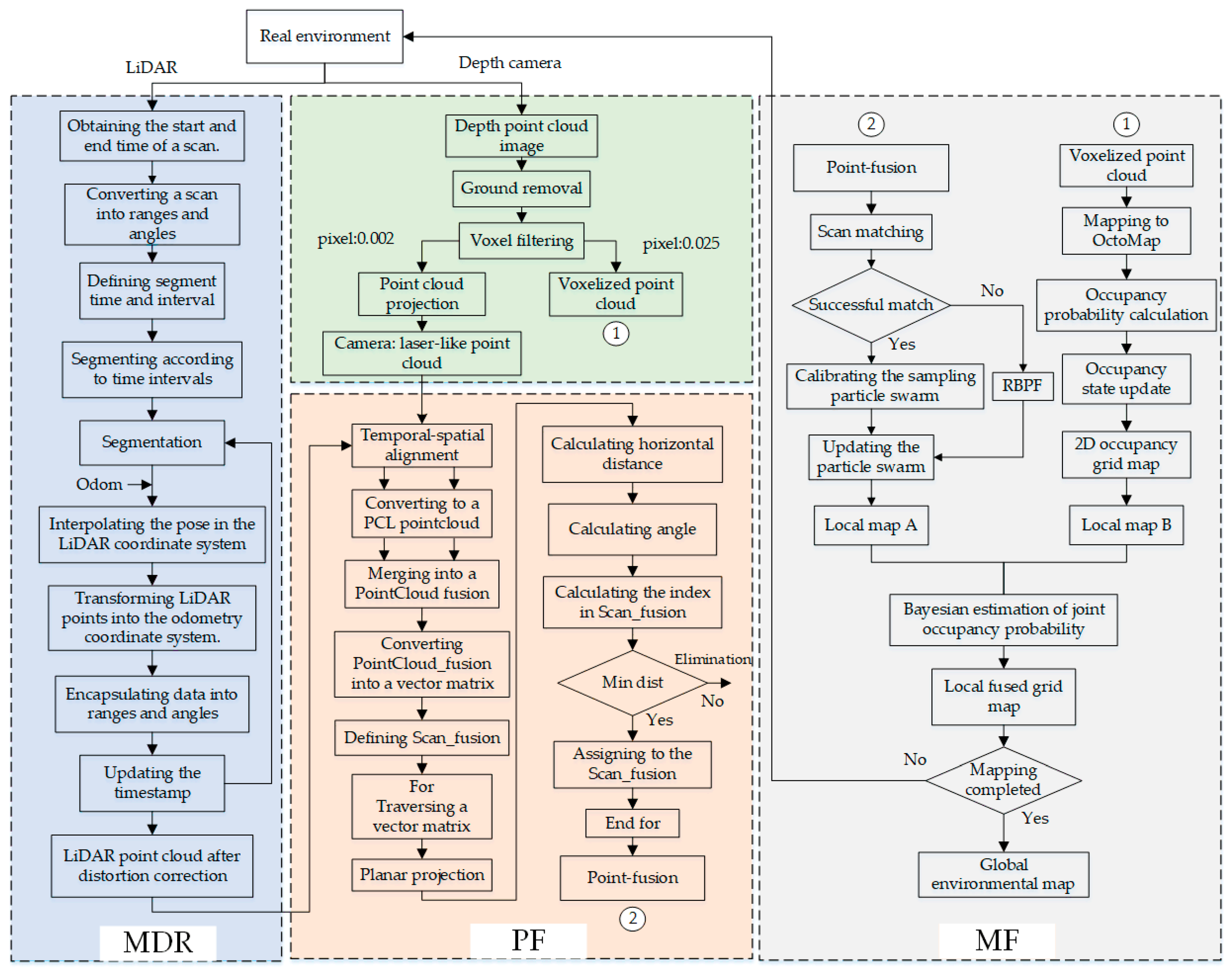
4.2. SLAM Map Construction Based on PF Method

The diverse fusion models of sensors have evolved into distributed, centralized and hybrid architectures. From the perspective of structural categories, they can be classified into strategy-level fusion, feature-level fusion and data-level fusion. Due to the high perception ability of the quadruped robot dog in obstacle detection, the requirements for the real-time performance of the structure and the robustness of the system are stringent. Moreover, there are differences in measurement angles, angular resolution, measurement radius, data frequency, and numbers of LiDAR point cloud data and laser-like point cloud data. Therefore, a distributed feature-level fusion was performed between the two. The pseudocode of the fusion algorithm (PF) is presented in Algorithm 1.

Algorithm 1 Data fusion algorithm for LiDAR point cloud and laser-like point cloud

Require: LiDAR point cloud $scan\_lidar$, laser-like point cloud $scan\_camera$.

Ensure: Fusion point cloud $scan\_fusion$.

1: Convert to PCL format $pointcloud\_lidar$ and $pointcloud\_camera$.

2: Merge to PCL Point Cloud $pointcloud\_fusion$.

3: Convert $pointcloud\_fusion$ to Vector matrix $matrix\_fusion$.

4: Define the max and min angles of $scan\_fusion$ as ${\theta }_{max}$ and ${\theta }_{min}$, Angle resolution $\theta$, Max and min scanning dist $r_{max}$ and $r_{min}$

5: $\mathbf{f}\mathbf{o}\mathbf{r}$ each ${\left(\begin{array}{ccc}{x}_k& y_k& z_k\end{array}\right)}^T\mathbf{d}\mathbf{o}$

6:          Project to the $xOy$ plane to obtain the projection point ${\left(\begin{array}{cc}{x}_k& y_k\end{array}\right)}^T$.

7:          $dist=\sqrt{x_k^2+y_k^2}$

8:          $if(dist<r_{min}||dist>r_{max})$

9:                   $continue$

10:          $endif$

11:          $angle=actan\left(y_k/x_k\right)$

12:          $if(angle<{\theta }_{min}||angle>{\theta }_{max})$

13:                   $continue$

14:          $endif$

15:          $index=(angle-{\theta }_{min})/\theta$

16:          $if(dist<{scan\_fusion}_{index})$

17:                   ${scan\_fusion}_{index}=dist$

18:          $endif$

19: $\mathbf{e}\mathbf{n}\mathbf{d}\mathbf{f}\mathbf{o}\mathbf{r}$

20: return $scan\_fusion$.

Firstly, the point cloud data of two sensors were transformed into PCL-formatted point cloud data in the world coordinate system. The PCL data were then used to merge the two point cloud data sets into a combined set of three-dimensional coordinate points that were represented as point cloud data $po\mathit{int}\_fusion$ in PCL format. These combined point cloud data were expressed in the form of a three-dimensional spatial vector matrix $matrix\_fusion$, enabling further processing and analysis.

Subsequently, the vector matrix was iterated, and each vector was projected onto a plane located 10 cm above the ground, as designed based on the step height of the robotic dog in this research. The horizontal distance (dist) from the projection point to the base coordinate system of the quadruped robot dog, as well as the angle $\left(anger\right)$ formed with the x-axis, were calculated. Then, based on $anger$, the current $index$ number (ind) of the projection point in the predefined fusion point cloud data array $scan\_fusion$ was determined. If a distance value for this $index$ already existed, the minimum distance value principle was applied to select the distance value, which was assigned to $scan\_fusio{n}_{index}$. This process was repeated for all of the column vectors in the vector matrix. Once all of the column vectors were traversed, the completed $scan\_fusio{n}_{index}$ array was returned, which represented the fusion point cloud data $scan\_fusion$.

The PF method was used to conduct obstacle detection experiments in different environmental types.

As shown in Figure 11a, multiple environments containing stacked typical obstacles are shown. These environments consist of rectangular paper boxes labeled as ① and ②, a sphere labeled as ③, another rectangular paper box labeled as ④, and a conical barrier with base labeled as ⑦; the two sensors obtained point clouds information with varying depth distances within their sensing range. For the sphere labeled as ⑥ and the cylindrical barrier labeled as ⑧, as well as the frame-type obstacle environment in Figure 10b which included benches, chairs and guardrails, the 2D LiDAR either failed to scan or captured minimal feature information. The PF method utilized the minimum distance principle to correctly extract the maximum contour information of the obstacle from the perspective of the LiDAR and camera detection after removing the invalid point cloud.

The PF method enhances the capability to detect obstacles in the forward direction, however it may not accurately construct an obstacle contour map. As shown in Figure 12, initially, the PF algorithm successfully detected a rectangular cardboard box obstacle (Figure 11, ④) and constructed a partial contour map. However, as the robot dog moved closer to the obstacle, the camera lost visibility of the cardboard box, and the scanning plane height of the LiDAR was higher than the box. Consequently, on the map, the rectangular box obstacle appeared as a sheet-like planar obstacle.

4.3. SLAM Map Construction Based on PMF Method

The point cloud data fusion method was enhanced to improve the ability to identify obstacle contour information and construct a more comprehensive environment map. The updated approach involved using the LiDAR point cloud after point cloud data fusion was used to construct a local map A, while employing the voxel point cloud to build a local map B. These two maps, A and B, were then subjected to inter-frame fusion using Bayesian estimation theory. It is important to note that both maps A and B needed to be generated with the same map resolution, in order to ensure accurate fusion results.

The pseudocode for the local grid map fusion based on Bayesian estimation is presented in Algorithm 2.

Algorithm 2 Bayesian Local Grid Map Fusion Algorithm

Require: Local grid maps $m_{1:N}$, parameters $\theta$.

Ensure: Global grid map $m_{global}$.

1: Initialize global grid map: $m_{global}=m_1$

2: $\mathbf{f}\mathbf{o}\mathbf{r}$ $n=2$ to $N$ do

3:   $\mathbf{f}\mathbf{o}\mathbf{r}$ each cell $i$ do

4:     Compute the occupancy probabilities $m_{global}\left(i\right)$ and $m_n\left(i\right)$ for cell $i$ in the global grid map and the $n$th local grid map, respectively.

5:     Compute the posterior probability $p\left(m_{global}\left(i\right)\right|m_n\left(i\right))$ using bayes-rule:         $p\left(m_{global}\left(i\right)\right|m_n\left(i\right))=\frac{p\left(m_n\right(i\left)\right|m_{global}\left(i\right)\left)p\right(m_{global}\left(i\right))}{p\left(m_n\right(i\left)\right)}$

6:     Update the occupancy probability in the global grid map using the posterior probability: $m_{global}\left(i\right)=p\left(m_{global}\right(i\left)\right|m_n\left(i\right))$

7:   $\mathbf{e}\mathbf{n}\mathbf{d}\mathbf{f}\mathbf{o}\mathbf{r}$

8: $\mathbf{e}\mathbf{n}\mathbf{d}\mathbf{f}\mathbf{o}\mathbf{r}$

9: Output the updated global grid map: $m_{global}$.

In the equation, $m_{global}\left(i\right)$ represents the occupancy probability of the ith grid in the global map, while $m_n\left(i\right)$ represents the occupancy probability of the ith grid in the nth local fusion map. When computing the posterior probability, the prior probability $p\left(m_{globao}\right(i\left)\right|m_n\left(i\right))$ needed to be used. When updating the global map, all of the grid’s posterior probabilities needed to be updated in order to obtain the correct probability values.

When the quadruped robot dog reached time $t(t\ge 0)$, the LiDAR or camera detected obstacles and updated the occupancy probability values of the corresponding grid cells. At this point, it was necessary to fuse the two probability estimates to obtain the occupancy probability $m_n\left(i\right)$ at time $t$. This process can be represented by Equation (5).

$$m_n\left(i\right)=\frac{{m_n}^L\left(i\right){m_n}^D\left(i\right)}{{m_n}^L\left(i\right){m_n}^D\left(i\right)+\left(1-{m_n}^L\left(i\right)\right)\left(1-{m_n}^D\left(i\right)\right)}$$

(5)

Equations ${m_n}^L\left(i\right)$ and ${m_n}^D\left(i\right)$ represent the occupancy probability estimates of the ith grid in the global map based on the LiDAR point cloud and the camera voxel point cloud in the nth local fusion map.

Equation $m_n\left(i\right)$ specifies the occupancy rules, as shown in

Table 2. Specific fusion rules.

	Camera Voxel Point Cloud	Occupancy	Vacancy	Unknown
Fused Point Clouds
Occupancy		⚫	⚫	⚫
Vacancy		⚫	◯	◯
Unknown		⚫	◯	⦿

Where ⚫ means occupancy, ◯ means vacancy and ⦿ means unknown.

.

As shown in Figure 13, the local grid map fusion method effectively addressed the problem of missing obstacle contour information shown in Figure 11, and correctly identified the rectangular cardboard box obstacle.

5. Overall Experiment

This chapter presents a comprehensive experiment divided into two parts. The first part involved conducting an obstacle detection experiment using three different methods: single LiDAR, the PF method, and the PMF method proposed in this study. The second part focused on a map construction experiment using the PMF method in complex laboratory scenarios, with and without MDR links. The experiments were designed to evaluate the performance and effectiveness of the proposed PMF method, in comparison to other methods, in detecting obstacles and constructing maps in different scenarios. The results of these experiments are presented and discussed in the following sections.

5.1. Sensor Information Fusion SLAM Map Construction Experiment

The experimental platform for the quadruped robot dog, as shown in Figure 14, consisted of several components. The 2D LiDAR (RPLiDAR_A3) was installed above the robot dog’s body, with a router and a protective plate placed underneath it. The router was powered by an external power bank. Additionally, the Intel RealSense D435 camera is installed at the front of the robot, facing downwards at a 15° angle. The relative positions of the LiDAR, camera, and the robot dog’s internal IMU sensors were determined through a multi-sensor joint calibration experiment.

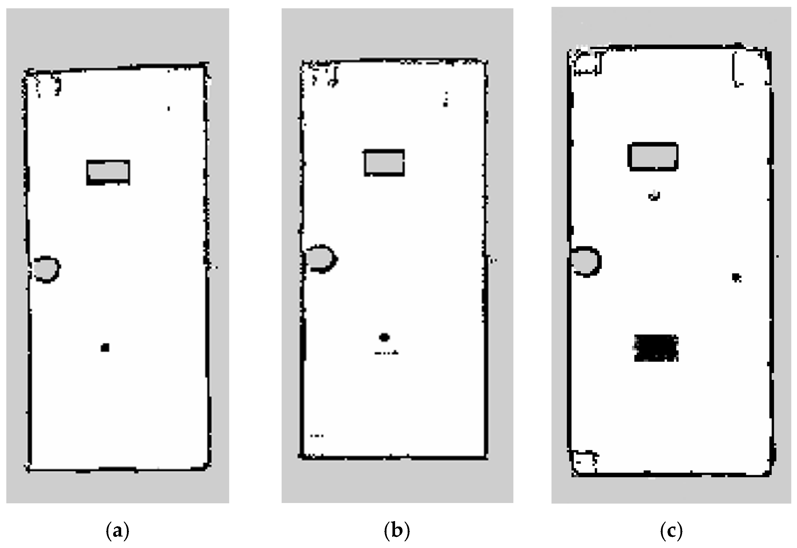
The purpose of this section was to conduct comparative experiments on three different methods, namely, single LiDAR, the PF method and the PMF method proposed in this study, in order to verify the effectiveness of the algorithm. The obstacle detection experiment environment consisted of a closed environment with an experimental table and a blue barrier, which included eight typical obstacles such as stools and chairs, as shown in Figure 15.

The experimental results, shown in Figure 16, revealed notable differences among the three methods for obstacle detection. In Figure 16a, the first method exhibited significant issues with missing obstacle information, resulting in only four obstacles being constructed in the map, with a detection success rate of 50%. Obstacles, such as single stools, chairs, footballs and blue cones below the height of the LiDAR installation, were not constructed in the map. In Figure 16b, the second method constructed a map with six obstacles and a detection success rate of 75%. However, the football and red cone obstacles were not constructed in the map, and construction of the red cone obstacle with the rectangular cardboard box as the base was inaccurate. In contrast, in Figure 16c, the third method utilized camera voxel point detection to obtain the three-dimensional contour information of the obstacles. and constructed a local grid map based on the LiDAR point cloud. The method also implemented frame-to-frame local map fusion with the grid mapping algorithm used in Figure 16b. Therefore, the constructed map was the most complete, with the outer contours of all eight objects accurately represented, and a detection success rate of 100%. Notably, in comparing the results shown in Figure 16a,b, the third method demonstrates a significant improvement in detection accuracy, with a 50% and 25% increase, respectively.

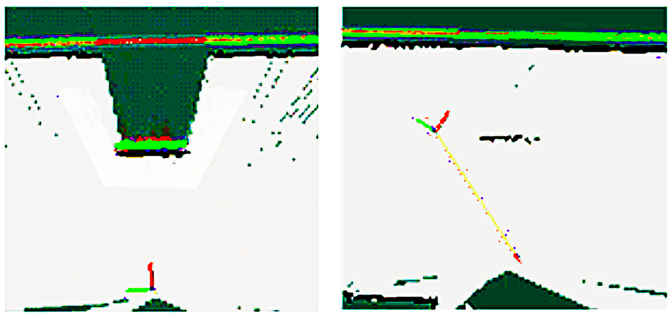
5.2. SLAM Experiments Performed before and after Motion Distortion

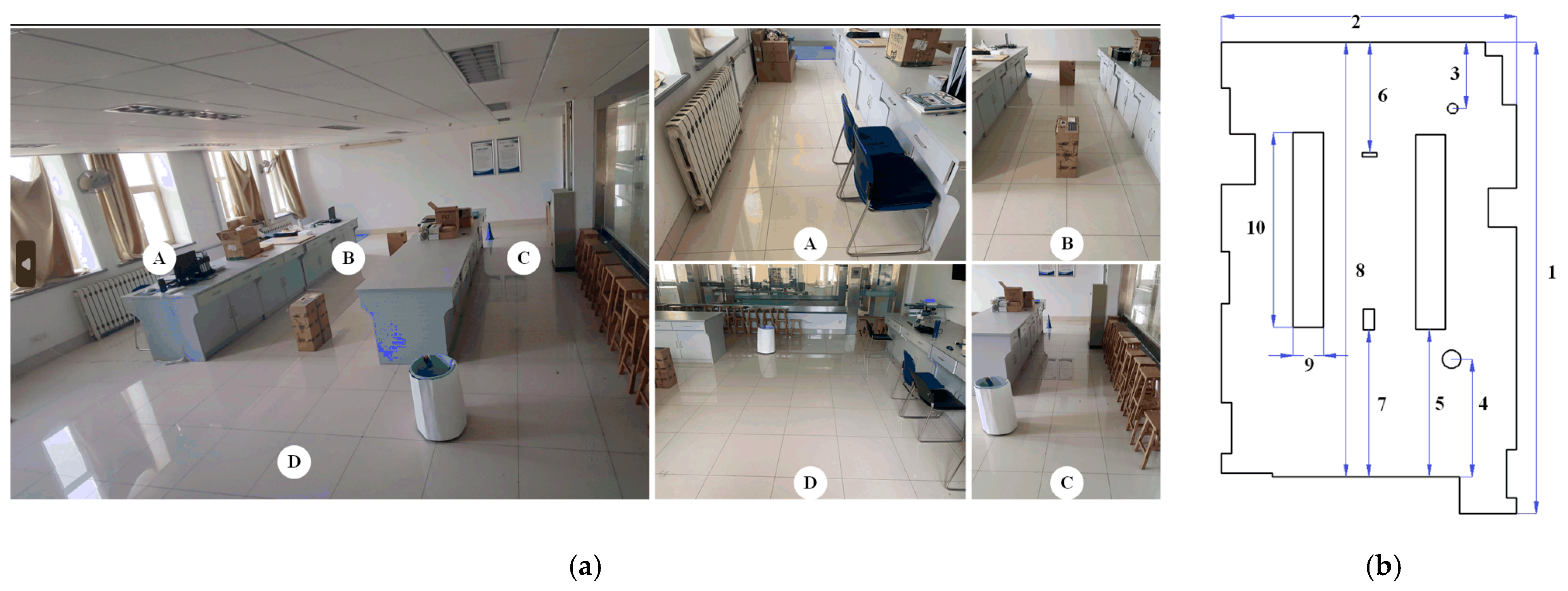
To assess the impact of mitigating motion distortion in the LiDAR point cloud on obstacle detection and SLAM fusion, an experiment was conducted in the environment shown in Figure 17.

The environment was divided into four distinct areas, labeled as A to D, with the experimental table located in the middle. Area A on the left side comprised obstacles such as cardboard boxes, radiators and chairs, while area B in the middle contained two rectangular cardboard box obstacles. Area C on the right side was populated with obstacles such as stools, rectangular distribution boxes and blue cone obstacles. Area D was an open environment with cylindrical barrels and four chairs as obstacles. Ten sets of key dimension data (outline size, location size of obstacles and overall size of the indoor environment) were selected, taking into consideration the overall size of the environment, the position and size of obstacles, as well as the contours of the obstacles.

The mapping of an open laboratory environment was performed with the use of a quadruped robot dog. Figure 18 illustrates the experimental outcomes, which revealed that the map generated through the proposed algorithm after motion distortion elimination exhibited significantly reduced drift and distortion issues compared to the map constructed by the fusion algorithm without distortion removal. In Figure 18a, stacking phenomena and angle distortion occurred at the map boundary marked as number ①. The contours of the three typical obstacles marked with number ② were distorted. The experimental table marked with number ③ was bent. There was a lot of noise and unclear contours in the bench area marked with number ④ and the chair area marked with number ⑤. However, after motion distortion removal, the results in Figure 18b demonstrate that no stacking phenomenon occurred in area ①, and the angle was right-angled. Additionally, the contours of the three typical obstacles marked with number ② were normal and complete. The experimental table in area ③ was not deformed. The contours of the bench and chair in areas ④ and ⑤ were continuous, and the noise was significantly reduced.

The laser rangefinder (accuracy ±1 mm) was used to measure 10 sets of marked feature sizes, and the average value was measured 10 times as the true value of the size. Then, the corresponding values of the dimensions were measured in the grid map using the measure tool in RVIZ. The measurements were also taken 10 times, and the average value was determined. Next, the relative errors between the measured values of the marked feature dimensions in the environment maps constructed by SLAM before and after removing motion distortion and the true values were calculated, and the error results are shown in Figure 18c. When using the PMF method for obstacle detection and mapping, the root mean square error (RMSE) value of the mapping without using the MDR algorithm reached 109 mm, while the RMSE value of the mapping using the MDR algorithm was 59 mm, improving the accuracy by about 45.9%.

The MDR algorithm introduced in this research can serve as an integral component of data preprocessing, applicable to both conventional 2D and 3D LiDAR SLAM techniques, as well as LiDAR–visual SLAM methodologies. By optimizing the LiDAR odometer, the precision of the SLAM algorithm was effectively enhanced. This study presented experimental evidence to validate the feasibility of employing various MDR techniques in 2D LiDAR SLAM (specifically the Gmapping algorithm), and compared the performance of LiDAR-camera fusion SLAM (utilizing the PMF algorithm) with or without the inclusion of the MDR link.

6. Conclusions

The proposed PMF obstacle detection method, which combines the PF algorithm and local grid map fusion algorithm based on Bayesian estimation, was demonstrated to enhance obstacle detection accuracy by 25% as compared to the PF method. To overcome the challenge of LiDAR point cloud motion distortion, the MDR algorithm was utilized to correct the distorted point cloud, followed by implementation of the PMF method for obstacle detection and mapping. The experimental results showed that employment of the MDR algorithm reduced the RMSE value to 59 mm, leading to a significant accuracy improvement of around 45.9% when compared to the method without the MDR algorithm (RMSE value of 109 mm).

References

1. Jiang, G.; Yin, L.; Jin, S.; Tian, C.; Ma, X.; Ou, Y. A simultaneous localization and mapping (SLAM) framework for 2.5 D map building based on low-cost LiDAR and vision fusion. Appl. Sci. 2019, 9, 2105. [Google Scholar] [CrossRef]
2. López, E.; García, S.; Barea, R.; Bergasa, L.M.; Molinos, E.J.; Arroyo, R.; Romera, E.; Pardo, S. A multi-sensorial simultaneous localization and mapping (SLAM) system for low-cost micro aerial vehicles in GPS-denied environments. Sensors 2017, 17, 802. [Google Scholar] [CrossRef]
3. Liu, J.Y. From big dog to spot mini: Evolution of boston powered quadruped robot. Robot Ind. 2018, 2, 109–116. [Google Scholar] [CrossRef]
4. Fankhauser, P.; Bloesch, M. Probabilistic Terrain Mapping for Mobile Robots With Uncertain Localization. IEEE Robot. Autom. Lett. 2018, 3, 3019–3026. [Google Scholar] [CrossRef]
5. Biswal, P.; Mohanty, P.K. Development of quadruped walking robots: A review. Ain Shams Eng. J. 2021, 12, 2017–2031. [Google Scholar] [CrossRef]
6. Kim, D.; Carballo, D.; Carlo, J.D.; Katz, B.; Bledt, G.; Lim, B.; Kim, S. Vision Aided Dynamic Exploration of Unstructured Terrain with a Small-Scale Quadruped Robot. In Proceedings of the 2020 IEEE International Conference on Robotics and Automation (ICRA), Paris, France, 31 May 2020–31 August 2020; pp. 2464–2470. [Google Scholar] [CrossRef]
7. Dudzik, T. Vision-Aided Planning for Robust Autonomous Navigation of Small-Scale Quadruped Robots. Ph.D. Thesis, Massachusetts Institute of Technology, Cambridge, MA, USA, 2020. Available online: https://hdl.handle.net/1721.1/129203 (accessed on 25 October 2022).
8. Barbosa, F.M.; Osório, F.S. Camera-Radar Perception for Autonomous Vehicles and ADAS: Concepts, Datasets and Metrics. arXiv 2023, arXiv:2303.04302. [Google Scholar] [CrossRef]
9. Wang, Y.; Zhu, R.; Wang, L.; Xu, Y.; Guo, D.; Gao, S. Improved VIDAR and machine learning-based road obstacle detection method. Array 2023, 18, 100283. [Google Scholar] [CrossRef]
10. Alfred, D.J.; Chandru, V.C.; Muthu, B.A.; Senthil, K.R.; Sivaparthipan, C.; Marin, C.E.M. Fully convolutional neural networks for LIDAR–camera fusion for pedestrian detection in autonomous vehicle. Multimed. Tools Appl. 2023, 1–24. [Google Scholar] [CrossRef]
11. Xizo, Y.F.; Huang, H.; Zheng, J.; Liu, R. Obstacle Detection for Robot Based on Kinect and 2D Lidar. J. Univ. Electron. Sci. Technol. China 2018, 47, 337–342. [Google Scholar] [CrossRef]
12. Liu, C.; Zhang, G.; Rong, Y.; Shao, W.; Meng, J.; Li, G.; Huang, Y. Hybrid metric-feature mapping based on camera and Lidar sensor fusion. Measurement 2023, 207, 112411. [Google Scholar] [CrossRef]
13. Shi, X.; Liu, T.; Han, X. Improved Iterative Closest Point (ICP) 3D point cloud registration algorithm based on point cloud filtering and adaptive fireworks for coarse registration. Int. J. Remote Sens. 2020, 41, 3197–3220. [Google Scholar] [CrossRef]
14. Hong, S.; Ko, H.; Kim, J. VICP: Velocity updating iterative closest point algorithm. In Proceedings of the 2010 IEEE International Conference on Robotics and Automation, Anchorage, AK, USA, 3–7 May 2010; pp. 1893–1898. [Google Scholar] [CrossRef]
15. Zheng, C.C.; Ke, F.Y.; Tang, Q.Q. Tightly coupled SLAM for laser inertial navigation based on graph optimization. Electron. Meas. Technol. 2023, 46, 35–42. [Google Scholar] [CrossRef]
16. Zhang, T.; Zhang, C.; Wei, H.Y. Design of Lidar Odemeter Integrating Lidar and IMU in Dynamic Environment. Navig. Position. Timing 2022, 9, 70–78. [Google Scholar] [CrossRef]
17. Zhang, F.; Zhai, W.F.; Zhang, Q.Y. Research on Motion Distortion Correction Algorithm Based on Laser SLAM. Ind. Control Comput. 2022, 35, 76–78. [Google Scholar]
18. Sun, T.; Feng, Y.T. Research on Gmapping Particle Filter SLAMBased on lmproved Particle Swarm Optimization. Ind. Control Comput. 2022, 35, 121–123+153. [Google Scholar]
19. Huang, R.; Zhang, S. High Adaptive Lidar Simultaneous Localization and Mapping. J. Univ. Electron. Sci. Technol. China 2021, 50, 52–58. [Google Scholar]
20. Yan, X.B.; Peng, D.G.; Qi, E.J. Research on Ground-Plane-Based Monocular Aided LiDAR SLAM. Acta Opt. Sin. 2020, 40, 173–183. Available online: https://kns.cnki.net/kcms/detail/31.1252.O4.20201211.1200.008.html (accessed on 25 October 2022).
21. Lin, H.Y.; Hsu, J.L. A sparse visual odometry technique based on pose adjustment with keyframe matching. IEEE Sens. J. 2020, 21, 11810–11821. [Google Scholar] [CrossRef]
22. Ghaffari Jadidi, M.; Clark, W.; Bloch, A.M.; Eustice, R.M.; Grizzle, J.W. Continuous Direct Sparse Visual Odometry from RGB-D Images. In Proceedings of the Robotics: Science and Systems 2019, Freiburg im Breisgau, Germany, 22–26 June 2019. [Google Scholar] [CrossRef]
23. Shao, H.; Zhao, Q.; Chen, B.; Liu, X.; Feng, Z. Analysis of Position and State Estimation of Quadruped Robot Dog Based on Invariant Extended Kalman Filter. Int. J. Robot. Autom. Technol. 2022, 9, 17–25. [Google Scholar] [CrossRef]
24. Zhao, Q.; Shao, H.; Yang, W.; Chen, B.; Feng, Z.; Teng, H.; Li, Q. A Sensor Fusion Algorithm: Improving State Estimation Accuracy for a Quadruped Robot Dog. In Proceedings of the 2022 IEEE International Conference on Robotics and Biomimetics (ROBIO), Jinghong, China, 5–9 December 2022; pp. 525–530. [Google Scholar] [CrossRef]
25. Zhang, Z. A Flexible New Technique for Camera Calibration. IEEE Trans. Pattern Anal. Mach. Intell. 2000, 22, 1330–1334. [Google Scholar] [CrossRef]
Figure 1. System framework diagram of the PMF algorithm.
Machines 11 00588 g001
Figure 2. Schematic diagram of sensor calibration.
Machines 11 00588 g002
Figure 3. Schematic diagram for the joint calibration of LiDAR and camera.
Machines 11 00588 g003
Figure 4. Joint calibration of LiDAR and depth camera. (a) Mapping and labeling of point cloud. (b) Calibration verification.
Machines 11 00588 g004
Figure 5. Schematic diagram of the time synchronization mechanism of different sensors.
Machines 11 00588 g005
Figure 6. Point cloud distortion phenomenon.
Machines 11 00588 g006
Figure 7. The position of odometer data interpolation during distortion correction.
Machines 11 00588 g007
Figure 8. Comparison of the effects before and after distortion correction during in-place rotation in a static environment for a quadruped robot dog. (a) Static environment. (b) Comparison of the effects before and after distortion correction during in-place rotation. 1. red-colored point cloud before distortion correction; 2. yellow-colored point cloud after distortion correction.
Machines 11 00588 g008
Figure 9. Comparison of three different methods to optimize the distortion point cloud after mapping effect. (a) Original distorted point cloud. (b) VICP method (Reference [14]). (c) IMU method (reference [18]). (d) Odom method (the method of this study).
Machines 11 00588 g009aMachines 11 00588 g009b
Figure 10. Comparison of the detection results of typical obstacles using LiDAR and camera. (a) Typical obstacles. (b) LiDAR point cloud (Gmapping). (c) Camera: depth point cloud. (d) Camera: laser-like point cloud (Gmapping). (e) Camera: voxel point cloud (OctoMap).
Machines 11 00588 g010
Figure 11. Complex environment with multiple obstacle types. (a) Various typical obstacles and overlapping situations. (b) Frame obstacles and superposition.
Machines 11 00588 g011
Figure 12. Obstacle detection based on the PF method.
Machines 11 00588 g012
Figure 13. Obstacle detection based on the PMF method.
Machines 11 00588 g013
Figure 14. Quadruped robot dog experimental platform. 1—Yobogo quadruped robot dog platform; 2—power bank; 3—router; 4—LiDAR protective plate; 5—2D LiDAR (RPLiDAR_A3); 6—fixture for securing the camera; 7—RealSense D435 depth camera.
Machines 11 00588 g014
Figure 15. Indoor corridor-like environment with both ends closed.
Machines 11 00588 g015
Figure 16. Comparison of obstacle detection results of different methods. (a) Obstacle detection and mapping results using only raw 2D LiDAR (RPLiDAR_A3) data. (b) Obstacle detection and mapping results based on the PF method (reference [11]). (c) Obstacle detection and mapping results based on PMF method (the method of this study).
Machines 11 00588 g016
Figure 17. Open laboratory environment for experiments. (a) Laboratory environment. (b) Ten sets of dimensions.
Machines 11 00588 g017
Figure 18. Comparison of PMF algorithm SLAM mapping results with and without MDR. (a) Without MDR. (b) With MDR. (c) Comparison of errors between 10 sets of dimensions and actual measured dimensions.
Machines 11 00588 g018