Enriched Finite Element Method Based on Interpolation Covers for Structural Dynamics Analysis

Abstract

This work proposes a novel enriched finite element method (E-FEM) for structural dynamics analysis. We developed the enriched 3-node triangular and 4-node tetrahedral displacement-based elements (T-elements). The standard linear shape functions of these T-elements were enriched using interpolation cover functions over each patch of elements. We also introduced and compared different orders of cover functions; higher-order functions obtained higher computational performance. Subsequently, the forced and free vibration analyses were performed on various typical numerical examples. The proposed enriched finite element method generated more precise numerical results and ensured faster convergence than the original linear elements.

1. Introduction

The recent use of FEM (finite element method) [1] has intensified in various engineering fields. Low-order three-node triangular elements [2] and four-node tetrahedral displacement-based elements [3] are commonly used in FEM due to its benefits of simple construction in complex structures. However, conventional low-order T-meshes still have defects in computational precision and sensitivity to mesh distortion. The “over-stiffness” properties of these T-meshes often yield poor computational outcomes (higher nature frequency) in the structural dynamics analysis. Significant research efforts are essential to improve the performance of these T-meshes.

Liu et al. [4] proposed a well-known strategy that incorporated gradient smoothing technology into the FEM. Based on alternative ways of constructing smoothing domains, the “over-stiffness” stiffness matrix of conventional FEM could be appropriately softened to a certain extent. Therefore, various S-FEMs [5,6,7,8,9] (Smoothed FEM) are proposed, including alpha FEM (α-FEM), beta FEM (β-FEM), face-based smoothed FEM (FS-FEM), node-based smoothed FEM (NS-FEM), edge-based smoothed FEM (ES-FEM), cell-based smoothed FEM (CS-FEM) [10], among other variations. In contrast with corresponding FEM, S-FEM yields more precise outcomes with higher convergence speed without increasing the relative computational cost [11,12,13,14]. The NS-FEM harbors an excessive softening effect on the system stiffness, resulting in unstable false shapes in structural dynamics analysis [11,12]. Unlike the “overly-stiff” FEM and the “overly-soft” NS-FEM model, the ES-FEM model has a closely exact stiffness. Besides, the ES-FEM has good mesh distortion adaptability [13,14,15,16,17]. For this reason, the ES-FEM is selected for comparison with the proposed approaches.

Another technique, the Enriched-FEM, was recently developed and used in various fields, including crack propagation, wave propagation, acoustic problems, multi-physical coupling, and solid mechanics. Bathe [18,19,20,21,22] and his colleagues first proposed this numerical approach to resolve issues in static analysis of solid mechanics and wave propagation. Wu [23] et al. adopted the E-FEM to efficiently minimize dispersion error at high frequencies and solve acoustic issues by applying the interpolation cover functions to improve the convergence rate and precision of solutions. The pertinent numerical findings indicate that the E-FEM may significantly minimize numerical dispersion error in wave propagation and considerably manufacture stable and more precise numerical solutions. Zhou [24] (2022) et al. utilized the E-FEM to analyze the dynamics of Magneto-electro-elastic (MEE) smart structures. The E-FEM outcomes used to examine the multi-physical coupling are consistent with the analytical analysis.

Furthermore, a variety of typical MEE-based specific examples have been used to reveal how efficiently the current E-FEM handles multi-physical coupling issues, unlike the conventional FEM. Li [25] and colleagues employed the supplementary interpolation cover functions, which are constructed using appropriate polynomial bases, to improve the performances of the traditional FEM at the same time handling 2D dynamic scenarios. As a result, the gradient field of the issue under examination can be more precisely described, and the initial linear approximation space of the conventional FEM can be considerably enriched [18,19,20,21,22,23,24,25,26,27]. In summary, E-FEM has extensive application prospects.

Herein, we propose a novel enriched finite element method with 3-node triangular and 4-node tetrahedral displacement-based elements for structural dynamic analysis. We also introduce and compare different orders of the cover functions using the standard FEM and recently developed ES-FEM. The enriched interpolation cover functions are constructed rather flexibly using different orders of the base functions. Numerical examples demonstrate that the proposed method provides more accurate numerical results and ensures faster convergence, unlike the original linear elements.

The rest of the article is organized as follows. The fundamental FEM theoretical formula and the E-FEM formula for structural dynamics analysis is thoroughly introduced in Section 2. The performance of the E-FEM is assessed using several numerical examples in Section 3 and Section 4. The conclusions are given in Section 5.

2. Formula of the E-FEM

Imagine that a typical finite element mesh has been created to solve a physical issue. The type of element and the mesh employed determine the precision of the sought-after solution. In order to improve the finite element procedure, we use the numerical manifold method’s earliest strategy and create tiny, overlapping sub-domains [28,29], where the finite elements in the supplied finite element mesh are the common parts of the sub-domains. Due to the interpolation covers utilized to cover each sub-domain, a higher-order interpolation of the desired solution is made feasible, increasing the accuracy of the results. Since our main goal is to enhance the performance of discretization utilizing these elements, we will now consider the 2D and 3D analytical situations using, respectively, the 3-node and 4-node low-order elements. Since they are trustworthy for both linear and nonlinear solutions, we use the traditional low-order finite elements; their fundamental flaw is the lack of precision in their results.

2.1. Theory of the E-FEM

The relevant issue domain is discretized using the common triangular elements with N nodes. And the interpolation for a scalar field function $d$ using the conventional FE approximation takes the following form.

$$d=\sum _{i=1}^N{N}_i{d}_i=\mathbf{N}\mathbf{d}$$

(1)

where $N_i$ denotes the piece-wise linear shape function and $d_i$ stands for the nodal field variable (see Figure 1a).

The traditional finite element (FE) mesh is still used in the current E-FEM. As seen in Figure 1a, the global elements connected to the node $i$ which is designated as the cover region ${\mathsf{\epsilon }}_i$ constitutes the support domain of the conventional linear nodal interpolation function in the standard FE interpolation. The following equation for the taken-in field variable $d$ at node $i$ improves the FE interpolation.

$$E_i^q\left[d\right]=\mathbf{L}{\left[\begin{array}{ccccc}{d}_i& a_{i1}& a_{i2}& a_{i3}& \cdots \end{array}\right]}^T$$

(2)

in which L refers to the degree $q$ polynomial bases that are applied over the cover region ${\mathsf{\epsilon }}_i$, $d_i$ denotes the conventional nodal variable, and ${\left[\begin{array}{cccc}{a}_{i1}& a_{i2}& a_{i3}& \cdots \end{array}\right]}^T$ is the extra unknowns connected to the interpolation cover functions.

$$\mathbf{L}=\left[\begin{array}{cccccccc}1& {\overline{x}}_i& {\overline{y}}_i& {\overline{x}}_i^2& {\overline{x}}_i{\overline{y}}_i& {\overline{y}}_i^2& \dots & {\overline{y}}_i^q\end{array}\right]$$

(3)

where ${\overline{x}}_i=x-x_i$ and ${\overline{y}}_i=y-y_i$ are the relative coordinate values $({\overline{x}}_i,{\overline{y}}_i)$ calculated from node $i$. (See Figure 1b)

Utilizing interpolation cover functions, we assign a group of full polynomial bases to each cover region in order to enrich the traditional FE interpolation for the solution of the variable $d$. Equation (2) can also be rewritten to provide a clear comparison with the common FE interpolation.

$$E_i^q\left[d\right]=d_i+\underset{\mathrm{additional}\mathrm{interpolation}\mathrm{cover}}{\underbrace{\left[\begin{array}{ccccccc}{\overline{x}}_i& {\overline{y}}_i& {\overline{x}}_i^2& {\overline{x}}_i{\overline{y}}_i& {\overline{y}}_i^2& \dots & {\overline{y}}_i^q\end{array}\right]\left[\begin{array}{c}{a}_{i1}\\ a_{i2}\\ \begin{array}{c}{a}_{i3}\\ ⋮\end{array}\\ a_{iq}\end{array}\right]}}$$

(4)

The interpolation scheme of E-FEM, which differs significantly from the current method from the traditional interpolation scheme of FEM, is shown to contain the additional interpolation cover in Equation (4).

Then, the global approximation for the regional variable $d$ can be obtained by

$$T{E}_i^q\left[d\right]=\sum _1^k\left(\sum _{i=1}^3{N}_i{E}_i^q\left[d\right]\right)=\sum _1^k\left(\sum _{i=1}^3{N}_i{d}_i+\sum _{i=1}^3{\mathit{H}}_i{\mathit{a}}_i\right)=\sum _1^k\left(\sum _{i=1}^3{N}_i{d}_i+\sum _{i=1}^3\sum _{j=1}^n{H}_{i,j}{a}_{i,j}\right)$$

(5)

where $k$ denotes the number of all nodes in $\mathsf{\Omega }$, $N_i$ denotes the linear interpolation for the nodes, $i$ and $j$ denote the additional degree of freedom in each node, and H is a matrix mixed with a q-order interpolation function.

$${\mathbf{H}}_i=N_i\left[\begin{array}{ccccccc}{\overline{x}}_i& {\overline{y}}_i& {\overline{x}}_i^2& {\overline{x}}_i{\overline{y}}_i& {\overline{y}}_i^2& \cdots & {\overline{y}}_i^q\end{array}\right]$$

(6)

The current E-FEM will become the standard FEM, as demonstrated by Equations (2) and (5) if the polynomial bases utilized only have the constant term 1 (i.e., q = 0). From this vantage point, it is possible to think of the current interpolation of E-FEM as including additional higher-order terms in addition to the traditional FE interpolation. The higher-order interpolation of solutions can be achieved using this technique. As a result, even with lower-order linear elements, a higher convergence rate and better numerical solution accuracy can be obtained.

In this study, the interpolation cover functions contain first-order polynomial bases $\left[1xy\right]$ $(q=1)$, second-order polynomial bases $\left[1xy{x}^2\right]$ $(q=2)$ and second order polynomial bases $\left[1xy{x}^{2}xy{y}^2\right]$ $(q=2)$, and three, four, and six additional DOFs are then introduced for each node for the 2D analysis, respectively. Then, four more DOFs will be inserted for each node for 3D analysis, and the interpolation cover functions will be first-order polynomial bases $\left[\begin{array}{cccc}1& x& y& z\end{array}\right]$ $(q=1)$.

Any order of polynomial bases may be utilized with interpolation cover functions and using high-order polynomial interpolation cover functions can also produce more accurate numerical results. However, the high order interpolation cover functions could increase the number of nodal unknowns and the computational cost.

For the 2D and 3D solid problem, the above-formulated interpolation of the E-FEM approach can be used to acquire the field variables $d$ and $v$ as follows:

$$d_h^k=\sum _{i=1}^6\left(N_i{d}_i+{\mathbf{H}}_i{\mathit{a}}_i^u\right),v_h^k=\sum _{i=1}^6\left(N_i{v}_i+{\mathbf{H}}_i{\mathit{a}}_i^v\right)$$

(7)

where ${\mathit{a}}_i^u$ and ${\mathit{a}}_i^v$ denote the vectors that hold additional unknowns, $u_i$ and $v_i$ denote the normal nodal unknowns as in the standard FEM.

Interpolation is enriched by using the unknowns arranged appropriately in the vector. Then $d_h^k$ and $v_h^k$ become

$$\left[\begin{array}{c}{d}_h^k\\ v_h^k\end{array}\right]=\left[\begin{array}{cccc}\mathbf{N}& \mathbf{H}& 0& 0\\ 0& 0& \mathbf{N}& \mathbf{H}\end{array}\right]\left[\begin{array}{c}\mathbf{d}\\ {\mathit{a}}_d\\ \mathbf{v}\\ {\mathit{a}}_v\end{array}\right]$$

(8)

where $\mathbf{H}$ denotes the supplementary interpolation cover function matrix, $\mathbf{N}$ stands for the conventional FEM interpolation function matrix, $\mathbf{d}$ and $\mathbf{v}$ are the typical nodal displacement vectors, and ${\mathit{a}}_v$ and ${\mathit{a}}_d$ stand for the additional unknown solution coefficient vectors.

Applying the common differentiation techniques to the derivatives of the displacement in the interpolation of E-FEM,

$$\left[\begin{array}{c}{d}_{h,x}^k\\ d_{h,y}^k\end{array}\right]=\left[\begin{array}{cc}{\mathbf{N}}_{,x}& {\mathbf{H}}_{,x}\\ {\mathbf{N}}_{,y}& {\mathbf{H}}_{,y}\end{array}\right]\left[\begin{array}{c}\mathbf{d}\\ {\mathit{a}}_d\end{array}\right],\left[\begin{array}{c}{v}_{h,x}^k\\ v_{h,y}^k\end{array}\right]=\left[\begin{array}{cc}{\mathbf{N}}_{,x}& {\mathbf{H}}_{,x}\\ {\mathbf{N}}_{,y}& {\mathbf{H}}_{,y}\end{array}\right]\left[\begin{array}{c}\mathbf{v}\\ {\mathit{a}}_v\end{array}\right]$$

(9)

where

$$\left[\begin{array}{cc}{\mathbf{N}}_{,x}& {\mathbf{H}}_{,x}\\ {\mathbf{N}}_{,y}& {\mathbf{H}}_{,y}\end{array}\right]={\mathbf{J}}^{-1}\left[\begin{array}{cc}{\mathbf{N}}_{,r}& {\mathbf{H}}_{,r}\\ {\mathbf{N}}_{,s}& {\mathbf{H}}_{,s}\end{array}\right]$$

(10)

where the usual FE formulation is used to generate the coordinate transformation between the natural coordinate ($r$, $s$, $t$) and the physical coordinate ($x$, $y$, $z$) (see Figure 1d), and $\mathbf{J}$ is the Jacobian matrix.

From the above formulas, the shape function matrix and the solid mechanical strain matrix B can be expressed as follows.

$${\mathbf{N}}_i=\left[\begin{array}{cccccccccccc}\mathbf{N}& \mathbf{N}x& \mathbf{N}y& \mathbf{N}{x}^2& \mathbf{N}xy& \mathbf{N}{y}^2& 0_{1\times 3}& 0_{1\times 3}& 0_{1\times 3}& 0_{1\times 3}& 0_{1\times 3}& 0_{1\times 3}\\ 0_{1\times 3}& 0_{1\times 3}& 0_{1\times 3}& 0_{1\times 3}& 0_{1\times 3}& 0_{1\times 3}& \mathbf{N}& \mathbf{N}x& \mathbf{N}y& \mathbf{N}{x}^2& \mathbf{N}xy& \mathbf{N}{y}^2\end{array}\right]$$

(11)

$$\mathbf{B}=\nabla {\mathbf{N}}_i=\left[\begin{array}{cccc}\partial \mathbf{N}/\partial x& \partial \mathbf{H}/\partial x& 0_{1\times 3}& 0_{1\times 15}\\ 0_{1\times 3}& 0_{1\times 15}& \partial \mathbf{N}/\partial y& \partial \mathbf{H}/\partial y\\ \partial \mathbf{N}/\partial y& \partial \mathbf{H}/\partial y& \partial \mathbf{N}/\partial x& \partial \mathbf{H}/\partial x\end{array}\right]$$

(12)

2.2. 3D Structural Element Construction Theory of the E-FEM

A 3D analysis domain Ω is discretized into several elements (taking the tetrahedral element as an example, the 2D element has less freedom than the 3D element). The basis function $e$ of [1 x y z] is first introduced at the node of the tetrahedral element in accordance with the characteristics of node displacement (Note: different types of basic functions can be selected, here only the simplest [1 x y z] is taken as an example). The node displacement of the element after introducing the basis function is shown in Figure 1c.

The node displacements are interpolated and described by:

$$\left\{\begin{array}{c}{u}_i=u_{i1}+{xu}_{i2}+y{u}_{i3}+{zu}_{i4}\\ v_i=v_{i1}+x{v}_{i2}+y{v}_{i3}+z{v}_{i4}\\ w_i=w_{i1}+x{w}_{i2}+y{w}_{i3}+z{w}_{i4}\end{array}\right\}$$

(13)

Then the displacement of any point in the element is redescribed:

$$\mathrm{d}=\sum _{i=1}^N{\mathbf{N}}_i{\mathbf{d}}_i={\mathbf{N}}_i\left\{\begin{array}{c}{u}_{i1}+{xu}_{i2}+y{u}_{i3}+{zu}_{i4}\\ v_{i1}+x{v}_{i2}+y{v}_{i3}+z{v}_{i4}\\ w_{i1}+x{w}_{i2}+y{w}_{i3}+z{w}_{i4}\end{array}\right\}={\mathbf{N}}_{\mathrm{E}-\mathrm{F}\mathrm{E}\mathrm{M}}{{\mathbf{d}}^{\mathrm{e}}}_{\mathrm{E}-\mathrm{F}\mathrm{E}\mathrm{M}}$$

(14)

where ${\mathbf{N}}_{\mathrm{E}-\mathrm{F}\mathrm{E}\mathrm{M}}$ denotes the new shape function matrix and ${{\mathbf{d}}^{\mathrm{e}}}_{\mathrm{E}-\mathrm{F}\mathrm{E}\mathrm{M}}$ denotes the node displacement vector after rearrangement, which is expressed as:

$$\{u_{11}{u}_{21}{u}_{31}{u}_{41}{u}_{12}{u}_{22}{u}_{32}{u}_{42}{u}_{13}{u}_{23}{u}_{33}{u}_{43}{u}_{14}{u}_{24}{u}_{34}{u}_{44}{v}_{11}{v}_{21}{v}_{31}{v}_{41}{v}_{12}{v}_{22}{v}_{32}$$

$$v_{42}{v}_{13}{v}_{23}{v}_{33}{v}_{43}{v}_{14}{v}_{24}{v}_{34}{v}_{44}{w}_{11}{w}_{21}{w}_{31}{w}_{41}{w}_{12}{w}_{22}{w}_{32}{w}_{42}{w}_{13}{w}_{23}{w}_{33}{w}_{43}{w}_{14}{w}_{24}{w}_{34}{w}_{44}{\}}^T$$

The basis function $\left[1xyz\right]$ is expressed as $E^T=\left[e_1{e}_2{e}_3{e}_4\right]$. It is possible to construct a new shape function matrix ${\mathbf{N}}_{\mathrm{E}-\mathrm{F}\mathrm{E}\mathrm{M}}$ from the rearranged node displacement vector ${{\mathbf{d}}^{\mathrm{e}}}_{\mathrm{E}-\mathrm{F}\mathrm{E}\mathrm{M}}$ as follows:

$${\mathbf{N}}_{\mathrm{E}-\mathrm{F}\mathrm{E}\mathrm{M}}=\mathbf{N}\mathbf{E}$$

(15)

where

$$\mathbf{N}=\left[\begin{array}{c}\begin{array}{cc}\begin{array}{cc}\begin{array}{ccc}{N}_1& 0& 0\end{array}& \begin{array}{ccc}{N}_2& 0& 0\end{array}\end{array}& \begin{array}{cc}\begin{array}{ccc}{N}_3& 0& 0\end{array}& \begin{array}{ccc}{N}_4& 0& 0\end{array}\end{array}\end{array}\\ \begin{array}{cc}\begin{array}{cc}\begin{array}{ccc}0& N_1& 0\end{array}& \begin{array}{ccc}0& N_2& 0\end{array}\end{array}& \begin{array}{cc}\begin{array}{ccc}0& N_3& 0\end{array}& \begin{array}{ccc}0& N_4& 0\end{array}\end{array}\end{array}\\ \begin{array}{cc}\begin{array}{cc}\begin{array}{ccc}0& 0& N_1\end{array}& \begin{array}{ccc}0& 0& N_2\end{array}\end{array}& \begin{array}{cc}\begin{array}{ccc}0& 0& N_3\end{array}& \begin{array}{ccc}0& 0& N_4\end{array}\end{array}\end{array}\end{array}\right]$$

(16)

$$\mathbf{E}={\left[\begin{array}{c}\begin{array}{cc}\begin{array}{cc}\begin{array}{ccc}{\mathrm{E}}_1& {\mathrm{E}}_0& {\mathrm{E}}_0\end{array}& \begin{array}{ccc}{\mathrm{E}}_2& {\mathrm{E}}_0& {\mathrm{E}}_0\end{array}\end{array}& \begin{array}{cc}\begin{array}{ccc}{\mathrm{E}}_3& {\mathrm{E}}_0& {\mathrm{E}}_0\end{array}& \begin{array}{ccc}{\mathrm{E}}_4& {\mathrm{E}}_0& {\mathrm{E}}_0\end{array}\end{array}\end{array}\\ \begin{array}{cc}\begin{array}{cc}\begin{array}{ccc}{\mathrm{E}}_0& {\mathrm{E}}_1& {\mathrm{E}}_0\end{array}& \begin{array}{ccc}{\mathrm{E}}_0& {\mathrm{E}}_2& {\mathrm{E}}_0\end{array}\end{array}& \begin{array}{cc}\begin{array}{ccc}{\mathrm{E}}_0& {\mathrm{E}}_3& {\mathrm{E}}_0\end{array}& \begin{array}{ccc}{\mathrm{E}}_0& {\mathrm{E}}_4& {\mathrm{E}}_0\end{array}\end{array}\end{array}\\ \begin{array}{cc}\begin{array}{cc}\begin{array}{ccc}{\mathrm{E}}_0& {\mathrm{E}}_0& {\mathrm{E}}_1\end{array}& \begin{array}{ccc}{\mathrm{E}}_0& {\mathrm{E}}_0& {\mathrm{E}}_2\end{array}\end{array}& \begin{array}{cc}\begin{array}{ccc}{\mathrm{E}}_0& {\mathrm{E}}_0& {\mathrm{E}}_3\end{array}& \begin{array}{ccc}{\mathrm{E}}_0& {\mathrm{E}}_0& {\mathrm{E}}_4\end{array}\end{array}\end{array}\end{array}\right]}^T$$

(17)

where

$${\mathrm{E}}_0=\left[\mathrm{0\; 0\; 0\; 0\; 0\; 0\; 0\; 0\; 0\; 0\; 0\; 0\; 0\; 0\; 0\; 0}\right]$$

(18)

$${\mathrm{E}}_1=\left[e_1\mathrm{0\; 0\; 0}{e}_2\mathrm{0\; 0\; 0}{e}_3\mathrm{0\; 0\; 0}{e}_4\mathrm{0\; 0\; 0}\right]$$

(19)

$${\mathrm{E}}_2=\left[0e_1\mathrm{0\; 0\; 0}{e}_2\mathrm{0\; 0\; 0}{e}_3\mathrm{0\; 0\; 0}{e}_4\mathrm{0\; 0}\right]$$

(20)

$${\mathrm{E}}_3=\left[\mathrm{0\; 0}{e}_1\mathrm{0\; 0\; 0}{e}_2\mathrm{0\; 0\; 0}{e}_3\mathrm{0\; 0\; 0}{e}_{4}0\right]$$

(21)

$${\mathrm{E}}_4=\left[\mathrm{0\; 0\; 0}{e}_1\mathrm{0\; 0\; 0}{e}_2\mathrm{0\; 0\; 0}{e}_3\mathrm{0\; 0\; 0}{e}_4\right]$$

(22)

After obtaining the shape function of the augmented FEM, the geometric matrix of the augmented FEM can be further written out:

$$\mathbf{B}=\mathbf{L}{\mathbf{N}}_{\mathrm{E}-\mathrm{F}\mathrm{E}\mathrm{M}}=\mathbf{L}\mathbf{N}\mathbf{E}$$

(23)

2.3. Dynamics Controlling Equations for Linear Elastic Solids

This section comprehensively introduces the discretization system equation and the standard FEM formula of the solid mechanics’ problem in the hypothetical bounded domain Ω. The standard Galerkin weak formula is given by:

$${\int }_{\mathsf{\Omega }}^{}{\left(▽\mathsf{\delta }\mathbf{d}\right)}^T\mathbf{D}▽\mathbf{d}d\mathsf{\Omega }={\int }_{\mathsf{\Omega }}^{}{\mathsf{\delta }\mathbf{d}}^T(\tilde{\mathbf{b}}-\mathsf{\rho }\ddot{\mathbf{d}}-\mathrm{c}\dot{\mathbf{d}})d\mathsf{\Omega }+{\int }_{{\mathsf{\Gamma }}_{\mathrm{N}}}^{}{\mathsf{\delta }\mathbf{d}}^T\mathrm{t}d\mathsf{\Gamma }$$

(24)

where ▽ is the differential operator, $\ddot{\mathbf{d}}$, $\dot{\mathbf{d}},$ and $\mathbf{d}$ denotes the acceleration, velocity vectors, and displacement vectors, respectively; the random virtual displacement vector is called δ$\mathbf{d}$, $\tilde{\mathbf{b}}$ stands for the body force vector, D denotes the constant matrix, ρ and c stand for the density and damping coefficients of the materials under consideration, and $\mathsf{\Gamma }$ denotes the prescribed traction vector on ${\mathsf{\Gamma }}_{\mathrm{N}}$ which denotes the natural boundary condition.

The matrix version of Equation (24) can be generated using the E-FEM interpolation technique by:

$$\mathbf{M}\ddot{\mathbf{d}}+\mathbf{C}\dot{\mathbf{d}}+\mathbf{K}\mathbf{d}=\mathbf{F}$$

(25)

$$\mathbf{M}=\sum _{i=1}^{n_e}{\int }_{{\mathsf{\Omega }}_i}^{}{\mathit{N}}_i^T\rho {\mathit{N}}_{i}d\mathsf{\Omega }$$

(26)

$$\mathbf{C}=\sum _{i=1}^{n_e}{\int }_{{\mathsf{\Omega }}_i}^{}{\mathit{N}}_i^{T}c{\mathit{N}}_{i}d\mathsf{\Omega }$$

(27)

$$\mathbf{K}=\sum _{i=1}^{n_e}{\int }_{{\mathsf{\Omega }}_i}^{}{\mathit{B}}_i^T\mathit{D}{\mathit{B}}_{i}d\mathsf{\Omega }$$

(28)

$$\mathbf{F}=\sum _{i=1}^{n_e}{\int }_{{\mathsf{\Omega }}_i}^{}{\mathit{N}}_i^T\overline{\mathit{b}}d\mathsf{\Omega }+\sum _{i=1}^{n_b}{\int }_{\overline{\mathsf{\tau }}}^{}{\mathit{N}}_i^T\mathit{t}d\mathsf{\tau }$$

(29)

$$\mathbf{D}=\frac{E}{1-v^2}\left[\begin{array}{ccc}1& v& 0\\ v& 1& 0\\ 0& 0& \frac{1-v}{2}\end{array}\right]$$

(30)

where M, $\mathbf{C}$, $\mathbf{K},$ and $\mathbf{D}$ denote the matrix of global mass, the damping effects, the global stiffness, and the material parameters, respectively, the global mesh’s total element count and the number of elements on the Neumann boundary are indicated by the characters $n_e$ and $n_b$, respectively, $\mathbf{F}$ denotes the nodal force vector, ${\mathit{B}}_i$ and ${\mathit{N}}_i$ denote the strain gradient matrix and the shape function matrix, respectively, ${\mathsf{\Omega }}_i$ stands for element $i$.

2.4. The Eigenvalue Problem of Free Vibration Analysis

If the damping effects ($\mathbf{C}=0$) are ignored, it is feasible to rewrite Equation (25) for free vibration analysis by

$$\mathbf{M}\ddot{\mathbf{d}}+\mathbf{K}\mathbf{d}=0$$

(31)

It is straightforward to determine that Equation (31) has the following basic solution,

$$\mathbf{d}=\overline{\mathbf{d}}\mathrm{e}\mathrm{x}\mathrm{p}\left(j\omega t\right)$$

(32)

where $\overline{\mathbf{d}}$ denotes the amplitude of displacement distributions, $j=\sqrt{-1}$, and $\omega$ denotes the angular frequency. We may obtain Equation (33) from Equations (31) and (32).

$$\mathbf{K}\overline{\mathbf{d}}-{{\omega }_p}^2\mathbf{M}\overline{\mathbf{d}}=0$$

(33)

The p-order natural frequency ${\omega }_p$ and the corresponding modal shape can be determined by adding up the eigenvectors and eigenvalues of Equation (33). The solution to the common eigenvalue problem is what Equation (33) indicates is the main goal of evaluating free vibration problems.

2.5. The Dynamic Problem of Forced Vibration Analysis

The second-order time-dependent dynamic issues, regulated by the matrix equation indicated in Equation (25), should be solved to perform forced vibration analysis [30,31]. Numerous other direct time integration strategies have been established in practice to solve structural dynamic issues. The widely used Newmark approach, an unconditionally stable direct time integration methodology, analyzes dynamic problems, and makes the following assumptions.

$$\left\{\begin{array}{c}{}^{t+∆t}\dot{\mathbf{d}}={}^t\dot{\mathbf{d}}+\left[\left(1-\beta \right){}^t\ddot{\mathbf{d}}+{}^{t+∆t}\ddot{\mathbf{d}}\beta \right]∆t\\ {}^{t+∆t}\mathbf{d}={}^t\mathbf{d}+{}^t\dot{\mathbf{d}}∆t+\left[\left(\frac{1}{2}-\alpha \right){}^t\ddot{\mathbf{d}}+{}^{t+∆t}\ddot{\mathbf{d}}\alpha \right]∆t^2\end{array}\right.$$

(34)

where $∆t$ is the time step for the temporal integration and α and δ are the unknown coefficients associated with the accuracy of the integration.

Additionally, the equilibrium equation at time $t+∆t$ following should also be utilized,

$$\mathbf{C}^{t+∆t}\dot{\mathbf{d}}+\mathbf{M}^{t+∆t}\ddot{\mathbf{d}}+\mathbf{K}^{t+∆t}\mathbf{d}=\mathbf{F}$$

(35)

These two parameters are utilized in this work since they will not add any numerical dampening effects to the result when $\beta =1/2$ and $\mathsf{\alpha }=1/4$. Combining Equations (25) and (34), when $t+∆t$ time arrives, we can acquire,

$$\left(\frac{4}{\mathsf{\Delta }{\mathrm{t}}^2}\mathbf{M}+\frac{2}{\mathsf{\Delta }\mathrm{t}}\mathbf{C}+\mathbf{K}\right){}^{t+∆t}\mathbf{d}=\mathbf{M}\left(\frac{4}{\mathsf{\Delta }{\mathrm{t}}^2}{}^t\mathbf{d}+\frac{4}{\mathsf{\Delta }\mathrm{t}}{}^t\dot{\mathbf{d}}+{}^t\ddot{\mathbf{d}}\right)+\mathbf{C}\left(\frac{2}{\mathsf{\Delta }\mathrm{t}}{}^t\mathbf{d}+{}^t\dot{\mathbf{d}}\right)$$

(36)

After that, the whole numerical solution can be obtained by repeatedly applying Equations (34) and (35).

3. Analysis of 2D Examples

First, we used 2D examples to evaluate and analyze the numerical convergence and accuracy of E-FEM.

3.1. The Cantilever Beam

Unless otherwise stated, the global standard unit system is the foundation for all physical units used in the current work. The numerical experiment of 2D free vibration analysis was performed with a cantilever beam model (see Figure 2). We studied various behaviors of E-FEM elements of a 2D cantilever beam with height D and length L. The inputs used in the calculation included: Young’s modulus $E=2.1\times {10}^4\mathrm{k}\mathrm{g}\mathrm{f}/{\mathrm{m}\mathrm{m}}^2$, thickness $t=1\mathrm{m}\mathrm{m}$, Poisson’s ratio $v$ = 0.3, $\mathrm{D}=10\mathrm{m}\mathrm{m}$, $L=100\mathrm{m}\mathrm{m}$, mass density $\rho =8.0\times {10}^{-10}\mathrm{k}\mathrm{g}\mathrm{f}{\mathrm{s}}^2/{\mathrm{m}\mathrm{m}}^4$. This was obtained by dividing the cantilever beam of Figure 2 into three types of meshes with different precision in Figure 3. Liu and Nguyen-Thoi, and Nagashima have already examined this issue using NS-FEM and ES-FEM [32,33]; Liu and Nguyen-Thoi used the node-by-node meshless (NBNM) approach; Liu and Gu utilized the Gaussian radial function [34] and local radial point interpolation method (LRPIM) with multi-quadrics (MQ) radial function.

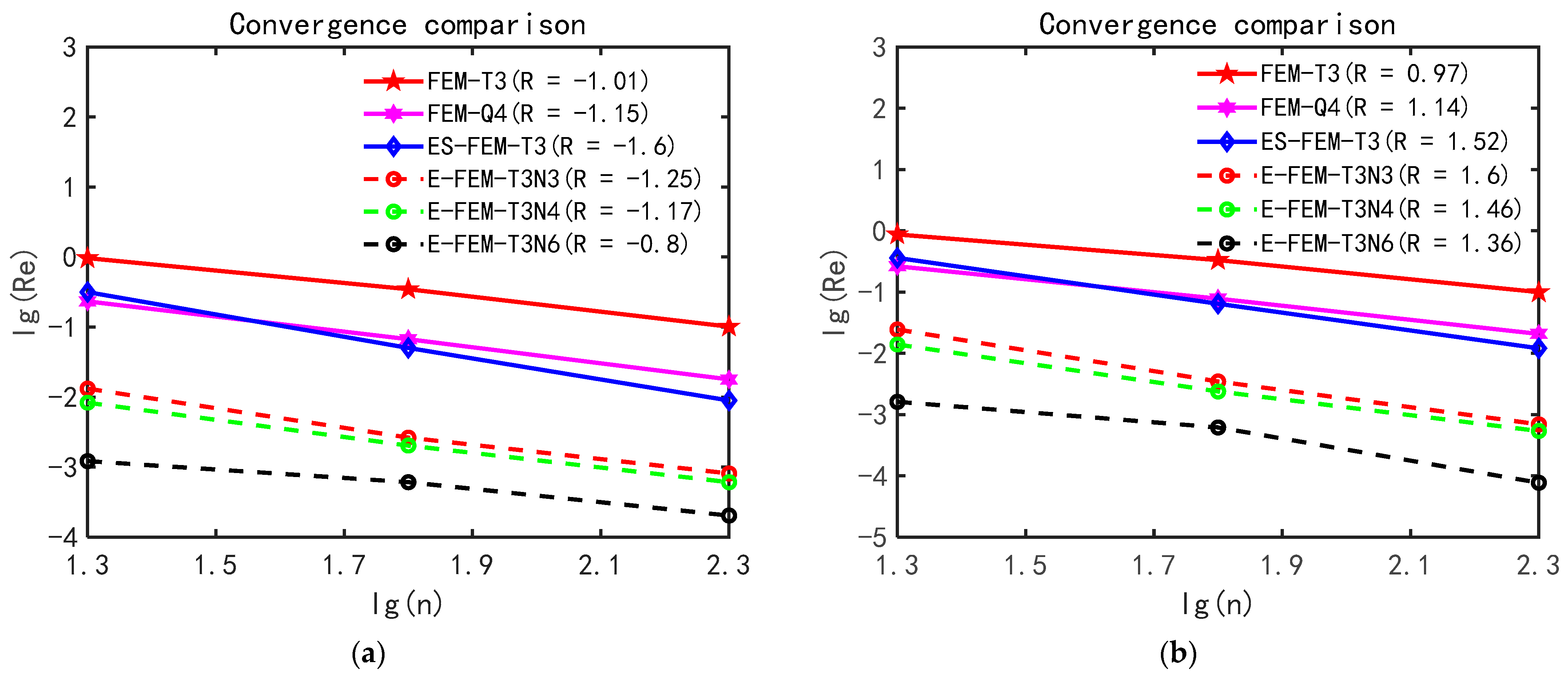
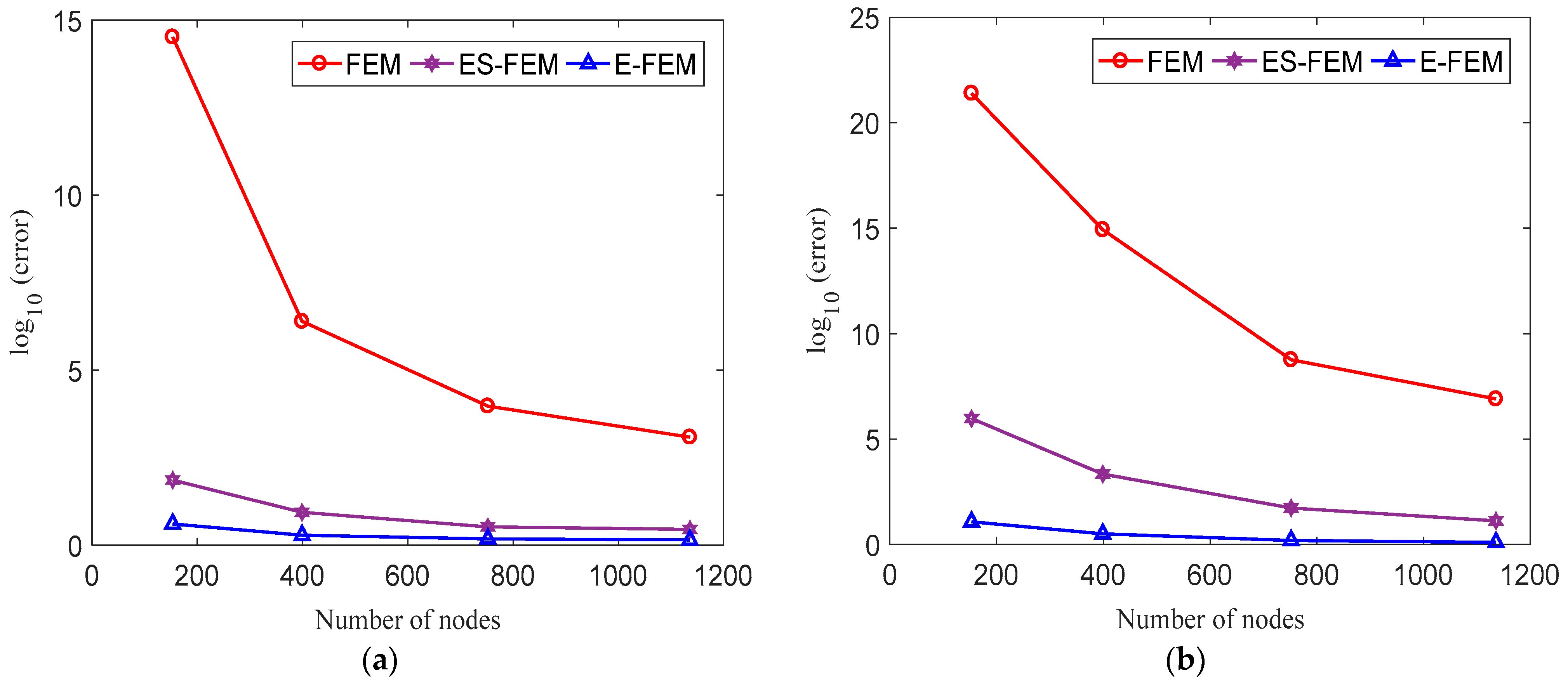
3.1.1. Convergence Study

FEM-T3, E-FEM-T3, E-FEM-T3N4, and E-FEM-T3N6 were used in MATLAB to evaluate and calculate Mesh a, b, and c. Retrieving the frequencies of

Table 1. Results of frequencies (Hz) of grid A ($10\times 1$) (22 nodes, 20 elements).

Order	FEM-T3	FEM-Q4	ES-FEM-T3	E-FEM- T3N3	E-FEM- T3N4	E-FEM- T3N6	References
$f_1$	1708	992	1048	826	826	823	822
$f_2$	9689	5791	6018	4997	4973	4938	4932
$f_3$	12,908	12,834	12,833	12,834	12,833	12,827	12,824
$f_4$	24,331	14,830	15,177	13,311	13,174	13,014	12,993
$f_5$	39,193	26,183	26,362	24,523	24,111	23,670	23,611
$f_6$	42,944	38,140	37,724	37,946	37,051	36,149	36,010
$f_7$	64,559	38,824	38,559	38,482	38,473	38,453	38,444
$f_8$	67,691	51,924	50,349	53,047	51,413	49,865	49,578
$f_9$	90,810	62,345	60,827	64,059	64,032	63,990	63,913
$f_{10}$	98,302	64,846	61,520	69,457	66,800	64,440	63,975

,

Table 2. Results of frequencies (Hz) grid B ($20\times 2$) (63 nodes, 80 elements).

Order	FEM-T3	FEM-Q4	ES-FEM-T3	E-FEM-T3N3	E-FEM-T3N4	E-FEM-T3N6	References
$f_1$	1120	870	853	824	824	823	822
$f_2$	6644	5199	5078	4945	4942	4935	4932
$f_3$	12,852	12,830	12,828	12,828	12,827	12,825	12,824
$f_4$	17,307	13,640	13,246	13,038	13,024	13,001	12,993
$f_5$	31,173	24,685	23,783	23,729	23,687	23,629	23,611
$f_6$	38,686	37,477	35,784	36,259	36,165	36,041	36,010
$f_7$	47,342	38,378	38,298	38,455	38,454	38,448	38,444
$f_8$	64,769	51,322	48,533	50,037	49,858	49,628	49,578
$f_9$	65,365	63,585	61,527	63,996	63,991	63,975	63,913
$f_{10}$	84,519	65,731	63,182	64,678	64,373	63,992	63,975

and

Table 3. Results of frequencies (Hz) of grid C ($40\times 4$) (205 nodes, 320 elements).

Order	FEM-T3	FEM-Q4	ES-FEM-T3	E-FEM-T3N3	E-FEM-T3N4	E-FEM-T3N6	Reference
$f_1$	907	835	827	823	823	823	822
$f_2$	5431	5004	4950	4936	4935	4933	4932
$f_3$	12,834	12,827	12,826	12,825	12,825	12,824	12,824
$f_4$	14,286	13,174	13,006	13,002	13,000	12,994	12,993
$f_5$	25,949	23,926	23,554	23,631	23,626	23,614	23,611
$f_6$	38,511	36,462	35,778	36,046	36,035	36,014	36,010
$f_7$	39,612	38,431	38,408	38,448	38,447	38,445	38,444
$f_8$	54,647	50,150	49,029	49,638	49,619	49,584	49,578
$f_9$	64,236	63,883	62,867	63,980	63,969	63,919	63,913
$f_{10}$	70,685	64,561	63,774	64,007	63,985	63,976	63,975

was possible in ten different modes. The following is the expression for the relative error of natural frequency, where n refers to the number of nodes, which is used to assess precision and convergence.

$$R_e=\left|\frac{f_{num}-f_{ref}}{f_{ref}}\right|\times 100\%$$

(37)

where the superscript “ref” means reference solution and the superscript “num” means numerical solution.

Then, using $lg\left(n\right)$ as the abscissa and $R_e$ as the ordinate, taking the former two modes as examples, the relative error diagram of Figure 4 was obtained by comparing it with a reference value. Table 1, Table 2 and Table 3 present a list of the frequencies calculated for the three meshes.

Figure 4 displays the natural frequency error of the second and fourth modes. In addition, the convergence comparison concluding the FEM-T3, E-FEM-T3N3, E-FEM-T3N4, E-FEM-T3N6, ES-FEM-T3, and FEM-Q4 are displayed in Figure 5. Based on the simulation results, the second and fourth natural frequencies of E-FEM-T3, which include E-FEM-T3N3, E-FEM-T3N4, and E-FEM-T3N6, have a considerably smaller error and a significant accuracy than FEM-Q4, E-FEM, and ES-FEM. Compared to other methods for the same mesh without adding new nodes, the performance of E-FEM in terms of calculation accuracy is rolled over with an inaccuracy of only about a thousandth. Additionally, under the same node and grid density, the accuracy of the E-FEM algorithm increases with increasing order q or the number of terms N.

Figure 6 displays the first to tenth eigenmodes concluded using the E-FEM element of Mesh. These model diagrams are superior compared to ES-FEM [13,17,35].

3.1.2. Grid Distortion Sensitivity Study

We give the distorted element mesh in Figure 7, and d is the distorted displacement.

We can learn the following information by comparing relative errors of calculated frequencies, as shown in Figure 8 and

Table 4. Grid distortion sensitivity calculation results.

$2\mathit{d}/\mathit{b}$	FEM-T3	FEM-Q4	ES-FEM-T3	E-FEM- T3N3	E-FEM- T3N4	E-FEM- T3N6	References
0.000	4256	2623	2947	870	851	829.0	822
0.025	4413	2710	3163	875	853	829.5	822
0.050	4560	2889	3413	890	856	829.7	822
0.075	4674	3052	3614	913	860	830.0	822
0.100	4762	3169	3758	939	863	830.3	822
0.150	4902	3296	3937	983	870	830.8	822
0.200	5023	3352	4052	1007	877	831.5	822
0.250	5137	3386	4141	1018	884	832.3	822
0.300	5248	3417	4221	1024	892	833.0	822
0.400	5468	3498	4366	1030	909	834.0	822
0.500	5688	3617	4499	1033	928	835.0	822
0.600	5910	3776	4623	1035	946	835.7	822
0.700	6134	3984	4741	1037	963	836.4	822
0.800	6361	4252	4856	1039	978	837.2	822
0.900	6591	4617	4968	1040	992	841.2	822

. First, as deformation increases, the numerical error of the E-FEM-T3 does not vary significantly, whereas the numerical error of the FEM-T3 and FEM-Q4 varies. Secondly, the E-FEM-T3 curve is the lowest, with the smallest relative error. Thirdly, the error curves formed by FEM-T3 and FEM-Q4 follow a similar trend, with the error increasing when distortion parameters are increased. Fourthly, the curves of E-FEM-T3 are close to parallel lines, indicating that grid deformation has little effect on the error [36,37].

Figure 9 shows the two distorted grids established to assess the effect of grid quality on relative error. Three methods, FEM-T3, ES-FEM-T3, and E-FEM-T3, are shown in

Table 5. Computed frequencies (Hz) of distorted grids in Figure 9b.

Order	FEM-T3	ES-FEM-T3	E-FEM- T3N3	E-FEM- T3N4	E-FEM- T3N6	References
$f_1$	1376	947	825	824	823	822
$f_2$	8554	5663	4960	4946	4936	4932
$f_3$	12,870	12,827	12,828	12,828	12,825	12,824
$f_4$	21,883	14,726	13,112	13,036	13,004	12,993
$f_5$	38,777	27,242	23,975	23,715	23,637	23,611
$f_6$	40,231	38,194	36,927	36,214	36,059	36,010
$f_7$	62,931	39,798	38,458	38,456	38,449	38,444
$f_8$	67,377	54,754	51,329	49,958	49,668	49,578
$f_9$	86,597	62,901	64,010	63,996	63,982	63,913
$f_{10}$	94,872	72,378	66,640	64,569	64,080	63,975

and

Table 6. Computed frequencies (Hz) of distorted grids in Figure 9c.

Order	FEM-T3	ES-FEM-T3	E-FEM- T3N3	E-FEM- T3N4	E-FEM- T3N6	References
$f_1$	1584	1029	825	824	822	822
$f_2$	9522	6227	4978	4944	4936	4932
$f_3$	12,887	12,826	12,828	12,828	12,825	12,824
$f_4$	24,124	15,611	13,283	13,030	13,002	12,993
$f_5$	39,120	29,557	24,373	23,704	23,635	23,611
$f_6$	47,170	38,019	37,259	36,235	36,078	36,010
$f_7$	67,566	46,072	38,460	38,455	38,448	38,444
$f_8$	74,501	61,371	53,065	49,995	49,708	49,578
$f_9$	97,634	63,573	64,021	63,993	63,981	63,913
$f_{10}$	102,709	76,854	70,025	64,674	64,180	63,975

. The enriched K-matrix and M-matrix of proposed E-FEM-T3 often yield better accuracy than that of FEM-T3 and Quad 4. Even for distorted grids, good results can be obtained using E-FEM-T3 elements. This is a significant benefit of the E-FEM-T3 method. The result is valuable for the practical application of E-FEM-T3. Unlike the E-FEM method, E-FEM-T3 can yield better results; however, additional nodes are necessary to increase the stiffness matrix.

In practical engineering problems, grid distortion will also have a certain impact on calculation accuracy. The next sections further explore the capacity of the E-FEM-T3 to resist grid distortion.

Figure 10 reveals a similar number of nodes in both uniform and distorted meshes, in which a higher degree of irregularity causes a more distorted mesh. Table 5 and Table 6 show the top 10 natural frequency outcomes from various elements using two distorted meshes. The tables also include matching computation results from the uniform mesh and reference solutions. The findings indicate that using the distorted mesh pattern will significantly reduce the precision of the standard linear elements (FEM-T3 and FEM-Q4). Although the estimated numerical solutions are excellent when using the deformed mesh, the present E-FEM-T3 method performs the best among all the factors considered. With a larger irregularity indication, these conclusions become increasingly more obvious. The E-FEM performs significantly better than the conventional FEM and ES-FEM. This indicates that, unlike other elements, the current E-FEM-T3 has a larger tolerance for mesh distortion.

Figure 11 shows the related E-FEM and FEM element solution times, and the relative imprecision of the two natural frequencies. At the second natural frequency, the E-FEM-T3N3 element converges at a rate of 0.82 slower than the FEM. Regarding the convergence rate at the fourth natural frequency, the FEM element performs better than the E-FEM element, standing at 1.71. As shown, the convergence rate of error relative to computation time for the three E-FEM algorithms reduces as N increases. The accuracy of distorted and standard meshes can be improved using a similar mesh to the E-FEM-T3 element. The E-FEM-T3 increases the computation time by increasing the bandwidth of the total stiffness matrix. Therefore, there is a significant urgency to strike a good balance between accuracy and computational speed for the E-FEM-T3 approach.

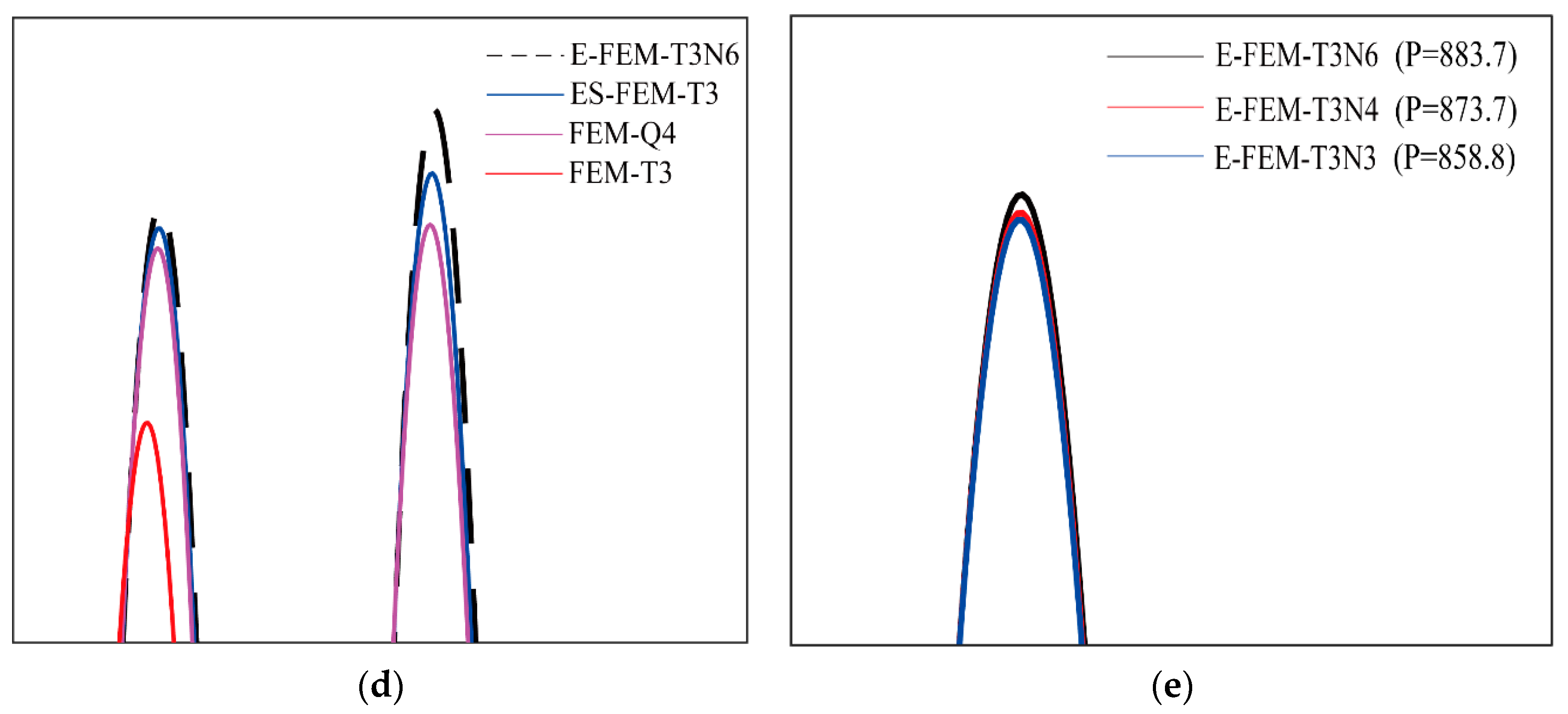
3.1.3. Forced Vibration Study

The E-FEM was used to investigate a benchmark cantilever beam problem using the Newmark method for time stepping. A tip harmonic loading in the y-direction, $f\left(t\right)=\cos {\omega }_{f}t$, was applied to the beam. The numerical parameters used to consider the plane strain problem included: $E=0.1$, $H=1.0$, $L=4.0$, $v=0.3$, $\mathsf{\alpha }=0.005$, $\mathsf{\beta }=0.272$, $t$ = 1.0. The model comprised 100 units and 126 nodes, computing with an amplitude time step of $∆t=1$. By analyzing the performance of E-FEM-T3, FEM-Q4, ES-FEM-T3, and FEM-T3 in this model, the vibration periods of E-FEM-T3 and FEM-Q4, ES-FEM-T3 and FEM-T3 were highly consistent (Figure 12a). Furtherly the amplitude of E-FEM-T3 was larger than that of ES-FEM-T3, that of ES-FEM-T3 was larger than that of FEM-Q4, and that of FEM-Q4 was larger than that of FEM-T3. The peak of each curve reached FEM-T3 (526.4), FEM-Q4 (809.6), ES-FEM-T3 (843.8), E-FEM-T3N3 (858.8), E-FEM-T3N4 (873.7) and E-FEM-T3N6 (883.7). The larger the amplitude, the softer the model. Therefore, the model accuracy of FEM-Q4 is higher than that of FEM-T3, with better convergence efficiency. Similarly, E-FEM-T3 achieves higher model accuracy and better convergence efficiency [38,39].

3.2. A Shear Wall

Figure 13 illustrates how Brabbia et al. solved a straightforward model of a four-opening shear wall with an assumed plane stress condition using the boundary element approach. In Figure 14, 559 uniformed nodes remedied the issue. Young’s modulus $E=1\times {10}^3$, Poisson’s ratio $v=0.2$, thickness $t=1$, mass density $\rho =1$, and these were the pertinent values. Figure 14 presents the grid computed with 952 cells and 559 nodes. As shown in

Table 7. Natural frequencies (Hz) of a shear wall.

Order	FEM-T3	FEM-Q4	ES-FEM-T3	E-FEM- T3N3	E-FEM- T3N4	E-FEM- T3N6	References
$f_1$	0.1081	0.1044	0.1032	0.1021	0.1019	0.1014	0.1011
$f_2$	0.3681	0.3580	0.3553	0.3520	0.3515	0.3504	0.3497
$f_3$	0.3855	0.3839	0.3836	0.3830	0.3828	0.3826	0.3825
$f_4$	0.6312	0.6029	0.5916	0.5839	0.5823	0.5788	0.5767
$f_5$	0.8094	0.7773	0.7677	0.7587	0.7579	0.7549	0.7532
$f_6$	0.9503	0.9275	0.9214	0.9135	0.9119	0.9103	0.9094
$f_7$	1.0352	1.0061	0.9983	0.9898	0.9882	0.9865	0.9857
$f_8$	1.1459	1.1247	1.1158	1.1106	1.1045	1.1021	1.1007
$f_9$	1.2045	1.1673	1.1552	1.1450	1.1434	1.1404	1.1389
$f_{10}$	1.2276	1.1944	1.1844	1.1760	1.1750	1.1720	1.1724

, the E-FEM was used to calculate the natural frequencies of the first 10 modes. The E-FEM-T3 results are typically the ones closest to the reference solution since the generated natural frequencies are significantly bigger than the FEM-T3, which is excessively stiff. Considering that the natural frequencies are a reliable sign for determining the stiffness of a model, the results mentioned above verify that the E-FEM-T3 has extremely close-to-exact stiffness.

We give the first 10 vibration modes of the shared wall computed using E-FEM in Figure 15. It is obvious that the proposed E-FEM indeed behaves very well in predicting the mode shape in free vibration analysis.

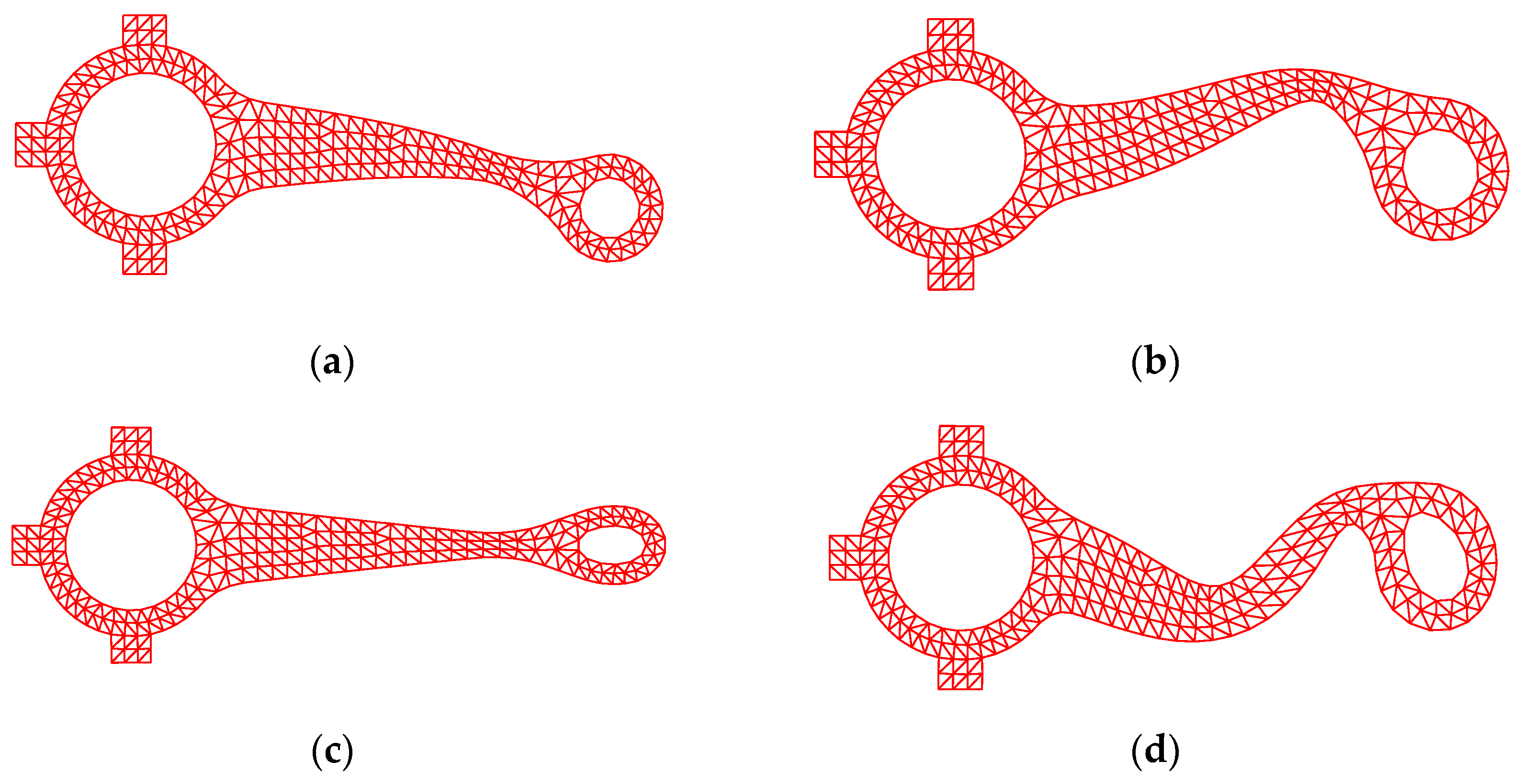
3.3. A Connecting Rod

We established a simple connecting rod with a large and small opening, as shown in Figure 16. The free vibration of the rod was analyzed under the assumption of plane stress state; the relevant calculation parameters included mass density $\rho =7800$ kg/m³, Young’s modulus $\mathrm{E}=10$ GPa, and Poisson’s ratio $v$ = 0.3. Two set directions existed on the left inner circle of the rod. As shown in

Table 8. First 10 natural frequencies (HZ) of a connecting rod.

Order	FEM-T3	FEM-Q4	ES-FEM-T3	E-FEM- T3N3	E-FEM- T3N4	E-FEM- T3N6	References
$f_1$	158.4	144.6	140.9	144.8	142.1	141.2	140.7
$f_2$	709.6	650.5	630.6	643.4	635.4	631.8	622.6
$f_3$	1541.1	1535.2	1525.7	1555.4	1543.8	1535.4	1522.5
$f_4$	1760.1	1644.7	1585.7	1578.5	1569.6	1565.5	1563.9
$f_5$	3220.1	3028.4	2871.2	2897.3	2877.6	2857.3	2839.1
$f_6$	3873.4	3797.9	3628.6	3586.1	3496.4	3484.1	3468.1
$f_7$	4832.3	4503.2	4104.1	4259.5	4151.6	4040.5	3986.3
$f_8$	5478.4	5274.7	4932.2	4996.4	4866.8	4846.3	4821.2
$f_9$	5760.9	5473.5	4994.5	5017.9	4977.8	4957.9	4936.5
$f_{10}$	6495.1	6177.8	5953.1	6251.6	6131.9	6081.5	6050.5

, E-FEM-T3 produced results equivalent to those of the reference. Figure 17 shows the first 10-order eigenmodes obtained using the E-FEM-T3 element under Mesh A. These mode shape graphs efficiently match the ES-FEM-T3 plot.

Figure 18 depicts the first 10 vibration modes of the shared wall computed using E-FEM. It is clear that the suggested E-FEM performs admirably in predicting mode shape in free vibration analysis.

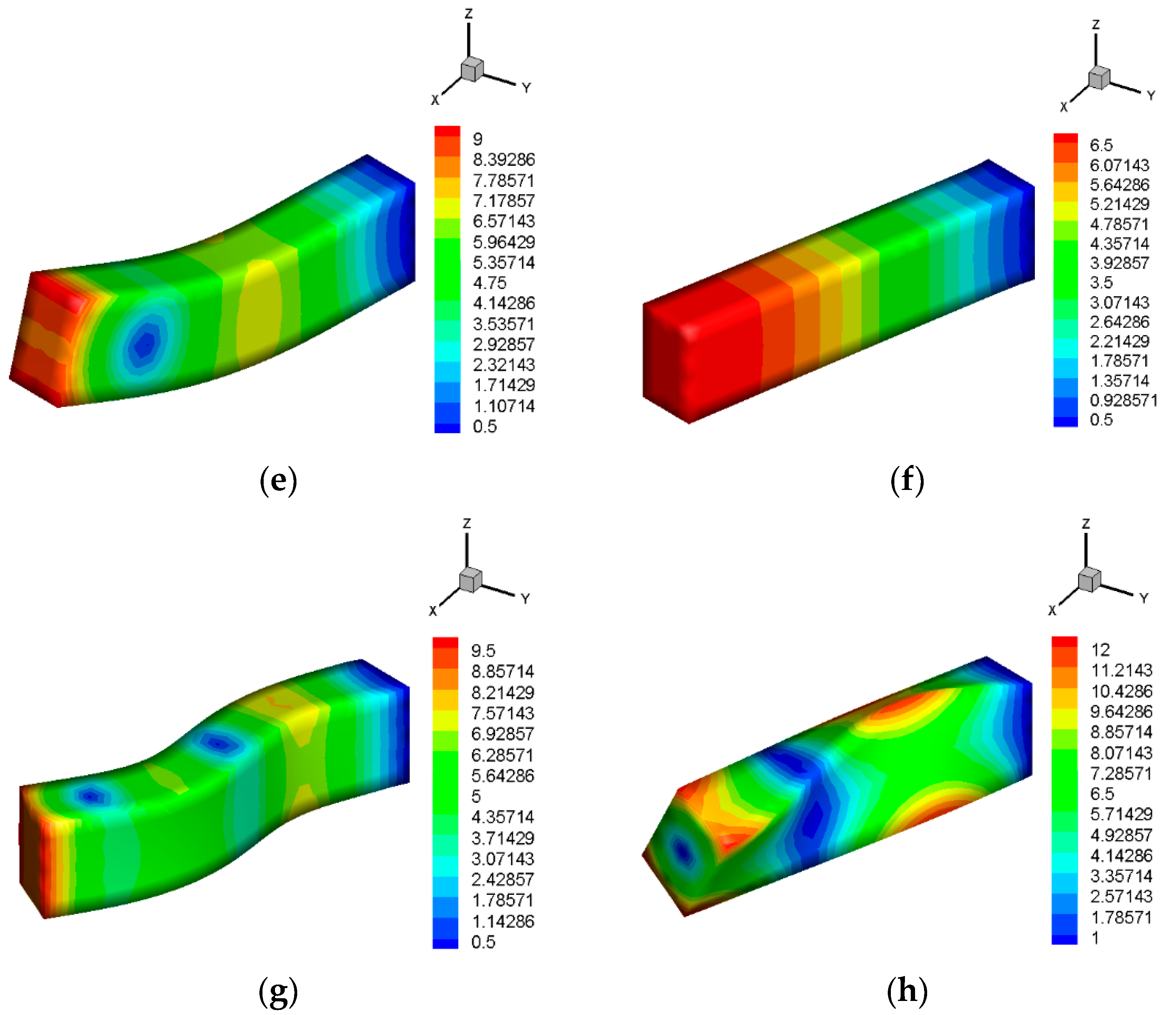
4. Analysis of 3D Examples

This section comprehensively explores the computational accuracy and computational efficiency of E-FEM in 3D models. We used two numerical examples: a cantilever beam structure and an engine connecting rod. The modes of the two numerical examples were calculated using the FEM, ES-FEM, and E-FEM, respectively.

4.1. The Cantilever Beam

Figure 19 shows the structure diagram of the cantilever beam with the geometric parameter of 0.12 m × 0.12 m × 0.72 m. The blue area represents the constrained surface. In the current analysis, we used the following material properties in calculations: elastic modulus E = 70 GPa, Poisson’s ratio v = 0.33, density ρ = 2700 kg/m³. First, we analyzed the calculation accuracy, which was discretized into a grid model with 752 nodes (Figure 19b). For comparison, the model was discretized into an extremely fine mesh (71,771 nodes and 25,200 elements) in ANSYS to obtain the reference solution.

Table 9. Eigenvalues of the first 15 modes of the cantilever beam.

Order	FEM	ES-FEM	E-FEM	Reference
$f_1$	207.73	190.47	189.30	188.67
$f_2$	286.97	276.23	275.90	275.14
$f_3$	1060.39	957.89	936.74	935.04
$f_4$	1155.80	1069.11	1058.69	1055.70
$f_5$	1445.77	1397.85	1393.07	1390.50
$f_6$	1786.54	1782.74	1781.27	1779.90
$f_7$	2823.05	2627.97	2597.55	2591.50
$f_8$	3187.11	2876.26	2811.92	2806.40
$f_9$	3318.56	3207.69	3189.32	3185.40
$f_{10}$	4798.67	4488.68	4420.82	4412.30
$f_{11}$	5323.91	4811.58	4692.26	46,820
$f_{12}$	5343.23	5180.15	5137.22	5133.40
$f_{13}$	5373.71	5307.97	5299.98	5296.20
$f_{14}$	6963.50	6517.56	6397.92	6386.80
$f_{15}$	7500.03	6764.03	6581.80	6564.10

shows the first 15 modal eigenvalues of the cantilever beam, and the relative error is shown in Figure 20, indicating the smallest relative error of E-FEM, hence the highest calculation accuracy among the three methods.

We show the E-FEM calculation of the first 8 modes of a cantilever beam in Figure 21. It is apparent that the proposed E-FEM indeed behaves extremely well in predicting the mode shape.

The cantilever beam was divided into four different sizes of grids to confirm the mesh robustness of E-FEM, with the number of nodes being 153, 399, 752, and 1135. The proposed E-FEM was used to analyze the natural frequency of the grid model, and the findings of FEM and ES-FEM are useful in the comparative analysis [31]. The fifth and 10-order natural frequencies were selected as research objects, and the relative error curve with the number of grid nodes was drawn (Figure 22). Therefore, based on Figure 22: (1) The three numerical methods are convergent; (2) Under a similar number of grid nodes, the calculation error of E-FEM is smaller than that of FEM and ES-FEM. The numerical example shows that E-FEM has good numerical convergence and accuracy.

To investigate a numerical method, we need to analyze its computational efficiency. The same four kinds of grids are used. Figure 23 [32,33] shows the comparison of the calculation efficiency of three different methods (the ratio of the average error of the first 15 modes to time). It can be seen from the figure that the computational efficiency of E-FEM is higher than that of ES-FEM and FEM.

4.2. Engine Connecting Rod

In this section, we performed a modal analysis of an automobile engine connecting rod to confirm the applicability of the proposed method. Figure 24 displays the geometric model of the connecting rod, and the small end of the connecting rod is a fixed constraint. The material parameters include $\mathrm{E}=210$ GPa, $v=0.28$, and $\rho =7900$ kg/m³. The engine connecting rod is discretized into a grid model with 1045 nodes and calculated by three different numerical methods. Notably, the results of 78,526 nodes and 50,491 T-10 elements calculated by ANSYS [34,35] served as reference solutions.

Table 10. First 15 modal eigenvalues of connecting rod.

Order	FEM	ES-FEM	E-FEM	FEM (Fine)	Reference
$f_1$	582.14	528.66	525.51	541.21	522.99
$f_2$	620.30	557.66	552.29	570.38	551.98
$f_3$	1420.51	1105.39	1071.56	1160.39	1053.10
$f_4$	3848.07	3571.62	3539.52	3624.49	3509.70
$f_5$	4650.39	4152.56	4121.00	4256.49	4099.30
$f_6$	5092.29	4688.78	4599.24	4751.62	4527.90
$f_7$	8137.86	7794.29	7744.57	7881.27	7715.50
$f_8$	10,191.39	8462.14	8271.87	8877.15	8104.20
$f_9$	10,948.29	9737.92	9521.96	10,126.97	9242.10
$f_{10}$	11,277.62	9977.75	9800.76	10,134.92	9624.20
$f_{11}$	12,190.94	10,549.44	10,423.65	10,812.64	10,191.00
$f_{12}$	15,146.03	12,015.30	11,664.54	12,570.43	11,327.00
$f_{13}$	17,553.76	15,962.76	15,766.72	16,389.37	15,587.00
$f_{14}$	19,701.50	17,353.71	17,125.72	17,825.40	16,870.00
$f_{15}$	21,737.13	18,887.72	18,588.77	19,513.86	18,040.00

shows the results of the first 15 natural frequencies [36,37]. In addition, FEM was used to calculate the fine mesh model with 5135 nodes; Figure 25 shows the relative errors of the first 15 free mode eigenvalues calculated by E-FEM, ES-FEM, and FEM. Based on the curves and data, the error of the results calculated by E-FEM was significantly smaller than that computed by ES-FEM and FEM, unlike the first 15 modal eigenvalues computed. Therefore, algorithm correctness in dealing with complex models can be preliminarily established. Figure 26 shows the first eight modes.

4.3. Automobile Front Suspension Arm

This section explores the applicability of the proposed method in calculating the complex geometric model of the front suspension arm. The geometric model of the front cantilever is shown in Figure 27, with fixed constraints on the blue surface. The material parameters are $\mathrm{E}=69\mathrm{G}$Pa, $v=0.3$, $\rho =2700$ kg/m³. The results of 54,087 nodes and 34,791 T-10 elements calculated by ANSYS were used as reference solutions.

In addition, FEM was used to calculate the fine mesh model with 5497 nodes, and the outcomes were compared using the three numerical approaches.

Table 11. Eigenvalues of the first 15 modes of the suspension arm.

Order	FEM	ES-FEM	E-FEM	FEM (Fine)	Reference
$f_1$	193.75	159.44	157.18	167.46	155.32
$f_2$	993.98	881.23	862.16	914.48	848.42
$f_3$	1089.25	952.41	945.81	960.43	937.93
$f_4$	1188.08	978.71	962.14	1018.88	950.71
$f_5$	1877.99	1717.52	1703.89	1748.93	1686.60
$f_6$	2134.42	2088.82	2080.74	2091.49	2063.20
$f_7$	2675.84	2217.36	2163.85	2301.22	2130.50
$f_8$	2792.76	2342.92	2291.51	2419.86	2256.90
$f_9$	3279.08	2935.65	2906.53	3001.27	2863.10
$f_{10}$	3790.99	3206.87	3105.93	3306.54	3055.20
$f_{11}$	3857.71	3557.73	3526.29	3610.49	3478.20
$f_{12}$	5209.41	4433.95	4348.32	4554.320	4289.50
$f_{13}$	5422.11	4927.43	4863.51	5013.80	4734.90
$f_{14}$	6159.29	5218.63	4981.44	5324.24	4878.10
$f_{15}$	6637.36	5724.11	5529.93	5848.54	5451.40

shows the results of the natural frequencies of the first 15 orders. In addition, the relative errors of free mode eigenvalues of the first 15 orders calculated by ES-FEM, FEM, and E-FEM are presented in Figure 28. According to the curves and data, the error of the results calculated by E-FEM was remarkably smaller than that computed by ES-FEM and FEM compared to the first 15 modal eigenvalues computed. Therefore, the reliability of the algorithm in dealing with complex models can be established. Figure 29 shows the first eight modes.

5. Conclusions

Based on the traditional FEM, this paper introduced a new basis function and proposed an improved E-FEM. The introduction of new shape functions, geometry matrices, stiffness matrices, and mass matrices improves variable displacement in the triangle and tetrahedral elements of classic FE. The considered numerical experiments can provide the following valuable insights: (1) The technique is used in 2D and 3D free vibration modal analysis, as well as comprehensively compares and analyzes computational efficiency, accuracy, and mesh distortion adaptability. E-FEM-T3 displays high accuracy, good convergence, and significant adaptability to grid distortion with four examples, i.e., the cantilever beam, connecting rod, shear wall, and automobile front suspension arm, under the presumption of not increasing too much calculation. (2) In the forced vibration study, E-FEM-T3, ES-FEM-T3, FEM-Q4, and FEM-T3 harbor extremely consistent vibration periods, whereas E-FEM-T3N6 has a highest amplitude, followed by E-FEM-T3N4, E-FEM-T3N3, ES-FEM-T3, FEM-Q4, and FEM-T3. The E-FEM-T3 has higher calculation precision and better adaptability to grid distortion by comparing computational efficiency to mesh distortion of the above methods in three different 2D models. (3) The proposed E-FEM-T3 element is also less sensitive to mesh distortion than other traditional elements, resulting in reliable numerical results, even when highly distorted models are used. Mesh distortion cannot always be avoided in engineering applications with complicated geometry; therefore, the current method is particularly well suited to these scenarios. (4) Although the current E-FEM-T3 requires no additional nodes compared to the high-order elements, it is more expensive numerically since larger system matrices are formed with more unknown nodal unknowns. Nevertheless, the current E-FEM-T3 still has better calculation precision and efficiency for free and forced vibration analysis solutions. (5) As the number of additional degrees of freedom increases, the convergence rate of the error relative to the calculation time for the three types of E-FEM-T3 solutions decreases; the higher the accuracy, the better the convergence, and the greater the adaptability to the distorted meshes can also be obtained.

References

1. Zienkiewicz, O.C.; Taylor, R.L. The Finite Element Method, 5th ed.; Butterworth-Heinemann: Oxford, UK, 2000. [Google Scholar]
2. To, M. A further study of hybrid strain-based three-node flat triangular shell elements. Finite Elem. Anal. Des. 1998, 31, 135–152. [Google Scholar]
3. Chen, L.; Liu, G.R.; Zeng, K.; Zhang, J. A novel variable power singular element in g space with strain smoothing for bi-material fracture analyses. Eng. Anal. Bound. Elem. 2011, 35, 1303–1317. [Google Scholar] [CrossRef]
4. Liu, G.R.; Dai, K.Y.; Nguyen, T.T. A Smoothed Finite Element Method for Mechanics Problems. Comput. Mech. 2007, 39, 859–877. [Google Scholar] [CrossRef]
5. Liu, G.R.; Nguyen-Thoi, T. Smoothed Finite Element Methods, 1st ed.; CRC Press: Boca Raton, FL, USA, 2010. [Google Scholar]
6. Nguyen-Xuan, H.; Rabczuk, T.; Nguyen-Thoi, T.; Tran, T.; Nguyen-Thanh, N. Computation of limit and shakedown loads using a node-based smoothed finite element method. Int. J. Numer. Methods. Eng. 2012, 90, 287–310. [Google Scholar] [CrossRef]
7. Bordas, S.; Rabczuk, T.; Hung, N.X.; Nguyen, V.P.; Natarajan, S.; Bog, T.; Hiep, N.V. Strain smoothing in FEM and XFEM. Comput. Struct. 2010, 88, 1419–1443. [Google Scholar] [CrossRef]
8. Liu, G.R. A G space theory and a weakened weak (W2) form for a unified formulation of compatible and incompatible methods: Part I Theory. Int. J. Numer. Methods. Engrg. 2010, 81, 1093–1126. [Google Scholar] [CrossRef]
9. Liu, G.R. A G space theory and a weakened weak (W2) form for a unified formulation of compatible and incompatible methods: Part II applications to solid mechanics problems. Int. J. Numer. Methods. Engrg. 2010, 81, 1127–1156. [Google Scholar] [CrossRef]
10. Liu, M.Y.; Gao, G.J.; Zhu, H.F.; Jiang, C.; Liu, G.R. A cell-based smoothed finite element method (CS-FEM) for three-dimensional incompressible laminar flows using mixed wedge-hexahedral element. Eng. Anal. Bound. Elem. 2021, 133, 269–285. [Google Scholar] [CrossRef]
11. Liu, G.R.; Nguyen-Thoi, T.; Nguyen-Xuan, H.; Lam, K.Y. A node-based smoothed finite element method (NS-FEM) for upper bound solutions to solid mechanics problems. Comput. Struct. 2009, 87, 14–26. [Google Scholar] [CrossRef]
12. Duarte, C.A.; Babuška, I.; Oden, J.T. Generalized finite element methods for three dimensional structural mechanics problems. Comput. Struct. 2000, 77, 215–232. [Google Scholar] [CrossRef]
13. Liu, G.R.; Nguyen-Thoi, T.; Lam, K.Y. An edge-based smoothed finite element method (ES-FEM) for static, free and forced vibration analyses of solids. J. Sound Vib. 2009, 320, 1100–1130. [Google Scholar] [CrossRef]
14. Li, W.; Chai, Y.B.; Lei, M.; Li, T.Y. Numerical investigation of the edge-based gradient smoothing technique for exterior Helmholtz equation in two dimensions. Comput. Struct. 2017, 182, 149–164. [Google Scholar] [CrossRef]
15. Chai, Y.B.; You, X.Y.; Li, W.; Huang, Y.; Yue, Z.J.; Wang, M.S. Application of the edge-based gradient smoothing technique to acoustic radiation and acoustic scattering from rigid and elastic structures in two dimensions. Comput. Struct. 2018, 203, 43–58. [Google Scholar] [CrossRef]
16. Zeng, W.; Liu, G.R. Smoothed Finite Element Methods (S-FEM): An Overview and Recent Developments. Arch. Comput. Methods. Eng. 2016, 25, 397–435. [Google Scholar] [CrossRef]
17. Liu, G.R. The smoothed finite element method (S-FEM): A framework for the design of numerical models for desired solutions. Front. Struct. Civ. Eng. 2019, 13, 456–477. [Google Scholar] [CrossRef]
18. Kim, J.; Bathe, K.J. The finite element method enriched by interpolation covers. Comput. Struct. 2013, 116, 35–49. [Google Scholar] [CrossRef]
19. Jeon, H.M.; Lee, P.S.; Bathe, K.J. The MITC3 shell finite element enriched by interpolation covers. Comput. Struct. 2014, 134, 128–142. [Google Scholar] [CrossRef]
20. Jun, H.; Yoon, K.; Lee, P.S.; Bathe, K.J. The MITC3+ shell element enriched in membrane displacements by interpolation covers. Comput. Methods Appl. Mech. Eng. 2018, 337, 458–480. [Google Scholar] [CrossRef]
21. Liu, Y.; Zhang, G.Y.; Lu, H.; Zong, Z. A cell-based smoothed point interpolation method (CS-PIM) for 2D thermoelastic problems. Int. J. Numer. Methods Heat. Fluid. Flow. 2017, 27, 1249–1265. [Google Scholar] [CrossRef]
22. Kim, J.; Bathe, K.J. Towards a procedure to automatically improve finite element solutions by interpolation covers. Comput. Struct. 2014, 131, 81–97. [Google Scholar] [CrossRef]
23. Wu, F.; Zhou, G.; Gu, Q.Y.; Chai, Y.B. An enriched finite element method with interpolation cover functions for acoustic analysis in high frequencies. Eng. Anal. Bound. Elem. 2021, 129, 67–81. [Google Scholar] [CrossRef]
24. Zhou, L.; Wang, J.; Liu, M.; Li, M.; Chai, Y. Evaluation of the transient performance of magneto-electro-elastic based structures with the enriched finite element method. Compos. Struct. 2021, 280, 114888. [Google Scholar] [CrossRef]
25. Li, Y.; Dang, S.; Li, W.; Chai, Y. Free and forced vibration analysis of two-dimensional linear elastic solids using the finite element methods enriched by interpolation cover functions. Mathematics 2022, 10, 456. [Google Scholar] [CrossRef]
26. Khoei, A.R.; Bahmani, B. Application of an enriched FEM technique inthermo-mechanical contact problems. Comput. Mech. 2018, 62, 1127–1154. [Google Scholar] [CrossRef]
27. Khoei, A.R.; Vahab, M.; Hirmand, M. An enriched–FEM technique for numerical simulation of interacting discontinuities in naturally fractured porous media. Comput. Methods Appl. Mech. Eng. 2017, 17, 169–232. [Google Scholar] [CrossRef]
28. Wu, C.T.; Koishi, M. Three-dimensional meshfree-enriched finite element formulation for micromechanical hyper elastic modeling of particulate rubber composites. Int. J. Numer. Methods Eng. 2012, 91, 1137–1157. [Google Scholar] [CrossRef]
29. Yang, Y.T.; Xu, D.D.; Zheng, H. Application of the three-node triangular element with continuous nodal stress for free vibration analysis. Comput. Struct. 2016, 169, 69–80. [Google Scholar] [CrossRef]
30. Dai, K.Y.; Liu, G.R. Free and forced vibration analysis using the smoothed finite element method (SFEM). J. Sound Vib. 2007, 301, 803–820. [Google Scholar] [CrossRef]
31. Chen, J.S.; Wu, C.T.; Yoon, S.; You, Y. A stabilized confirming nodal integration for Galerkin meshfree methods. Int. J. Numer. Methods Eng. 2001, 53, 2587–2615. [Google Scholar] [CrossRef]
32. Ham, S.; Bathe, K.J. A finite element method enriched for wave propagation problems. Comput. Struct. 2012, 94, 1–12. [Google Scholar] [CrossRef]
33. Chai, Y.B.; Bathe, K.J. Transient wave propagation in inhomogeneous media with enriched overlapping triangular elements. Comput. Struct. 2020, 237, 106273. [Google Scholar] [CrossRef]
34. Li, Y.; Liu, G.R.; Yue, J.H. A novel node-based smoothed radial point interpolation method for 2D and 3D solid mechanics problems. Comput. Struct. 2018, 196, 157–172. [Google Scholar] [CrossRef]
35. Liu, G.R.; Gu, Y.T. An Introduction to Meshfree Methods and Their Programming; Springer: Berlin/Heidelberg, Germany, 2005. [Google Scholar]
36. Gui, Q.; Zhou, Y.; Li, W.; Chai, Y.B. Analysis of two-dimensional acoustic radiation problems using the finite element with cover functions. Appl. Acoust. 2022, 185, 108408. [Google Scholar] [CrossRef]
37. Chai, Y.B.; Li, W.; Liu, Z.Y. Analysis of transient wave propagation dynamics using the enriched finite element method with interpolation cover functions. Appl. Math. Comput. 2022, 412, 126564. [Google Scholar] [CrossRef]
38. Liu, G.R.; Gu, Y.T. A local radial point interpolation method (LRPIM) for free vibration analyses of 2-D solids. J. Sound Vib. 2001, 246, 29–46. [Google Scholar] [CrossRef]
39. Gu, Y.; Lei, J. Fracture mechanics analysis of two-dimensional cracked thin structures (from micro- to nano-scales) by an efficient boundary element analysis. Results Math. 2021, 11, 100172. [Google Scholar] [CrossRef]
Figure 1. The enriched cover interpolation sub-domains that employ a standard triangular mesh (a,b) and tetrahedral mesh (c,d) for E-FEM: (a) The cover region ( ε i ) for enriched interpolation covers and the typical linear interpolation functions (b) Local coordinates and physical coordinates of triangular element nodes; (c) Displacement of tetrahedral element node after introducing basis function; (d) The natural coordinate system of the tetrahedral element.
Machines 11 00587 g001
Figure 2. 2D cantilever beam.
Machines 11 00587 g002
Figure 3. Triangle mesh for cantilever beam in Figure 4: (a) Mesh a (10 × 1); (b) Mesh b (20 × 2); (c) Mesh c (40 × 4).
Machines 11 00587 g003aMachines 11 00587 g003b
Figure 4. Comparison of calculation frequency accuracy of two modes: (a) Mode two; (b) Mode four; (c) Mode two; (d) Mode four.
Machines 11 00587 g004
Figure 5. Convergence of the calculated frequency error of two modes: (a) Mode two; (b) Mode four.
Machines 11 00587 g005
Figure 6. The top ten vibration modes of the cantilever beam calculated by E-FEM: (a) Mode one; (b) Mode two; (c) Mode three; (d) Mode four; (e) Mode five; (f) Mode six; (g) Mode seven; (h) Mode eight; (i) Mode nine; (j) Mode ten.
Machines 11 00587 g006aMachines 11 00587 g006b
Figure 7. Distorted element mesh.
Machines 11 00587 g007
Figure 8. Calculated frequency error of the first mode for the distortion sensitivity test.
Machines 11 00587 g008
Figure 9. The distorted grids of Figure 4 (mesh: 20 × 2 ):(a) Mesh A; (b) Mesh B; (c) Mesh C.
Machines 11 00587 g009
Figure 10. Grid distortion adaptability comparison.
Machines 11 00587 g010
Figure 11. The comparison of computational efficiency for two modes: (a) Mode two; (b) Mode four.
Machines 11 00587 g011
Figure 12. Comparison of transient responses of a cantilever beam by E-FEM-T3: (a) Results of all 6 algorithms; (b) Analysis of the performance of 4 algorithms; (c) Multi-basis function curve of forced vibration; (d) Partial enlarged view of Figure 12b; (e) Partial enlarged view of Figure 12c.
Machines 11 00587 g012aMachines 11 00587 g012bMachines 11 00587 g012c
Figure 13. A shear wall.
Machines 11 00587 g013
Figure 14. The grid of a shear wall grid.
Machines 11 00587 g014
Figure 15. First 10 vibration modes of the shared wall computed using E-FEM: (a) Mode one; (b) Mode two; (c) Mode three; (d) Mode four; (e) Mode five; (f) Mode six; (g) Mode seven; (h) Mode eight; (i) Mode nine; (j) Mode ten.
Machines 11 00587 g015aMachines 11 00587 g015b
Figure 16. A geometric model and boundary conditions of an automobile connecting rod.
Machines 11 00587 g016
Figure 17. Mesh A of the connecting rod.
Machines 11 00587 g017
Figure 18. First 10 vibration modes of the connecting rod computed by E-FEM: (a) Mode one; (b) Mode two; (c) Mode three; (d) Mode four; (e) Mode five; (f) Mode six; (g) Mode seven; (h) Mode eight; (i) Mode nine; (j) Mode ten.
Machines 11 00587 g018aMachines 11 00587 g018b
Figure 19. A cantilever model: (a) geometric model (b) mesh.
Machines 11 00587 g019
Figure 20. Relative error of first 15 modal eigenvalues of the cantilever beam.
Machines 11 00587 g020
Figure 21. Calculation of the first 8 modes of a cantilever beam using E-FEM: (a) Mode one; (b) Mode two; (c) Mode three; (d) Mode four; (e) Mode five; (f) Mode six; (g) Mode seven; (h) Mode eight.
Machines 11 00587 g021aMachines 11 00587 g021b
Figure 22. Convergence comparison: (a) Mode five; (b) Mode ten.
Machines 11 00587 g022
Figure 23. Comparison of computational efficiency: (a) Mode five; (b) Mode ten.
Machines 11 00587 g023
Figure 24. Connecting rod model: (a) geometric model; (b) mesh.
Machines 11 00587 g024
Figure 25. Relative error of first 15 modal eigenvalues of connecting rod.
Machines 11 00587 g025
Figure 26. First 8 modal shapes of connecting rod calculated by E-FEM: (a) Mode one; (b) Mode two; (c) Mode three; (d) Mode four; (e) Mode five; (f) Mode six; (g) Mode seven; (h) Mode eight.
Machines 11 00587 g026
Figure 27. Vehicle suspension arm model: (a) geometric model (b) mesh.
Machines 11 00587 g027
Figure 28. Relative error of first 15 modal eigenvalues of the suspension arm.
Machines 11 00587 g028
Figure 29. First 8 modes of automobile suspension arm calculated by E-FEM: (a) Mode one;(b) Mode two; (c) Mode three; (d) Mode four; (e) Mode five; (f) Mode six; (g) Mode seven; (h) Mode eight.
Machines 11 00587 g029aMachines 11 00587 g029b