Study on Sinusoidal Post-Buckling Deformation of Coiled Tubing in Horizontal Wells Based on the Separation Constant Method

Abstract

In this paper, a set of partial differential equations considering the dynamic effects of the coiled tubing (CT) is established based on the bending theory of slender beams considering the axial loads. The analytical solution of sinusoidal deformation with the time term is obtained. The critical load of coiled tubing during sinusoidal buckling and the change of half-wave number during sinusoidal post-buckling are studied through the introduction of the necessary conditions, solution and the separation constant. The contact force of coiled tubing with sinusoidal post-buckling on the horizontal well wall is analyzed. The results show that the critical load for sinusoidal buckling of fixed-size CT is related to the section angular acceleration coefficient. The half-wave number produced by the sinusoidal post-buckling bending of the CT gradually decreases during compression. The contact force of the deformed CT to the borehole wall is related to the compression speed of the CT. By introducing the dynamic term and the separation constant, this research model can provide a theoretical basis for studying the transformation of the CT from sinusoidal buckling to helical buckling.

1. Introduction

With the advantages of fast and efficient operation, little damage to the formation, and low cost of use, CT is widely used in oil and gas field workover, drilling, completion, logging, and other operations, and plays a very important role in oil and gas field exploration and development. The working environment during downhole operations is very complex, and CT often undergoes sinusoidal and helical buckling, which affects the working efficiency. The CT moves in the well with friction and even locks up in extreme cases [1,2,3]. Since Rubinski conducted a study on the buckling behavior of tubular string [4], Mitchell has extended the buckling model of Rubinski and solved the helical buckling model problem using numerical methods [5]. P.R. Paslay and D.B. Bogy use the energy method to analyze the stability of a tubular string in an oblique straight section and derive a formula for calculating the critical load when sinusoidal buckling of the tubular occurs [6]. Dawson and Paslay have given a formula for calculating the critical load of tubular string instability in high-angle wells [7], considering buoyancy weight per length of the pipe and ignoring friction. Subsequently, many scholars have begun to study the buckling deformation of tubular columns [8,9,10,11]. Chen et al. study the buckling behavior of tubular string in the horizontal well using the energy method [12]. Rasoul et al. study the effects of shear deformation and rotary inertia on post-buckling behavior [13] and Xing and Gao analyze the buckling of pipe string under the action of friction force, the coupling effect between axial force and friction force is solved for the first time [14]. Gao and Huang study the buckling behavior by using the energy method and the tubular string buckling equation [15].

As the research progresses, the researchers have found that there is a considerable deviation between the theoretical buckling deformation of the tube column and the actual occurrence of buckling deformation [16,17]. Researchers with different initial conditions are able to obtain different calculation results for the tubular string buckling. Robert and Mitchell add axial torque to model the tubular subjected to axial force and torque [18]; He et al. give an algorithm for buckling loads in three dimensions [19]. Zhu et al. investigate the effect of initial curvature on the buckling deformation of the tubular column [20]. Gao and Miska introduce the effect of frictional forces on the deformation of the tubular column [21,22]. However, the shape of the tubular string undergoes a complex transformation with compression during the transition from straight form to sinusoidal buckling or from sinusoidal buckling to helical buckling, such as the curve of the wellbore or the continuous contact between the tubular string and the wellbore and so on [23]. However, there is no unified model to represent the transition from sinusoidal buckling to helical buckling of the tubular string so far [24].

In order to study the conversion process from sinusoidal buckling to helical buckling in depth, this paper adopts a new analytical method to study the sinusoidal post-buckling deformation of a tubular string with a straight initial configuration in a horizontal well subjected to axial load compression by using dynamic factors and introducing the separation constant. Firstly, a mathematical model of the bending deformation of the horizontal coiled tubing containing the dynamic term is established. By introducing the separation constant, the sine analytical solution and the sine critical load formula including the section angular acceleration coefficient are obtained. Secondly, the range of the separation constant after sinusoidal buckling deformation is obtained by the energy method, and the calculation formulas of compression displacement and axial load including the separation constant and time term are derived. Finally, the force changes of the CT with sinusoidal post-buckling on the well wall under different velocities and different axial loads are analyzed.

2. Theoretical Model

2.1. Coiled Tubing Buckling Equation

CT’s deformation under axial load occurs in three shapes: sinusoidal buckling configuration, sinusoidal–helical buckling hybrid configuration, and helical buckling conformation. Due to the complexity of the model and the excessive actual boundary conditions, the following assumptions are made under the premise of ensuring that the results are not distorted.

(1)

The length along its axis remains invariable when the CT is deformed.

(2)

The influence of fluids, such as downhole mud, on the mechanics of CT is neglected.

(3)

The wellbore and CT are circular in cross-section.

(4)

There is deformation of CT in the horizontal well sections at continuous contact.

(5)

The clearance between the CT and the wellbore is much smaller than the CT length.

(6)

The effects of the CT rotation and torsion are neglected.

(7)

The initial shape of the CT before deformation occurs is straight.

(8)

The CT is connected with two pin ends.

As shown in Figure 1, point O₁ is established at the center of the circle of the horizontal shaft, the x-axis is the vertical direction, the y-axis is the horizontal direction, and the z-axis is the direction of the horizontal well axis to establish the coordinate system. The radius of the wellbore is r_s and the radius of the outer circle of the tubular string is r_p. The radial clearance between the wellbore and the CT is $r_c=r_s-r_p$. The unit vectors of the X-axis, Y-axis and Z-axis correspond to i, j, and k. e_t, e_n, and e_b are the unit vectors in the tangential direction, the main normal, and the minor normal at a point of the deformed coiled tubing, respectively. r_c indicates the vector diameter from origin O to contact point C, r_o is the radius vector from the original point O to the center of the wellbore O₁, and r is the radius vector from the origin O to the center of the micro segment O₂.

The dynamic equilibrium equations for a unit length of the tubular string is

$$\frac{\partial V}{\partial s}+F=\frac{m}{\Delta s}\frac{{\partial }^{2}r}{\partial t^2}$$

(1)

where F is the vector of external forces per unit length of the CT, the gravity per unit length of the coiled tubing is q, V is the vector of internal forces on the micro segment of the CT, Δs is the arc length of the micro segment of the CT, m is the mass of the micro segment of the CT, and t is the motion time of micro segment.

The equations of momentum theorem and moment of momentum theorem of a unit length of the tubular string after neglecting small quantities are

$$\frac{\partial \left(mv\right)}{\partial t}=\left(V+\Delta V\right)-V+F\Delta s$$

(2)

$$\frac{\partial H}{\partial t}=M+\frac{\partial \psi }{\partial s}+e_t\times V$$

(3)

According to the definition of angular momentum, we can obtain

$$H=\rho A\left(r-r_o\right)\times \left[\Omega \times \left(r-r_o\right)+v_{z}k\right]+I_c\omega$$

(4)

where M is the external torque of the external force on the CT per unit length to the center O₂ of the CT, Ψ is the internal moment on the micro segment of the CT, H is the moment of momentum per unit length of the CT to the center of the wellbore, I_c is the rotational inertia of a unit length of CT around its axis. ω is the angular velocity vector of the rotation of the CT on its axis, ρ is the density of the CT, A is the cross-sectional area of the CT, and Ω is the angular velocity vector of the rotation of the center point of a unit length of CT in the XY-plane around the borehole center. The subscripts X, Y, and Z represent the components of each vector parameter in the X-axis, Y-axis, and Z-axis, respectively.

The motion of the CT In contact with the horizontal well when deformation occurs can be split into two directions: the direction of motion along the Z-axis and the rotation along the XY-plane. Assume that the friction coefficients for each of the two motions are μ_z and μ_xy. The following conditions are satisfied.

$$\left\{\begin{array}{l}x=r_c\cos \theta \\ y=r_c\sin \theta \end{array}\right.$$

The expressions for the friction f and the external force vector F per unit length of the CT in contact with the horizontal well are

$$f=sign\left(\theta \right)\left({\mu }_{xy}N\sin \theta \cdot i-{\mu }_{xy}N\cos \theta \cdot j\right)-{\mu }_{z}Nk$$

(5)

$$\begin{array}{l}F=\left[-N\cos \theta +sign\left(\theta \right){\mu }_{xy}N\sin \theta +\rho Ag\right]i\\ +\left[-N\sin \theta -sign\left(\theta \right){\mu }_{xy}N\cos \theta \right]j-{\mu }_{z}Nk\end{array}$$

(6)

where $\mathrm{sign}\left(\theta \right)=1$ when the CT micro section rotates clockwise, and $\mathrm{sign}\left(\theta \right)=-1$ when the CT micro section rotates counterclockwise. θ is the angular displacement of the section when the CT undergoes buckling deformation and N is the contact force of the well wall on the unit length of the CT.

Substituting Equation (6) into Equation (1) and expanding it gives

$$\left\{\begin{array}{l}\frac{\partial V_x}{\partial s}=\rho A\frac{{\partial }^{2}x}{\partial t^2}+\left(N\cos \theta -sign\left(\theta \right){\mu }_{xy}N\sin \theta -\rho Ag\right)\\ \frac{\partial V_y}{\partial s}=\rho A\frac{{\partial }^{2}y}{\partial t^2}+\left(N\sin \theta +sign\left(\theta \right){\mu }_{xy}N\cos \theta \right)\\ \frac{\partial V_z}{\partial s}=\rho A\frac{{\partial }^{2}z}{\partial t^2}+{\mu }_{z}N\end{array}\right.$$

(7)

When the micro segment of the CT moves to satisfy

$$\frac{\partial x}{\partial t}=-\frac{\partial \theta }{\partial t}{r}_c\sin \theta$$

(8)

$$\frac{\partial y}{\partial t}=\frac{\partial \theta }{\partial t}{r}_c\cos \theta$$

(9)

Substituting the above equation into Equation (3) and from the stress as a function of strain [25,26], we can obtain the expanded form of the momentum moment theorem about the micro section of the CT.

$$\begin{array}{c}\rho A\left(\mathbf{r}-{\mathbf{r}}_o\right)\times \left[\frac{\partial \mathbf{\Omega }}{\partial t}\times \left(\mathbf{r}-{\mathbf{r}}_o\right)+\mathbf{\Omega }\times \left(\mathbf{v}-{\mathbf{v}}_o\right)+\frac{{\partial }^{2}z}{\partial t^2}\mathbf{k}\right]-\rho A\left({\mathbf{v}}_o\times \mathbf{v}\right)\hfill \\ =\mathbf{M}+\frac{\partial \left\{EI\left[\left(\frac{\partial y}{\partial s}\frac{{\partial }^{2}z}{\partial s^2}-\frac{\partial z}{\partial s}\frac{{\partial }^{2}y}{\partial s^2}\right)\mathbf{i}+\left(\frac{\partial z}{\partial s}\frac{{\partial }^{2}x}{\partial s^2}-\frac{\partial x}{\partial s}\frac{{\partial }^{2}z}{\partial s^2}\right)\mathbf{j}+\left(\frac{\partial x}{\partial s}\frac{{\partial }^{2}y}{\partial s^2}-\frac{\partial y}{\partial s}\frac{{\partial }^{2}x}{\partial s^2}\right)\mathbf{k}\right]\right\}}{\partial s}\hfill \\ +\left(\frac{\partial y}{\partial s}{V}_z-\frac{\partial z}{\partial s}{V}_y\right)\mathbf{i}+\left(\frac{\partial z}{\partial s}{V}_x-\frac{\partial x}{\partial s}{V}_z\right)\mathbf{j}+\left(\frac{\partial x}{\partial s}{V}_y-\frac{\partial y}{\partial s}{V}_x\right)\mathbf{k}\hfill \end{array}$$

(10)

where E is the elastic modulus and I is the moment of inertia. Since the coordinate center O of the coordinate system coincides with the wellbore center O₁, so $r_o=z_{o}k$ and $x_o=y_o=0$. $v_o$ is the velocity vector of point O₁, and the velocity direction moves along the Z-axis. v_ox, v_oy, and v_oz, respectively, represent the components of the velocity $v_o$ in the X-axis, Y-axis, and Z-axis, which must be v_ox = v_oy = 0. Equation (11) becomes

$$\left\{\begin{array}{l}EI\left(\frac{\partial y}{\partial s}\frac{{\partial }^{3}z}{\partial s^3}-\frac{\partial z}{\partial s}\frac{{\partial }^{3}y}{\partial s^3}\right)+\left(\frac{\partial y}{\partial s}{V}_z-\frac{\partial z}{\partial s}{V}_y\right)={\xi }_1\\ EI\left(\frac{\partial z}{\partial s}\frac{{\partial }^{3}x}{\partial s^3}-\frac{\partial x}{\partial s}\frac{{\partial }^{3}z}{\partial s^3}\right)+\left(\frac{\partial z}{\partial s}{V}_x-\frac{\partial x}{\partial s}{V}_z\right)={\xi }_2\\ EI\left(\frac{\partial x}{\partial s}\frac{{\partial }^{3}y}{\partial s^3}-\frac{\partial y}{\partial s}\frac{{\partial }^{3}x}{\partial s^3}\right)+\left(\frac{\partial x}{\partial s}{V}_y-\frac{\partial y}{\partial s}{V}_x\right)={\xi }_3\end{array}\right.$$

(11)

where:

$$\begin{array}{c}{\xi }_1=\rho A\left(y\frac{{\partial }^{2}z}{\partial t^2}+\frac{\partial z}{\partial t}\frac{\partial y}{\partial t}\right)-M_x,\\ {\xi }_2=\rho A\left(-x\frac{{\partial }^{2}z}{\partial t^2}-\frac{\partial z}{\partial t}\frac{\partial x}{\partial t}\right)-M_y,\\ {\xi }_3=\rho A\left[x\left(\frac{{\partial }^2\theta }{\partial t^2}y+\frac{\partial \theta }{\partial t}\frac{\partial y}{\partial t}\right)-y\left(\frac{{\partial }^2\theta }{\partial t^2}x+\frac{\partial \theta }{\partial t}\frac{\partial x}{\partial t}\right)\right]-M_z.\end{array}$$

Taking the derivative of arc length s at both ends of Equation (11), substituting Equations (1), (7)–(9) and (11) into the equation, respectively, and ignoring the small quantities, we can obtain partial differential Equations (12) and (13) for the dynamic balance of horizontal coiled tubing when bending and deforming under axial load.

$$\begin{array}{l}EI{r}_c\left[\frac{{\partial }^{3}z}{\partial s^3}\frac{{\partial }^2\theta }{\partial s^2}+\frac{\partial \theta }{\partial s}\frac{{\partial }^{4}z}{\partial s^4}+\frac{{\partial }^{2}z}{\partial s^2}{\left(\frac{\partial \theta }{\partial s}\right)}^3-\frac{{\partial }^{2}z}{\partial s^2}\frac{{\partial }^3\theta }{\partial s^3}+6\frac{\partial z}{\partial s}{\left(\frac{\partial \theta }{\partial s}\right)}^2\frac{{\partial }^2\theta }{\partial s^2}-\frac{\partial z}{\partial s}\frac{{\partial }^4\theta }{\partial s^4}\right]\\ +r_c\frac{\partial }{\partial s}\left(V_z\frac{\partial \theta }{\partial s}\right)-\frac{\partial }{\partial s}\left(\frac{\partial z}{\partial s}{V}_y\right)\cos \theta +\frac{\partial }{\partial s}\left(\frac{\partial z}{\partial s}{V}_x\right)\sin \theta =\frac{\partial {\xi }_1}{\partial s}\cos \theta +\frac{\partial {\xi }_2}{\partial s}\sin \theta \end{array}$$

(12)

$$\begin{array}{l}EI{r}_c\left[4\frac{\partial z}{\partial s}\frac{\partial \theta }{\partial s}\frac{{\partial }^3\theta }{\partial s^3}-\frac{{\partial }^{3}z}{\partial s^3}{\left(\frac{\partial \theta }{\partial s}\right)}^2+3\frac{{\partial }^{2}z}{\partial s^2}\frac{\partial \theta }{\partial s}\frac{{\partial }^2\theta }{\partial s^2}-\frac{\partial z}{\partial s}{\left(\frac{\partial \theta }{\partial s}\right)}^4+3\frac{\partial z}{\partial s}{\left(\frac{{\partial }^2\theta }{\partial s^2}\right)}^2\right]\\ -r_c{V}_z{\left(\frac{\partial \theta }{\partial s}\right)}^2-\frac{\partial }{\partial s}\left(\frac{\partial z}{\partial s}{V}_y\right)\sin \theta -\frac{\partial }{\partial s}\left(\frac{\partial z}{\partial s}{V}_x\right)\cos \theta =\frac{\partial {\xi }_1}{\partial s}\sin \theta -\frac{\partial {\xi }_2}{\partial s}\cos \theta \end{array}$$

(13)

In this paper, it is assumed that the CT is incompressible along the axial direction, the length of the CT is larger than the diameter of the wellbore, and the angle θ changes very little with the axial coordinate value, which can be considered as $ds\approx dz$. Assuming that the axial load on each micro section of the CT is the same, the axial load satisfies $F_z=V_z$. According to Equations (12) and (13), the partial differential equations considering the dynamic effect when the CT in the horizontal wellbore is compressed and bent by axial load can be obtained, as shown in Equation (14).

$$\left\{\begin{array}{c}{EIr}_c\left[6{\left(\frac{\partial \theta }{\partial z}\right)}^2\frac{{\partial }^2\theta }{\partial z^2}-\frac{{\partial }^4\theta }{\partial z^4}\right]+r_c\frac{\partial }{\partial z}\left(F_z\frac{\partial \theta }{\partial z}\right)-sign\left(\theta \right){\mu }_{xy}N+{\mu }_z{r}_{p}N\frac{\partial \theta }{\partial z}-\rho Agsin\theta \hfill \\ =\rho A{r}_c\left[\frac{{\partial }^{2}z}{\partial t^2}\frac{\partial \theta }{\partial z}+\frac{\partial }{\partial z}\left(\frac{\partial z}{\partial t}\frac{\partial \theta }{\partial t}\right)+\frac{{\partial }^2\theta }{\partial t^2}\right]\hfill \\ {EIr}_c\left[4\frac{\partial \theta }{\partial z}\frac{{\partial }^3\theta }{\partial z^3}-{\left(\frac{\partial \theta }{\partial z}\right)}^4+3{\left(\frac{{\partial }^2\theta }{\partial z^2}\right)}^2\right]-r_c{F}_z{\left(\frac{\partial \theta }{\partial z}\right)}^2-N+{\mu }_z{r}_p\frac{\partial N}{\partial z}+\rho Agcos\theta \hfill \\ =\rho A{r}_c\left[\frac{\partial }{\partial z}\left(\frac{{\partial }^{2}z}{\partial t^2}\right)-\frac{\partial \theta }{\partial t}\left(\frac{\partial z}{\partial t}\frac{\partial \theta }{\partial z}+\frac{\partial \theta }{\partial t}\right)\right]\hfill \end{array}\right.$$

(14)

Mitchell [27] analyzes the bending deformation of the CT in the wellbore assuming that the CT in static condition. In contrast, the system of Equation (14) considers the effect of deformation on the CT due to motion during the deformation process. If friction and dynamic effects are ignored, the equation can be simplified to the form of $\beta =0$ in Mitchell’s conclusion as follows:

$$\left\{\begin{array}{l}EI\left[6{\left(\frac{\partial \theta }{\partial z}\right)}^2\frac{{\partial }^2\theta }{\partial z^2}-\frac{{\partial }^4\theta }{\partial z^4}\right]+\frac{\partial }{\partial z}\left(F_z\frac{\partial \theta }{\partial z}\right)-\frac{\rho Ag}{r_c}\sin \theta =0\\ EI\left[4\frac{\partial \theta }{\partial z}\frac{{\partial }^3\theta }{\partial z^3}-{\left(\frac{\partial \theta }{\partial z}\right)}^4+3{\left(\frac{{\partial }^2\theta }{\partial z^2}\right)}^2\right]-F_z{\left(\frac{\partial \theta }{\partial z}\right)}^2-\frac{N}{r_c}+\frac{\rho Ag}{r_c}\cos \theta =0\end{array}\right.$$

The CT is in continuous contact with the well wall, the contact force N varies little with the axial coordinate Z, the radius r_p of the continuous tubular string is also small compared to the length of the tubular, and the friction coefficient ${\mu }_z$ is less than 1, so the value of ${\mu }_z{r}_{p}N\partial \theta /\partial z$ is very small, and the value of ${\mu }_z{r}_p\partial N/\partial z$ is also very small in the system of Equation (14). It shows that the influence of axial friction force on the deformation of the CT is much smaller than that of radial friction force at the beginning of the deformation. These are the same conclusions as those obtained by Gao [22] and Miska [18].

2.2. Equation Dimensionless

Equation (14) does the following parameter transformations:

$$\chi =2{\left(\frac{EIq}{r_c}\right)}^{\frac{1}{2}}$$

that is, $\overline{z}=z/\varsigma$, ${\overline{F}}_z=F_z/\chi$, $\overline{t}=t/\delta$, and $\overline{N}=N/q$.

Equation (15) is a non-dimensional partial differential equation set for horizontal coiled tubing deformation considering dynamic effects.

$$\left\{\begin{array}{c}6{\left(\frac{\partial \theta }{\partial \overline{z}}\right)}^2\frac{{\partial }^2\theta }{\partial {\overline{z}}^2}-\frac{{\partial }^4\theta }{\partial {\overline{z}}^4}+2{\overline{F}}_z\frac{{\partial }^2\theta }{\partial {\overline{z}}^2}-sign\left(\theta \right){\mu }_{xy}\overline{N}+{\mu }_z\overline{N}\frac{r_s}{\varsigma }\frac{\partial \theta }{\partial \overline{z}}-sin\theta \hfill \\ =\frac{r_c^4}{I}\left(\frac{{\partial }^2\overline{z}}{\partial {\overline{t}}^2}\frac{\partial \theta }{\partial \overline{z}}+2\frac{{\partial }^2\theta }{\partial {\overline{t}}^2}\right)\hfill \\ 4\frac{\partial \theta }{\partial \overline{z}}\frac{{\partial }^3\theta }{\partial {\overline{z}}^3}-{\left(\frac{\partial \theta }{\partial \overline{z}}\right)}^4+3{\left(\frac{{\partial }^2\theta }{\partial {\overline{z}}^2}\right)}^2-2{\overline{F}}_z{\left(\frac{\partial \theta }{\partial \overline{z}}\right)}^2-\overline{N}+{\mu }_z\frac{r_p}{\varsigma }\frac{\partial \overline{N}}{\partial \overline{z}}+cos\theta \hfill \\ =\frac{r_c^4}{I}\left[\frac{\frac{{\partial }^3\overline{z}}{\partial {\overline{t}}^3}}{\frac{\partial \overline{z}}{\partial \overline{t}}}-2{\left(\frac{\partial \theta }{\partial \overline{t}}\right)}^2\right]\hfill \end{array}\right.$$

(15)

The equation is a fourth-order nonlinear partial differential equation, and it is difficult to obtain an analytical solution. It is assumed that the initial deformation of the CT is small, and $d\theta /d\overline{z}$ is a small quantity. ${\partial }^2\overline{z}/\partial {\overline{t}}^2$ is the axial acceleration of the micro section. If this term is included, the equation is a nonlinear partial differential equation. Non-linear factors are not considered in this study, so this factor is ignored in a reasonable way. Assuming that the lowering speed of the CT does not change much, it becomes a linear partial differential equation that is easy to solve after being omitted. The initial deformation of the CT is small, and the influence of friction and high-order small quantities are ignored [21]. Equation (16) is the simplified dimensionless equation considering dynamic effects. After simplification, Equation (15) becomes the following linear differential equation.

$$\left\{\begin{array}{l}\frac{{\partial }^4\theta }{\partial {\overline{z}}^4}-2{\overline{F}}_z\frac{{\partial }^2\theta }{\partial {\overline{z}}^2}+\theta =-2\frac{r_c{}^4}{I}\frac{{\partial }^2\theta }{\partial {\overline{t}}^2}\\ 4\frac{\partial \theta }{\partial \overline{z}}\frac{{\partial }^3\theta }{\partial {\overline{z}}^3}+3{\left(\frac{{\partial }^2\theta }{\partial {\overline{z}}^2}\right)}^2-2{\overline{F}}_z{\left(\frac{\partial \theta }{\partial \overline{z}}\right)}^2-\overline{N}+1-\frac{{\theta }^2}{2}+\frac{{\theta }^4}{24}=-2\frac{r_c{}^4}{I}{\left(\frac{\partial \theta }{\partial \overline{t}}\right)}^2\end{array}\right.$$

(16)

3. Results and Discussion

3.1. Conditional Analysis of Solutions

A solution to the system of Equation (16) is assumed to be

$$\theta \left(\overline{z},\overline{t}\right)=\mathrm{\Phi }\left(\overline{z}\right)G\left(\overline{t}\right)$$

where Ф$\left(\overline{z}\right)$ is a function of $\overline{z}$ only and G$\left(\overline{t}\right)$ is a function of $\overline{t}$ only. Equation (16) can be rewritten as

$$\left\{\begin{array}{l}\frac{1}{\mathrm{\Phi }}\frac{{\partial }^4\mathrm{\Phi }}{\partial {\overline{z}}^4}-2{\overline{F}}_z\frac{1}{\mathrm{\Phi }}\frac{{\partial }^2\mathrm{\Phi }}{\partial {\overline{z}}^2}+1=\lambda \\ -2\frac{r_c{}^4}{I}\frac{1}{\mathrm{G}}\cdot \frac{{\partial }^{2}G}{\partial {\overline{t}}^2}=\lambda \end{array}\right.$$

(17)

where λ is the separation constant.

It can be seen that the boundary conditions are different, and the solutions of Equation (17) are different. In this paper, only the tubular string with two ends hinged in the initial shape of the straight line is studied, and the boundary conditions are as follows:

$${\left.\frac{{\partial }^2\theta }{\partial {\overline{z}}^2}\right|}_{\overline{z}=0}={\left.\frac{{\partial }^2\theta }{\partial {\overline{z}}^2}\right|}_{\overline{z}=\overline{L}}=0, \theta \left(0,\overline{t}\right)=\theta \left(\overline{L},\overline{t}\right)=0, \theta \left(\overline{z},0\right)=0$$

One solution of equation system Equation (16) is

$$\theta \left(\overline{z},\overline{t}\right)=M\left(e^{\sqrt{-\frac{\lambda }{Q}}\overline{t}}-e^{-\sqrt{-\frac{\lambda }{Q}}\overline{t}}\right)\sin \left(\frac{\pi n}{\overline{L}}\overline{z}\right)$$

(18)

where M is any constant. Obviously, the value of M is different for different boundary conditions. Equation (18) can be expressed in the following form.

$$\theta =A_n\sin \left(\frac{n\pi \overline{z}}{\overline{L}}\right)$$

(19)

where $\overline{L}$ represents the axial dimensionless length of the CT after compression and n is the half-wave number. By solving the partial differential equation, we know that due to the existence of the separation constant, there are many solutions to the equation. In Equation (19), the expression of the amplitude A_n is different according to the value range of the separation constant. The necessary condition for this formula to be established is

$${\overline{F}}_z=-\frac{1}{2}\left[\frac{n^2{\pi }^2}{{\overline{L}}^2}+\frac{{\overline{L}}^2}{n^2{\pi }^2}\left(1-\lambda \right)\right]$$

(20)

The dimensionless axial load ${\overline{F}}_z$ and the separation constant λ both change with the change of $\overline{L}$, but the value of n changes by one after $\overline{L}$ changes in a certain range, and may also change by more than two at the same time. To simplify the analysis, assuming that n does not change with the change of $\overline{L}$, the derivation of both sides of Equation (20) concerning and equal to zero gives the expression about the separation constant.

$$\lambda =1+\frac{n^4{\pi }^4}{{\overline{L}}^4}+\frac{1}{{\overline{L}}^2}{c}_1$$

(21)

where c₁ is an arbitrary constant. Substituting Equation (21) into Equation (20) can obtain the extreme value of the dimensionless axial load ${\overline{F}}_z$ corresponding to the half-wave number n.

$${\overline{F}}_z=\frac{1}{2}\frac{1}{n^2{\pi }^2}{c}_1$$

(22)

The dimensionless total length of the uncompressed CT is ${\overline{L}}_a$, and $\overline{L}\approx {\overline{L}}_a$ is satisfied at the moment of bending at the beginning. Equation (22) becomes

$${\overline{F}}_z=-\frac{1}{2}\left[\frac{{\overline{L}}_a{}^2}{n^2{\pi }^2}\left(1-\lambda \right)+\frac{n^2{\pi }^2}{{\overline{L}}_a{}^2}\right]$$

(23)

ε is the section angular acceleration coefficient ($\epsilon =1-\lambda$). Differentiating both sides of Equation (23) concerning n and equal to zero yields

$$n=\frac{{\overline{L}}_a}{\pi }{\left(\epsilon \right)}^{\frac{1}{4}}$$

(24)

Substituting Equation (24) into Equation (23) gives

$${\overline{F}}_z=-{\left(\epsilon \right)}^{\frac{1}{2}}$$

(25)

Equation (25) shows that the minimum critical load for the sinusoidal buckling of CT in a horizontal well is related to the section angular acceleration coefficient $\epsilon$. If the velocity at both ends of the tubular string is zero when the deformation begins, that is ${\partial }^2\theta /\partial {\overline{t}}^2=0$, then $\lambda =0$. At this time $\epsilon =1$, then the dimensionless critical load value for sinusoidal buckling of the tubular string is ${\overline{F}}_z=1$, which is

$$F_{z\min }=\chi {\overline{F}}_{z\min }=-2{\left(\frac{EIq}{r_c}\right)}^{\frac{1}{2}}$$

(26)

where $F_{z\min }$ is the minimum axial load and ${\overline{F}}_{z\min }$ is the minimum dimensionless axial load.

The minus indicates that the axial load direction is the tensile direction. The calculation result of Equation (26) is the critical load value of sinusoidal buckling in the static state [7,12].

Table 1. Critical load magnitude and half-wave value.

Total Length of CT $\left({\overline{\mathit{L}}}_{\mathit{a}}\right)$	Minimum Axial Load $(-{\overline{\mathit{F}}}_{\mathit{z}\mathbf{min}})$	Half Wave Number (n)
1	4.985	1
2	1.436	1
3	1.004	1
3.5	1.023	1
4	1.119	1
5	1.106	2
10	1.007	3
20	1.007	6
50	1.0001	16
100	1.0001	32
200	1.0001	64

shows the corresponding minimum ${\overline{F}}_{z\min }$ value and the corresponding n value (n is a positive integer) when different ${\overline{L}}_a$ starts to compress. The critical load ${\overline{F}}_{z\min }<-1$ for the sinusoidal buckling of the shorter tubular string can be seen in Figure 2. As the value of ${\overline{L}}_a$ increases, the dimensionless axial load required when the tubular string starts to compress is closer to the negative one, or, the minimum value will only appear when the total length of the tubular string is exactly an integer multiple of π. Since the half-wave number generated when the tubular string undergoes sinusoidal buckling is an integer, theoretically, the conditions satisfying Equation (24) cannot always be established, which means that the calculation result of Equation (26) has errors, and the scope of application has certain limitations. If ${\overline{L}}_a>14.64$, that is, $-{\overline{F}}_{z\min }<1.01$ when the length exceeds 4.7 π, the calculated data will be more accurate. This result is more precise with the conclusion of Gao and Miska [21].

3.2. Separation Constant Value Range

The dimensionless expression of the moving distance at the end of the tubular string is

$${\overline{L}}_z=\frac{r_c{}^2}{2{\varsigma }^2}{\displaystyle {\int }_0^{\stackrel{L}{ }}{\left(\frac{d\theta }{dz}\right)}^{2}d\overline{z}}$$

(27)

where ${\overline{L}}_z$ is the dimensionless movement distance at the end of the tubular string. When the tubular string is deformed, due to the slow movement speed and small kinetic energy, only the sum of axial load work and gravity work is considered to be converted into bending strain energy when deformation occurs, that is

$$\Delta U_s+\Delta W_q=\Delta W_V$$

where $\Delta U_s$ is the bending strain energy, $\Delta W_V$ is the axial load work, and $\Delta W_q$ is the gravitational potential energy. It can be calculated by the following expressions, respectively.

$$\Delta U_s=\frac{q{r}_c}{2}\varsigma {\displaystyle {\int }_0^{\stackrel{L}{ }}\left[{\left(\frac{\partial \theta }{\partial \overline{z}}\right)}^4+{\left(\frac{{\partial }^2\theta }{\partial {\overline{z}}^2}\right)}^2\right]d\overline{z}}$$

(28)

$$\Delta W_V=-\frac{\chi }{\varsigma }{\overline{F}}_{za}\frac{1}{2}{r}_c{}^2{\displaystyle {\int }_0^{\stackrel{L}{ }}{\left(\frac{d\theta }{d\overline{z}}\right)}^{2}d\overline{z}}$$

(29)

$$\Delta W_q=q{r}_c\varsigma {\displaystyle {\int }_0^{\stackrel{L}{ }}\left(\frac{{\theta }^2}{2}-\frac{{\theta }^4}{24}\right)d\overline{z}}$$

(30)

The axial load varies with the amount of compression rather than a constant value [28]. When using the conservation of energy, the average axis load is used to reduce calculation errors. Liu, Miska et al. believe that the axial load and compression distance changes approximately linearly during the sinusoidal buckling process of the tubular string [29,30]. Take ${\overline{F}}_{za}$ as the average value of the dimensionless axial load during the deformation of the tubular string.

$${\overline{F}}_{za}=\frac{{\overline{F}}_{z\min }+{\overline{F}}_z}{2}=\frac{{\overline{F}}_z-1}{2}$$

(31)

The conservation of energy can be obtained from Equations (19), (20), and (28)–(31) as follows:

$$\lambda =-\left(\frac{n^4{\pi }^4}{{\overline{L}}^4}-2\frac{n^2{\pi }^2}{{\overline{L}}^2}+1\right)+\frac{A_n^2}{8}-\frac{3n^4{\pi }^4{A}_n^2}{2{\overline{L}}^4}$$

(32)

The term $n^4{\pi }^4/{\overline{L}}^4-2n^2{\pi }^2/{\overline{L}}^2+1$ in the parentheses of the above formula is the value of the separation constant λ at the moment of axial load ${\overline{F}}_z=-1$. At this time, it can be considered as the critical load value for sinusoidal buckling, i.e., $\lambda =0$. So, Equation (32) can be simplified as

$$\lambda =\frac{A_n^2}{8}-\frac{3n^4{\pi }^4{A}_n^2}{2{\overline{L}}^4}$$

(33)

Substituting Equation (33) into Equation (20), we can obtain

$${\overline{F}}_z=\frac{{\overline{L}}^2}{16n^2{\pi }^2}{A}_n^2-\frac{3n^2{\pi }^2}{4{\overline{L}}^2}{A}_n^2-\frac{n^2{\pi }^2}{2{\overline{L}}^2}-\frac{{\overline{L}}^2}{2n^2{\pi }^2}$$

(34)

The derivation of both ends of Equation (34) concerning and equal to zero can obtain the expression of the dimensionless compression length and amplitude of the tubular string when the axial load required to satisfy the balance condition is the extreme value.

$$\frac{n^4{\pi }^4}{{\overline{L}}^4}=\frac{8-A_n^2}{4\left(3A_n^2+2\right)}$$

(35)

Substitute Equation (35) into Equation (34) to obtain the expression of dimensionless axial load and amplitude $A_n$.

$${\overline{F}}_z=-\frac{1}{4}{\left[\left(3A_n^2+2\right)\left(8-A_n{}^2\right)\right]}^{\frac{1}{2}}$$

(36)

It can be seen from Figure 3 that there is a maximum value of $-{\overline{F}}_z$. This value is calculated in the condition of $A_n{}^2=11/3$.

Substituting the value into Equation (36) yields

$${\overline{F}}_z=-\frac{13}{4}\sqrt{\frac{1}{3}}\approx -1.8764$$

When $A_n=0$ is satisfied, the tubular string is in the initial straight state. Equation (35) shows that the amplitude must satisfy the critical condition $A_n{}^2<8$. When the axial load becomes smaller from the extreme point [29], the work value of the linear average axial load when using the conservation of energy calculation does not apply to the descending part on the right side of the extreme value in Figure 3. Therefore, the calculation error of the curve on the right side of the extreme value is relatively large and has no significance. That is to say, the expressions about the square of the amplitude A_n² and the axial load ${\overline{F}}_z$ will change. It can be considered that the extreme point is a critical value of pipe string deformation. The buckling of the pipe string enters the next form: sinusoidal–helical buckling mixed form. This value is the critical load for the mixed form, which is very similar to the 1.875 of Miska [30]. At this time, the separation constant satisfies $\lambda =0$.

Substitute Equation (35) into Equation (33) to obtain the relationship between the separation constant λ and the amplitude $A_n$.

$$\lambda =\frac{3A_n^4-11A_n^2}{4\left(3A_n^2+2\right)}$$

(37)

When $\lambda =0$, $A_n=0$ or $A_n{}^2=11/3$ can be obtained. It can be seen from Figure 4 that the value range of the separation constant before the buckling amplitude of the tubing string in the horizontal well reaches the maximum value satisfies is $\lambda \ge -0.4$.

When the CT deforms, λ ≤ 1 must exist. When λ = 1, it can be regarded as the buckling deformation when the two ends are hinged, and Equation (20) is the Euler critical load.

$$F_z=\chi {\overline{F}}_z=-EI\frac{n^2{\pi }^2}{L^2}$$

For λ = 1, it does not meet the buckling deformation of the tubular string at the bottom of the horizontal well, so the value range of the separation constant must satisfy λ < 1. According to the assumption of the separation constant, when λ = 0, the movement of the tubular string projected on the cross-section of the horizontal well is in a steady state of uniform circular rotation or a static state.

Substituting Equations (19) and (35) of the sinusoidal buckling equation into Equation (27), the relationship between the square of the amplitude $A_n{}^2$ and the compression displacement ${\overline{L}}_z$ can be obtained.

$$A_n{}^2=2{\left(-\frac{p}{3}\right)}^{\frac{1}{2}}\cos \left(\frac{\vartheta +4\pi }{3}\right)+\frac{8}{3}$$

(38)

where:

$$\begin{gathered} p=12{\left(\frac{{\overline{L}}_z}{{\overline{L}}_a-{\overline{L}}_z}\frac{4k_1{}^2}{r_c{}^2}\right)}^2-\frac{64}{3}, \\ q=-\frac{1024}{27}+40{\left(\frac{{\overline{L}}_z}{{\overline{L}}_a-{\overline{L}}_z}\frac{4k_1{}^2}{r_c{}^2}\right)}^2, \\ \vartheta =\arccos \left(\frac{-\frac{1}{2}q}{\sqrt{-\frac{p^3}{27}}}\right). \end{gathered}$$

Substitute Equation (38) into Equation (36) to obtain the relationship between the axial load ${\overline{F}}_z$ and the compression displacement ${\overline{L}}_z$ during sinusoidal post-buckling of the tubular string.

$${\overline{F}}_z=-\frac{1}{4}{\left\{\left[6{\left(-\frac{p}{3}\right)}^{\frac{1}{2}}cos\left(\frac{\vartheta +4\pi }{3}\right)+10\right]\left[\frac{16}{3}-2{\left(-\frac{p}{3}\right)}^{\frac{1}{2}}cos\left(\frac{\vartheta +4\pi }{3}\right)\right]\right\}}^{\frac{1}{2}}$$

(39)

where p, q, and ϑ are defined in this paper.

The outer diameter of the tubular string is 2 inches; the wall thickness of the tubular string is 0.165 inches, and the wellbore radius is 3.5 inches; the modulus of elasticity is E = 206 × 10⁹ Pa, the density of the pipe string is ρ = 7850 kg/m³. Through the numerical calculation of Equation (39), the relationship between axial load and compression displacement of tubular strings with different lengths can be obtained, as shown in Figure 5. It can be seen that the axial load varies linearly with the compression displacement when the tubular string undergoes sinusoidal buckling. The longer the tubular string, the smaller the axial load required to compress the same displacement. The sinusoidal buckling dimensionless critical load $-{\overline{F}}_{z\min }$ required at the onset of compression is approximately 1.

Substituting Equation (38) into Equation (37) can obtain the relationship between the separation constant λ and the compression displacement ${\overline{L}}_z$. It can be seen from Figure 6 that the value range of the separation variable does not change with the length of the tubular string. When the length ${\overline{L}}_a$ increases, the λ changes more slowly with ${\overline{L}}_z$. There is $d\lambda /d\overline{L}\approx 0$ when the string length is long enough. In this case, the derivatives of both sides of Equation (20) and equal to zero can be obtained as follows:

$$\lambda =1-\frac{n^4{\pi }^4}{{\overline{L}}^4}$$

Substituting the above formula into Equation (20) obtains

$${\overline{F}}_z=-\frac{n^2{\pi }^2}{{\overline{L}}^2}$$

When sinusoidal buckling occurs, the axial load calculated by the above formula is twice the Euler critical load. This formula can be used to approximate the sinusoidal buckling critical load when the rod length is large enough. This result is the same as in the literature [31].

To sum up, the value range of the separation constant when the sinusoidal post-buckling deformation occurs of the CT in the horizontal well can be approximated is −0.4 ≤ λ < 0, and the value range of the separation constant when the sinusoidal-helical buckling deformation occurs, and the helical buckling deformation is approximately 0 ≤ λ < 1.

3.3. Calculation of Half-Wave Number and Contact Force

Assuming that the length of the half-wavelength generated by the sinusoidal buckling of the tubular string is the same, Equation (35) can be rewritten as

$$n=\frac{{\overline{L}}_a}{\pi }{\left(\frac{8-A_n{}^2}{12A_n{}^2+8}\right)}^{\frac{1}{4}}$$

(40)

The amplitude of the same compression displacement during the sinusoidal buckling deformation of different-length tubular strings is different. In Figure 7, when the amplitude is zero, the tubular string is in the state of initial compression, and the generated half-wave number is consistent with the data in Table 1. During the sinusoidal buckling deformation, the number of half-waves gradually decreases. The shorter the tubular string length, the less the half-wave number changes. When the tubular string length is short enough, the number of half-wave numbers generated remains unchanged. However, the shorter the tubular string length, the greater the calculation error. Since the half-wave number is an integer, the result is obtained as a decimal because the half-wave lengths generated in the actual deformation are not equal.

By substituting Equations (18) and (19) into Equation (16), we can obtain the dimensionless contact force expression of a tubular string with linear initial configuration on the wellbore when sinusoidal buckling occurs. The symbol definition in the expression shall be consistent with the setting in this paper.

$$\begin{array}{c}\overline{N}=3A_n^2{\left(\frac{\pi n}{\overline{L}}\right)}^4{sin}^2\left(\frac{\pi n}{\overline{L}}\overline{z}\right)-4A_n^2{\left(\frac{\pi n}{\overline{L}}\right)}^4{cos}^2\left(\frac{\pi n}{\overline{L}}\overline{z}\right)\hfill \\ -2{\overline{F}}_z{A}_n^2{\left(\frac{\pi n}{\overline{L}}\right)}^2{cos}^2\left(\frac{\pi n}{\overline{L}}\overline{z}\right)+1-\frac{A_n^2{sin}^2\left(\frac{\pi n}{\overline{L}}\overline{z}\right)}{2}+\frac{A_n^4{sin}^4\left(\frac{\pi n}{\overline{L}}\overline{z}\right)}{24}\hfill \\ -\lambda \frac{A_n^2}{{\left.\left(e^{\sqrt{-\frac{\lambda }{Q}\overline{t}}}-e^{-\sqrt{-\frac{\lambda }{Q}}\overline{t}}\right.\right)}^2}{\left(e^{\sqrt{-\frac{\lambda }{Q}\overline{t}}}+e^{-\sqrt{-\frac{\lambda }{Q}\overline{t}}}\right)}^2{sin}^2\left(\frac{\pi n}{\overline{L}}\overline{z}\right)\hfill \end{array}$$

(41)

The time term $\overline{t}$ and the compression displacement ${\overline{L}}_z$ affect the magnitude of the rod compression velocity. If the dimensionless velocity of the end of the tubular string is constant, then: ${\overline{v}}_0={\overline{L}}_z/\overline{t}$. If there is acceleration in the movement, then ${\overline{v}}_0=d{\overline{L}}_z/d\overline{t}$. Assuming that the movement speed of the end of the CT is a uniform movement, substituting Equations (35)–(38) into Equation (41) respectively, and taking the contact force curves of the CT with different lengths on the horizontal well wall when the compression displacement $L_z=0.001$ and $\overline{t}=1$ as shown in Figure 8, it can be seen that the contact force $\overline{N}$ of the CT to the wellbore wall changes periodically with the length change and is greater than zero. This result is the same as the conclusion in the literature [24]. In fact, Equation (41) adds dynamical effects compared with the literature, which is consistent with the actual deformation. The longer the CT, the smaller the contact force to the wellbore wall when sinusoidal buckling occurs. Since the compression dimensionless displacement is only 0.001 mm, the change period of the contact force at this time is the same as the number of half-waves generated after sinusoidal post-buckling of the CT corresponding to Table 1.

Figure 9 shows the periodic variation of the contact force generated by the numerical calculation of Equation (41) for a CT of dimensionless length ${\overline{L}}_a=20$ compressed by 0.001 mm, 0.003 mm, 0.005 mm, 0.007 mm, and 0.008 mm, respectively, at a motion speed of 0.001 m/s. It can be seen that when the sinusoidal buckling of the CT occurs, as the compression displacement increases, the maximum value of the contact force is smaller and the minimum value is larger, and the deformation of the CT is stable. The increase in axial load will inevitably increase the contact force of the CT at the bottom of the wellbore. However, at this time, the CT tends to return to a straight-line shape, and the support force of the sinusoidal wave peak gradually decreases. However, when the compression reaches 0.008 mm, the dimensionless axial load reaches 1.869, and the CT will enter the critical value of stable deformation and unstable deformation. At this time, the contact force of the sine wave peak of the CT begins to increase. The half-wave number decreases during the sinusoidal buckling of the tubular, which verifies the conclusion that the half-wave number decreases as the compression progresses in this paper.

When the critical load of sinusoidal buckling occurs on the CT, $A_n=0$, and the calculation result of substituting into Equation (41) is $\overline{N}=1$; that is, the CT is only subjected to the reaction force of its weight q [24,32,33].

In Figure 10, the contact force changes with the same compression displacement when the moving speed of the CT end with a dimensionless length of 20 is, respectively, $v_0=0.12$ m/s, $v_0=0.06$ m/s, $v_0=0.04$ m/s, and $v_0=0$. It can be seen that the peak value of the contact force wave will increase significantly when the velocity increases. The trough value is 0.818. The trough values of the contact force are the same and less than 1. At this time, the micro-section of the CT at the bottom of the horizontal well is affected by the adjacent micro-section so that the force on the wellbore wall is less than its gravity and is not affected by the change of the movement speed. However, the velocity greatly affects the force of other parts of the CT deforming on the wellbore.

Figure 11 is the change curve of the contact force on the wellbore wall produced by compressing CTs of different lengths with the same displacement at the velocity $v_0=0$. It can be seen that the greater the axial load, the greater the peak value of the contact force, and the smaller the trough value [9]. That is to say, when the velocity is zero, the longer the CT, the smaller the contact force on the wellbore wall will be when sinusoidal buckling occurs.

4. Conclusions

In this paper, a mathematical model with dynamic parameters for horizontal coiled tubing buckling is established and an analytical solution of sinusoidal buckling deformation is obtained by introducing the separation constant. The expression of sinusoidal buckling critical load, including the section angular acceleration coefficient, is obtained by introducing an analytical solution. The results show that the critical load value of sinusoidal buckling in the case of initial section angular acceleration is greater than that in the case of sinusoidal buckling model with Dawson. Some conclusions are listed as follows.

(1)

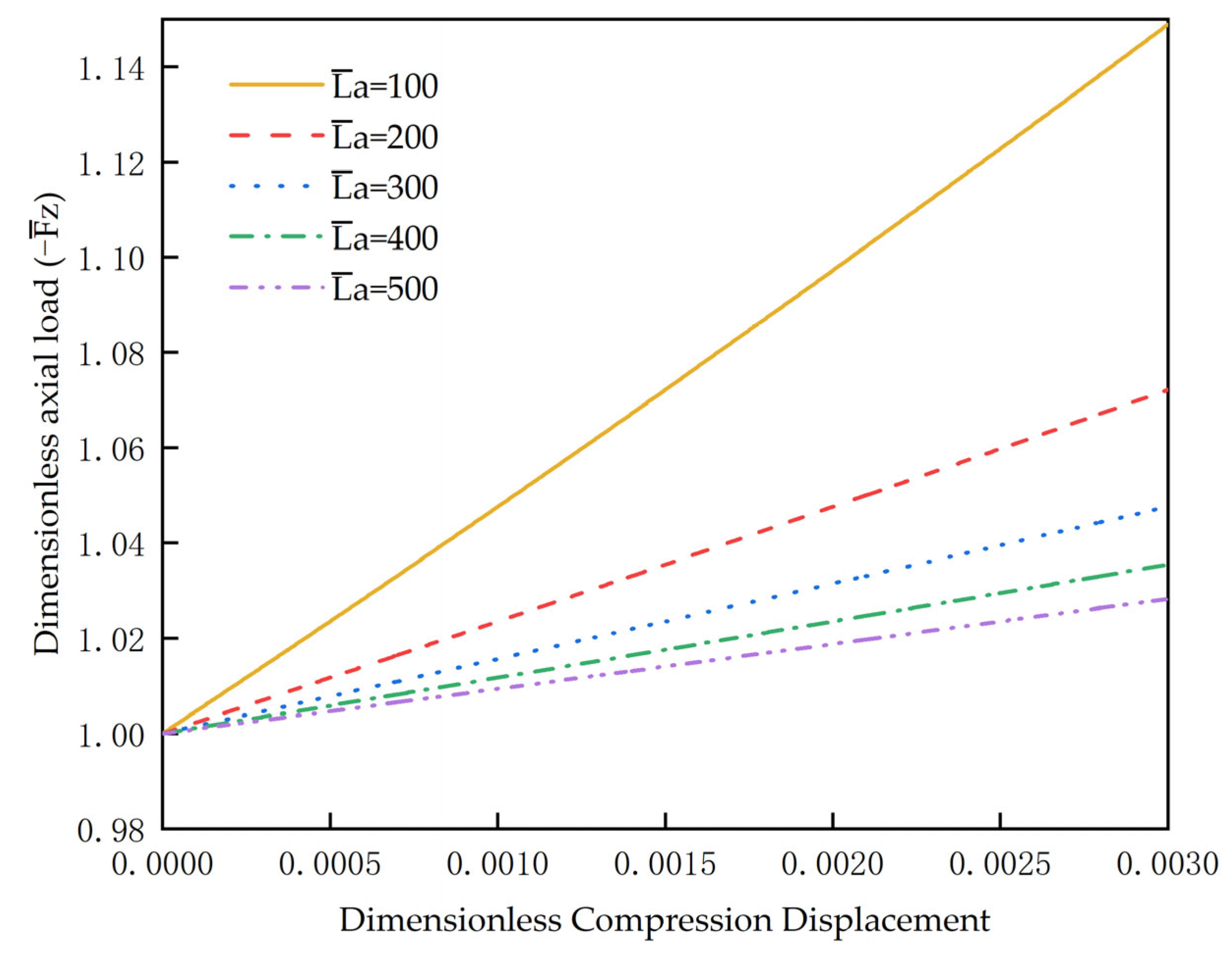
The critical load for sinusoidal buckling of the CT with a dimensionless length less than $\mathrm{4.7 }\pi$ is higher than Dawson’s model, when friction is ignored and the initial linear configuration is maintained. If the CT is long enough, the resulting half-wave number decreases as compression progresses during sinusoidal post-buckling. However, the sinusoidal half-wave number produced during the compression of shorter strings does not change at all.

(2)

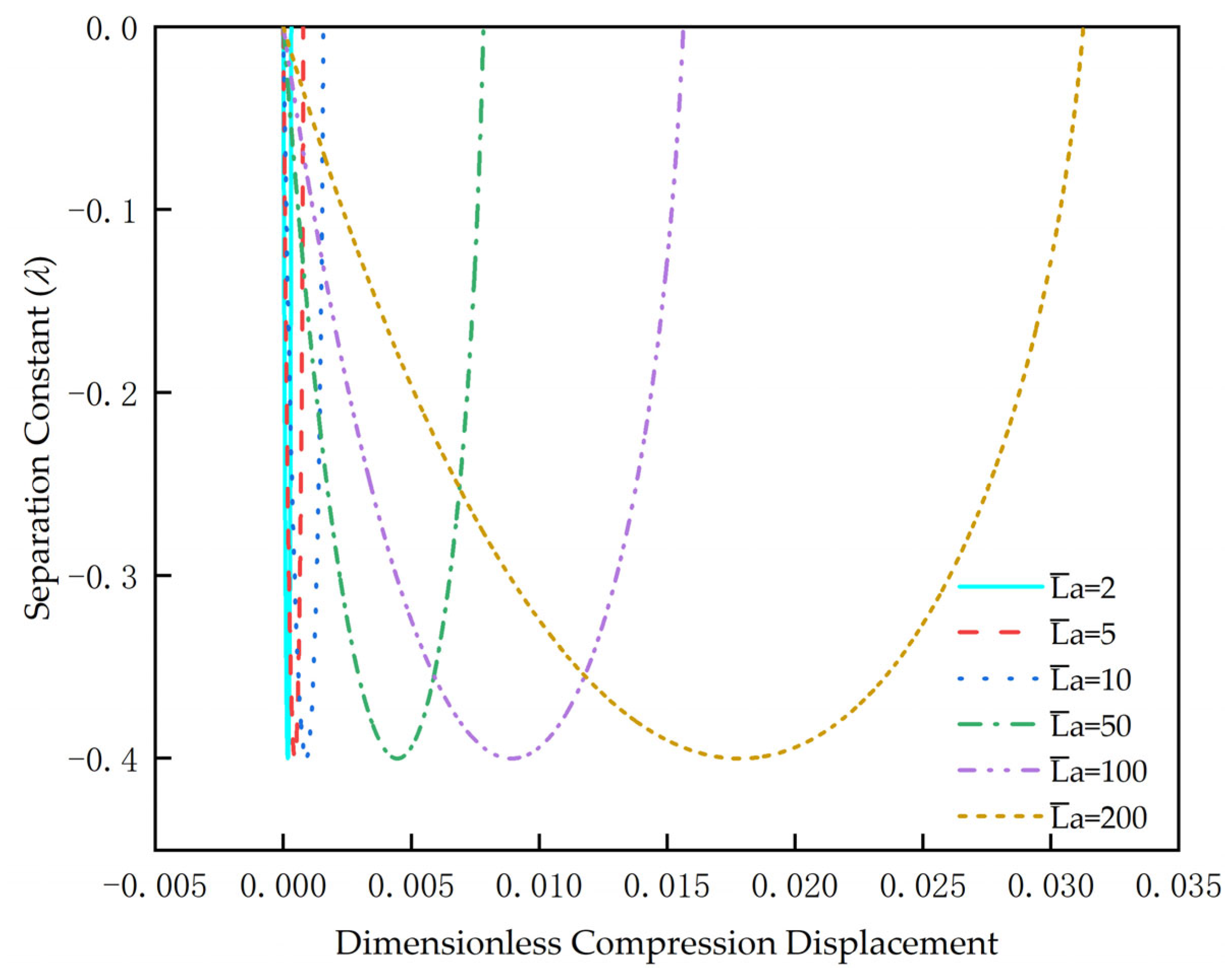
The range of the separation constant for CT under axial compression is $-0.4\le \lambda <0$, and sinusoidal buckling deformation is stable. As the compression continues, the critical value of stable deformation and unstable deformation is reached. At this point, the separation constant is equal to zero, the critical value is subjected to a dimensionless axial load value of approximately 1.876, and the string enters a mixed sinusoidal and helical buckling mode. This conclusion is basically consistent with 1.875 of Miska. The introduction of the separation constant method lays a foundation for the further study of the change process from sinusoidal buckling to spiral buckling.

(3)

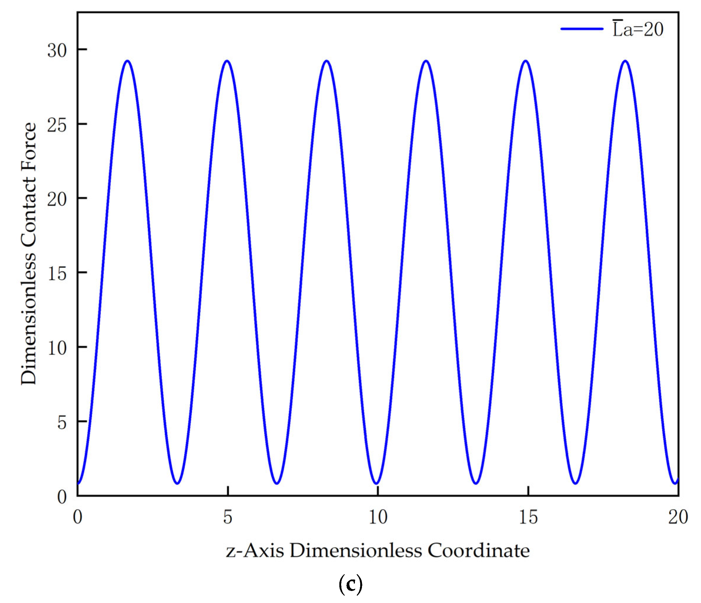
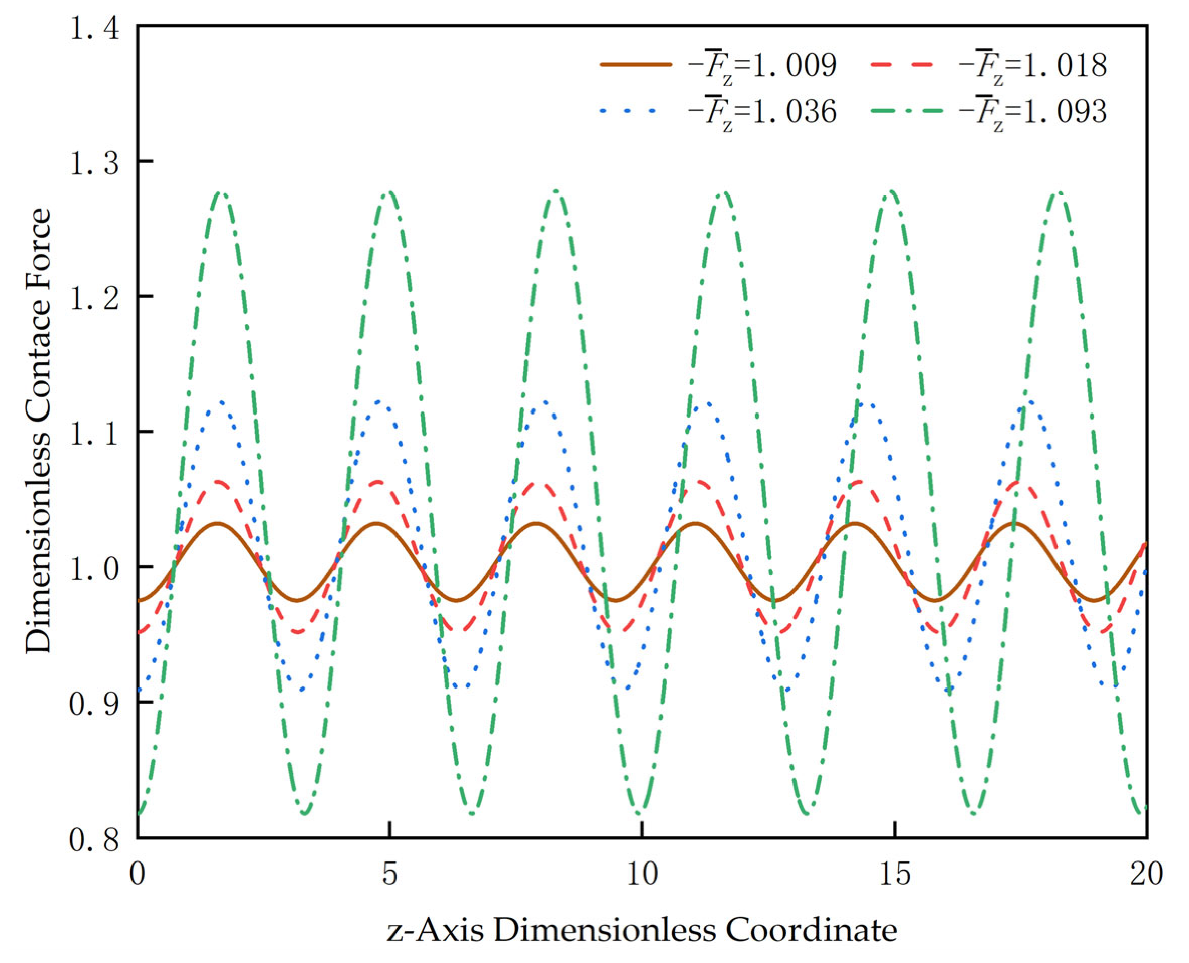
Based on the mathematical model of buckling, the contact force, including the dynamic term between the coiled tubing and the wellbore after sinusoidal buckling, is established. The change of the contact force on the wellbore wall when the coiled tubing moving at different speeds occurs sinusoidal buckling is numerically calculated. The results show that the greater the velocity, the greater the force on the wellbore. However, the force exerted on the wellbore by the string at the bottom of the horizontal well is basically unaffected by the velocity. It shows that the force generated by coiled tubing on the wellbore wall during the wellbore movement is greater than the theoretical calculation value of static string.

Mathematically, the set of differential equations for the buckling deformation of the coiled tubing is a system of high-order strongly nonlinear coupled system of partial differential equations, so the process of solving the equations uses a more idealized case, ignoring some boundary conditions such as friction, torque, and some small values. Although the compression distance at which the CT undergoes sinusoidal buckling is small, its deformation increases when the CT continues to be compressed, which may result in large errors if the small angle approximation in the paper continues to be used for analytical calculations. Therefore, the analysis process in this paper is limited to the process of sinusoidal buckling deformation of the CT. The future research will focus on the deformation state of the CT when the spiral buckling occurs using the mathematical model established in this paper, the effect of increasing the friction, torque and other boundary conditions on the mathematical model, and how the coiled tubing is converted from sinusoidal buckling to spiral buckling in the process of motion.

References

1. Mitchell, R.F. New buckling solutions for extended reach wells. In Proceedings of the IADC/SPE Drilling Conference, Dallas, TX, USA, 26 February 2002. [Google Scholar]
2. Mulcahy, C.G.; Su, T.X.; Wicks, N.; Reis, P.M. Extending the reach of a rod injected into a cylinder through axial rotation. J. Appl. Mech.-Trans. ASME 2016, 83, 051003. [Google Scholar] [CrossRef]
3. Miller, J.T.; Su, T.; Dussan, E.B.; Pabon, J.; Wicks, N.; Bertoldi, K.; Reis, P.M. Buckling-induced lock-up of a slender rod injected into a horizontal cylinder. Int. J. Solids Struct. 2015, 72, 153–164. [Google Scholar] [CrossRef]
4. Zhang, J.T.; Yin, G.F.; Li, Y.F.; Zhang, L. Buckling configurations of tubular strings constrained in three-dimensional curved wellbores. J. Pet. Sci. Eng. 2021, 195, 107953. [Google Scholar] [CrossRef]
5. Mitchell, R.F. Buckling behavior of well tubing: The packer effect. Soc. Pet. Eng. J. 1982, 22, 616–624. [Google Scholar] [CrossRef]
6. Paslay, P.R.; Bogy, D.B. The stability of circular rod laterally constrained to be in contact with an inclined circular cylinder. J. Appl. Mech.-Trans. ASME 1964, 31, 605–610. [Google Scholar] [CrossRef]
7. Dawson, R. Drilling pipe Bucking in Inclined Holes. J. Pet. Technol. 1984, 36, 1734–1738. [Google Scholar] [CrossRef]
8. Gao, D.L.; Huang, W.J. A review of down-hole tubular string buckling in well engineering. Pet. Sci. 2015, 12, 443–457. [Google Scholar] [CrossRef]
9. Hajianmaleki, M.; Daily, J.S. Advances in critical buckling load assessment for tubulars inside wellbores. J. Pet. Sci. Eng. 2014, 116, 136–144. [Google Scholar] [CrossRef]
10. Yu, Y.P.; Chen, L.H.; Sun, W.P.; Zeng, B.H.; Sun, Y.H. An analytical investigation on large post-buckling behavior of a drilling shaft modeled as a rotating beam with various boundary conditions. Int. J. Mech. Sci. 2018, 148, 486–495. [Google Scholar] [CrossRef]
11. Kuang, Y.C.; Lin, W.; Liu, Y.; Wang, Q.; Zhang, J.Z. Numerical modelling and field experimental validation of the axial load transfer on the drill-strings in deviated wells. J. Nat. Gas Sci. Eng. 2020, 75, 103124. [Google Scholar] [CrossRef]
12. Chen, Y.C.; Lin, Y.H.; Cheatham, J.B. Tubing and casing buckling in horizontal wells. J. Pet. Technol. 1990, 42, 140–191. [Google Scholar] [CrossRef]
13. Khodabakhsh, R.; Saidi, A.R.; Bahaadini, R. An analytical solution for nonlinear vibration and post-buckling of functionally graded pipes conveying fluid considering the rotary inertia and shear deformation effects. Appl. Ocean Res. 2020, 101, 102277. [Google Scholar] [CrossRef]
14. Qin, X.; Gao, D.L.; Huang, W.J. Frictional buckling analyses of slender rod constrained in a horizontal cylinder. Eur. J. Mech. A-Solids 2019, 76, 70–79. [Google Scholar] [CrossRef]
15. Huang, W.J.; Gao, D.L.; Wei, S.L.; Chen, P.J. Boundary condition: A key factor in tubular-string buckling. SPE J. 2016, 20, 1409–1420. [Google Scholar] [CrossRef]
16. Bang, J.; Jegbefume, O.; Ledroz, A.; Weston, J.; Thompson, J. Analysis and Quantification of Wellbore Tortuosity. SPE Prod. Oper. 2017, 32, 118–127. [Google Scholar] [CrossRef]
17. Matthews, C.M.; Dunn, L.J. Drilling and production practices to mitigate sucker rod/tubing wear-related failures in directional wells. SPE Prod. Fac. 1993, 8, 251–259. [Google Scholar] [CrossRef]
18. Mitchell, R.F. The effect of friction on initial buckling of tubing and flowlines. SPE Drill. Complet. 2007, 22, 112–118. [Google Scholar] [CrossRef]
19. He, X.J.; Kyllingstad, A. Helical buckling and lock-up conditions for coiled tubing in curved wells. SPE Drill. Complet. 1995, 10, 10–15. [Google Scholar] [CrossRef]
20. Zhu, Z.L.; Hu, G.; Fu, B.W. Buckling behavior and axial load transfer assessment of coiled tubing with initial curvature in constant-curvature wellbores. J. Pet. Sci. Eng. 2021, 195, 107794. [Google Scholar] [CrossRef]
21. Gao, G.H.; Miska, S. Effects of boundary conditions and friction on static buckling of pipe in a horizontal well. SPE J. 2009, 14, 782–796. [Google Scholar] [CrossRef]
22. Gao, G.H.; Miska, S. Effects of friction on post-buckling behavior and axial load transfer in a horizontal well. SPE J. 2010, 15, 1110–1124. [Google Scholar] [CrossRef]
23. Zhang, Q.; Wang, J.C.; Cui, W.; Xiao, Z.M.; Yue, Q.B. Post-buckling transition of compressed pipe strings in horizontal wellbores. Ocean Eng. 2020, 197, 106880. [Google Scholar] [CrossRef]
24. Gao, D.L. Down-Hole Tubular Mechanics and Its Applications, 1st ed.; China University of Petroleum Press: Dongying, China, 2006; pp. 16–42. [Google Scholar]
25. Huang, W.J.; Gao, D.L.; Liu, F.W. Buckling analysis of tubular strings in horizontal wells. SPE J. 2015, 20, 405–416. [Google Scholar] [CrossRef]
26. Li, Z.F.; Zhang, C.Y.; Song, G.M. Research advances and debates on tubular mechanics in oil and gas wells. J. Pet. Sci. Eng. 2017, 151, 194–212. [Google Scholar] [CrossRef]
27. Mitchell, R.F. New concepts for helical buckling. SPE Drill. Eng. 1988, 3, 303–310. [Google Scholar] [CrossRef]
28. Zhang, J.T.; Yin, G.F.; Fan, Y.; Zhang, H.L.; Tian, L.; Qin, S.; Zhu, D.J. The helical buckling and extended reach limit of coiled tubing with initial bending curvature in horizontal wellbores. J. Pet. Sci. Eng. 2021, 200, 108398. [Google Scholar] [CrossRef]
29. Liu, J.P.; Zhong, X.Y.; Cheng, Z.B.; Feng, X.Q.; Ren, G.X. Buckling of a slender rod confined in a circular tube: Theory, simulation, and experiment. Int. J. Mech. Sci. 2018, 140, 288–305. [Google Scholar] [CrossRef]
30. Miska, S.; Qiu, W.Y.; Volk, L.; Cunha, J.C. An Improved Analysis of Axial Force along Coiled Tubing in Inclined/Horizontal Wellbores; Society of Petroleum Engineers (SPE): Richardson, TX, USA, 1996. [Google Scholar]
31. Timoshenko, S.P.; Gere, J.M. Theory of Elastic Stability, 2nd ed.; Dover Publications, Inc.: Mineola, TX, USA, 2009; pp. 87–104. [Google Scholar]
32. Qin, X.; Gao, D.L.; Chen, X.Y. Effects of initial curvature on coiled tubing buckling behavior and axial load transfer in a horizontal well. J. Pet. Sci. Eng. 2017, 150, 191–202. [Google Scholar] [CrossRef]
33. Cunha, J.C. Buckling of tubulars inside wellbores: A review on recent theoretical and experimental works. SPE Drill. Complet. 2004, 19, 13–19. [Google Scholar] [CrossRef]
Figure 1. Schematic diagram of horizontal CT: (a) CT with sinusoidal buckling; (b) Coordinate parameters of CT section.
Machines 11 00563 g001
Figure 2. Relationship between CT with different lengths and critical load.
Machines 11 00563 g002
Figure 3. Relationship between axial load and amplitude.
Machines 11 00563 g003
Figure 4. Relation between the separation constant and square of the amplitude.
Machines 11 00563 g004
Figure 5. Relationship between Compression Displacement and Axial Load.
Machines 11 00563 g005
Figure 6. Relationship between Separation Constant and Compression Displacement.
Machines 11 00563 g006
Figure 7. The relationship between amplitude and half-wave number.
Machines 11 00563 g007
Figure 8. Contact force curves of CT with different lengths on the horizontal well wall: (a) The dimensionless length is equal to 5; (b) The dimensionless length is equal to 10; and (c) The dimensionless length is equal to 20.
Machines 11 00563 g008aMachines 11 00563 g008b
Figure 9. Contact force for different compression displacements.
Machines 11 00563 g009
Figure 10. Variation curves of contact force at different speeds.
Machines 11 00563 g010
Figure 11. Variation curves of contact force under different axial loads.
Machines 11 00563 g011