Abstract
Based on data-driven and mixed models, this study proposes a fault detection method for autonomous underwater vehicle (AUV) rudder systems. The proposed method can effectively detect faults in the absence of angle feedback from the rudder. Considering the parameter uncertainty of the AUV motion model resulting from the dynamics analysis method, we present a parameter identification method based on the recurrent neural network (RNN). Prior to identification, singular value decomposition (SVD) was chosen to denoise the original sensor data as the data pretreatment step. The proposed method provides more accurate predictions than recursive least squares (RLSs) and a single RNN. In order to reduce the influence of sensor parameter errors and prediction model errors, the adaptive threshold is mentioned as a method for analyzing prediction errors. In the meantime, the results of the threshold analysis were combined with the qualitative force analysis to determine the rudder system’s fault diagnosis and location. Experiments conducted at sea demonstrate the feasibility and effectiveness of the proposed method.
1. Introduction
The development of autonomous underwater vehicles (AUVs) over the past three decades has exhibited a high security, high controllability, and low cost [1]. AUVs are utilized extensively in hydrological surveys, seabed surveys, environmental assessments, and other fields today. Due to the complexity of and variation in the circumstances, it is difficult for AUVs to avoid all faults caused by events or the AUV itself [2]. As the primary source of motion control for AUVs, excluding the thrusters, the rudder is also the leading source of AUV malfunctions. In the event of rudder defects, the motion control of AUVs is compromised. Therefore, detecting rudder failure is critical to improving the safety of AUVs.
In recent years, the methods for detecting AUV faults have primarily incorporated three aspects: signal processing, an analytical model, and a data-driven model [3]. Enhanced fractal features integrated with the wavelet decomposition identification method were proposed for AUVs with a thruster fault, and the time-domain and frequency-domain data were utilized to identify thruster malfunctions [4]. In order to address the issue that there is no useful feature in the frequency domain, Yu et al. [5] proposed a new method for calculating the weak fault severity of thrusters’ features. Maleki et al. [6] devised the discrete wavelet transform as a method for monitoring machine vibrations and employed the DWT-FFT signal processing method to detect the fault of the rotating shaft. Signal processing techniques are widely utilized in rotating machinery fault detection [7], but, for AUVs, the signal processing technique is impacted by random ocean currents and intense measurement noise [8]. After signal processing, it is difficult to distinguish the fault feature from the disturbance feature for a weak fault [9]. As a result, the issue of incorrect diagnosis arises.
The analytical model-based implementation is relatively simple. Sun et al. [10] developed a fault diagnosis (FD) scheme based on a Gaussian particle filter (PF) and demonstrated the practicability and validity of the developed method for estimating the AUV failure model and motion state. In their study, Lv et al. [11] proposed a fault-tolerant control (FTC) method integrated with thrust allocation based on the sliding mode theory to reduce the error caused by thruster faults when using a conventional sliding mode controller. In order to solve the unknown effects of multiple autonomous underwater vehicles (AUVs) system actuator failures, Xu et al. [12] designed a fault-tolerant control method based on extended state observers (ESOs) and an adaptive strategy. Abdollahi [13] established a method that decouples the entire system into two subsystems and designed two independent sliding mode observers (SMOs) to estimate sensor and actuator faults for corresponding subsystems. A particle filter (PF)-based robust navigation system with FD was designed for an underwater robot [14]. A method for fault localization was proposed that calculated the pole-to-pole voltage as diagnostic variables and designed an error-based threshold [15]. Chu et al. [16] proposed an observer-based fault detection method for magnetically coupled undersea thrusters. Yin et al. [17] designed an FD method based on the current observer that used fault residuals to detect and locate faults and an adaptive threshold to reduce error interference. Due to the complexity of the ocean environment and other factors, it is difficult to create an accurate model [18]. In contrast, the model-based method is sensitive to system parameters and dependent on the traditional experience threshold, which reduces its robustness, and it also has stricter control system requirements [19].
The data-driven fault diagnosis methods do not require models. Compared to traditional model-based diagnosis, this method significantly reduced the time required for diagnosis and increased efficiency. An example of using recurrent neural networks (RNNs) is given by Nascimento and Valdenegro-Toro [20], who presented a data-driven fault detection and diagnosis scheme for underwater thrusters.
Fabiani et al. [21] presented a method for fault detection and isolation on the thrusters of an over-actuated AUV based on non-linear principal component analysis (NLPCA) and an off-line artificial neural network (ANN). Combined with motor current signals, Li et al. [22] proposed a new scheme based on a deep extreme learning machine for roller bearing fault diagnosis. Ji et al. [23] investigated a novel fault diagnosis method based on convolutional neural networks (SeqCNN). Although the data-driven fault diagnosis methods are accurate, their adaptability is weak [24].
Increasing numbers of FD studies employ a combination of signal processing and analytical model-based and data-driven approaches in order to ensure the accuracy of FD and improve the diagnostic feasibility. Chu et al. [25] developed an RBF neural-network-based adaptive sliding mode control scheme. The state space equation was used to describe the dynamic model of ROVs. When the propeller is saturated, this hybrid model approach combines a neural network and sliding mode control to ensure the stability of the adaptive trajectory tracking system. Wang et al. [26] designed a method for extracting features from raw vibration signals and used 1D-CNN-based networks for bearing FD, combining signal processing techniques with a data-driven approach. A fault-tolerant control method based on adaptive and radial basis function neural networks (RBFNN) was proposed by Wang et al. [27] for autonomous underwater vehicles exposed to dynamic uncertainties and potential unknown thruster failures. Xu et al. [28] designed a novel robust Gaussian approximation smoother based on the expectation–maximization (EM) algorithm, combining data-driven and model-building methods.
However, the majority of research on AUV FD has focused on thruster and sensor failures. Few studies have been conducted on the FD of AUV rudder systems, and the ones that have are frequently concerned with fault-tolerant control. Liu and Xu [29] addressed the issue of fault localization (FL) and fault-tolerant control (FTC) for AUV rudders when deformation faults occur. Liu et al. [30] were primarily concerned with the development of FTC based on active compensation in rudder fault mode. Che and Yu [31] designed two neural network estimators to estimate rudder faults and ocean current disturbance, respectively, to solve the fault-tolerant tracking control problem. However, the aforementioned methods were only validated through simulation. A PF-based method for estimating rudder effect deduction and the unscented Kalman filter (UKF) were proposed for proposal distribution, respectively [32]. By analyzing the pertinent indicators, the rudder’s fault type could be determined and experimentally confirmed; however, the current focus of this method is on the response of the AUV to the dynamics control under ideal conditions; the parameter error of the sensor was not considered, and the sensor’s usability must be enhanced.
This paper, inspired by prior research, presents a data-driven and hybrid-model FD scheme for the AUV rudder system. Given this, the following are the principal contributions of this paper.
- (1)
- Aiming at the fault problem of an AUV rudder without feedback, a new rudder fault detection method combined with an AUV dynamic model is proposed in this paper. Considering the uncertainty of AUV dynamic model parameters, this paper proposes an RNN-based method for identifying the nonlinear parameters of an AUV dynamic model. At the same time, the singular value decomposition (SVD) method was used to denoise the original data. Compared with the parameter identification methods based on RLS and the traditional RNN, the proposed method has a higher identification accuracy.
- (2)
- In order to reduce the influence of sensor parameter errors and prediction model errors on fault detection results, this paper developed an adaptive threshold for analyzing prediction results. Compared with the method of fault diagnosis based on an empirical threshold, the proposed method adapts to changes in environmental parameters and has a higher reliability, thereby reducing the incidence of misdiagnosis.
2. Problems Description
This section focuses primarily on the AUV rudder system and rudder faults.
2.1. Rudder System of AUV
The AUV rudder system consists of horizontal and vertical rudders, as shown in Figure 1. Included in horizontal rudders are the left and right rudders. The vertical rudders consist of the up rudder and the down rudder. The Sailfish-210 AUV’s rudder control system (Ocean University of China, Qingdao, China) includes electric rudders, a signal collection system, a power system, an industrial personal computer system, etc. As depicted in Figure 2, the AUV’s rudder control system is described in detail.
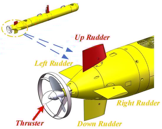
Figure 1.
Layout of cross-rudder and thruster in Sailfish-210 AUV.
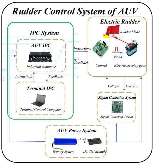
Figure 2.
Rudder control system of AUV.
Each electric rudder within the AUV comprises electric steering gear, a controller, and rudder mounting devices (including rudder blades). For collecting the rudder current, the signal acquisition system includes a sampling resistor, an operational amplifier, and a filter circuit. The IPC system includes both the AUV’s internal industrial computer and an industrial computer located on land. The industrial computer system serves as the AUV’s brain, controlling the delivery and acceptance of instructions. The power supply system supplies the AUV with power.
2.2. Problem Formulation
The rudder utilized by the AUV analyzed in this paper lacks angle feedback. Due to the rudder’s instability and external damage, the rudder may fail, resulting in a decrease in the AUV’s mobility. As an essential actuator for AUVs, rudder fault diagnosis is essential. In the fault mode of the AUV rudder system—for instance, where the expected rudder angle does not match the actual rudder angle, or where the rudder blade is damaged, etc.—it can be difficult to determine the cause. Combining the AUV’s pitch, roll, yaw angle, and other data is necessary to complete the rudder FD. We divided rudder fault types into the following categories:
- (1)
- The rudder blade falls off. Due to structural deterioration or external impact interference, the rudder blade detaches.
- (2)
- Rudder jam. The rudder becomes stuck in a fixed position, reducing maneuverability. This category of faults includes a stuck rudder gear, seaweed clogging the rudder shaft, etc.
- (3)
- Rudder blade deflection failure or rudder blade damage. The fault type of rudder blade deflection manifests itself when the expected rudder angle differs from the actual rudder angle as a result of the aging of the rudder blade and the decreased accuracy of the internal potentiometer, etc. In this article, the deflection fault type is set to a value greater than . Additionally, the effectiveness of the rudder will be diminished if the rudder blade is damaged by impact or scratches. This type of control surface damage resembles a deflection fault in its behavior. Consequently, no distinction will be made.
According to the degree of risk posed by various types of faults, fault types are classified into distinct fault levels. Then, the emergent operations corresponding to those in Table 1 are applied. In a real-world scenario, an accurate diagnosis is necessary to enable a more effective response to the occurrence of these faults and to ensure AUV safety [24].

Table 1.
Fault types and emergency operations.
3. Models and Algorithm
This section primarily establishes the method of model parameter identification, including the AUV dynamic model and RNN structure, as well as introducing the SVD, adaptive threshold methods, and algorithm flow.
3.1. Dynamic Model of AUV
According to the Society of Naval Architects and Marine Engineers (SNAME), the Earth-fixed frame and body-fixed frame are intended to characterize the 6-DOF dynamic equations of motion of an AUV. Figure 3 depicts the AUV’s appearance and two coordinate systems.
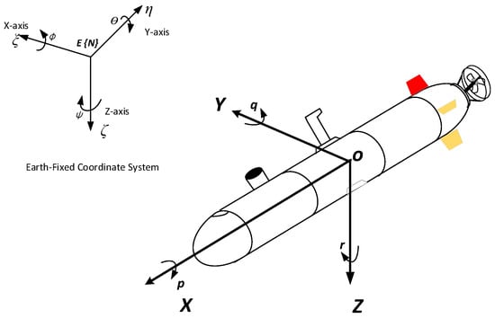
Figure 3.
The body-fixed and Earth-fixed coordinate systems of AUV.
According to [33], the transformation between the body-fixed frame and the Earth-fixed frame is as follows:
where denotes the vector of position and orientation in the Earth-fixed frame; is the transformation matrix; is the vector of velocity and angular velocity expressed in the body-fixed frame.
The dynamic equation for an AUV is given by:
where M denotes the inertia matrix; , and present the Coriolis-centripetal matrix, damping matrix, and vector of gravity forces, respectively; is described in frame respective to the linear and angular acceleration vectors; denotes the constant and time-varying disturbances induced by waves and ocean currents; is the vector of the control input. According to [34], the 6-DOF dynamic model of the AUV in (2) can be expanded as:
where , and are the sum of the components of the force and moment acting on the AUV; m is the mass of the AUV; denotes the center of gravity; , and represent inertial moments about the x, y, and z axes, respectively. represents the AUV speed in , , and . denotes the AUV angular velocity in , , and .
In the 6-DOF dynamic model, compared with the force equations, it is easier for the torque equations to reflect the internal relationship between the AUV attitude information and the rudder angle. We simplified the equations of motion and identified the system model parameters using the roll, pitch, and yaw moment equations. According to [35,36], the sum external moments of the AUV in (3) can be expanded as:
where , etc., represent the hydrodynamic coefficient. In order to describe the attitude information vividly, combining (3) and (4), the pitch angle, roll angle, and yaw angular acceleration can be expressed as [37,38]:
where and denote the vehicle’s pitch and roll angle, respectively; represents the yaw angular acceleration; parameters , and represent the weights of various variables. From (5), we can see that , and are determined by the thirteen, ten, or fourteen variables on the right side of the equation, respectively. These variables, with the exception of , and , are obtained directly from the AUV sensors. denotes the torque generated by the propeller about the X-axis, expressed as [39]:
where denotes the seawater density; is the torque coefficient; represents the propeller diameter; n represents propeller speed. , and represent the pitch, roll, and yaw torque generated by the rudder system in AUV coordinate system, respectively, expressed as [40,41]:
where denotes the speed of the vehicle, as shown in Figure 4; is the side projection area of the rudder blade; and represent the vertical rudder angle and horizontal rudder angle, respectively; L is the total length of the vehicle; , , , and are the position derivatives of the torque factors with respect to relevant rudder angles. Table 2 gives the parameters of the Sailfish-210 (Ocean University of China, Qingdao, China).
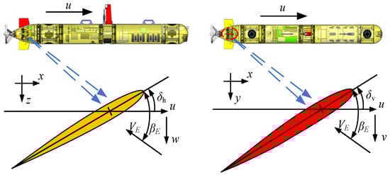
Figure 4.
Effective angle of attack of the horizontal rudders and vertical rudders (the left is the side view of the AUV, and the right is the top view).
Table 2.
Parameters of the Sailfish-210 AUV.
The actual AUV’s rudder angle control output can be described as follows (using the vertical rudder as an example):
where is the design control input and is the upper limit of the rudder angle, where the upper limit rudder angle of the Sailfish-210 AUV is set to 40°. When the rudder blade is in its original position, we define the rudder angle as 0°. For left and right rudders, the angle when the rudder is turned down is typically defined as negative and the angle when it is turned up is defined as positive. For up and down rudders, the angle defined when the rudder is turned to the left is negative, and the angle defined when the rudder is turned to the right is positive.
Thus, we converted the parameters , and to , , , , , , , and . The objective is to identify these parameter values. This paper proposes a data-driven method for parameter identification based on a recurrent neural network. The sensor values on the right-hand side of Equation (5) serve as the model’s input. The model’s output is the pitch, roll, and yaw angular accelerations. In order to improve the precision of parameter identification, the AUV’s normal-state data are used as training data. The collected data are divided into a training set and a test set, the model is constructed by learning from the training set, and then its performance is evaluated using the test set. Considering the convergence speed of the LSTM network, a normalization approach is used to pre-process the data for the work. The iterative training process of the AUV pose motion model is evaluated with a loss function based on the known relationships of the discrimination system parameters to obtain an AUV system model with a high discrimination accuracy. This process of parameter identification is illustrated as a flow chart in Figure 5.
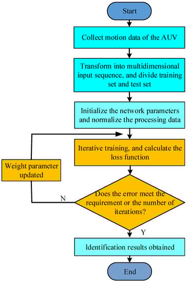
Figure 5.
Parameter identification process based on neural network.
3.2. RNN Structure
In this section, the parameter identification method is designed for the system equations of the previous subsection. There are more methods for parameter identification; for example, the least squares method and the maximum likelihood method [42]. In contrast to these two methods, neural networks with nonlinear mapping capability are selected to identify the parameter of this system. The neural-network-based parameter identification method aims to obtain a system equivalent to the theoretical model and is not concerned with the actual dynamical parameters in the AUV model. It avoids using much test data as training sample space in the identification process. The comparisons of specific methods are described in later sections.
A recurrent neural network (RNN) is a technology for deep learning designed to process time-series data. However, it is well known that classical RNNs have problems with long-range dependencies, which cause gradients to explode or vanish during backpropagation. The success of RNNs with LSTM cells in capturing long-term dependencies within a sequence has led to their increased prevalence in prediction applications. As shown in Figure 6, LSTM was selected for use in our framework based on its superior performance. The RNN-LSTM network cell can be represented as follows [43]:
where , , , and represent the input, forget, output gate, and memory cell, respectively. They are called gates because they are zero-valued sigmoid functions. Once trained, the RNN-LSTM has the advantage of a lower computational overhead [44]. The RNN-LSTM can solve the problem of long-term dependency. Due to these advantages, RNN-LSTM is an excellent candidate for identifying AUV model parameters.
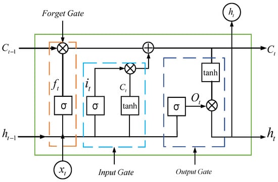
Figure 6.
The structure of the LSTM neural network.
Figure 7 depicts the architecture of neural networks used in this paper when combined with AUV sensors and actuators.
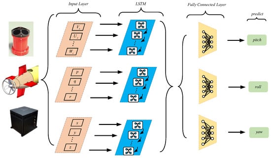
Figure 7.
Architecture of neural networks (here, “pitch” and “roll” represent the pitch and roll angles, respectively, and “yaw” represent yaw angular acceleration, not actual yaw angle).
In Figure 7, the input layer mainly imports the AUV velocity information obtained by the Doppler velocity log (DVL) and the attitude and heading reference system (AHRS), as well as the main thruster thrust and rudder angle in the motion control system. Using LSTM to build a prediction model, the number of LSTM network layers significantly impacts the speed and efficiency of training. Although the number of hidden layers will improve the training effect, too many will reduce the prediction accuracy and increase the time consumption. Considering the actual needs of the training time and the AUV model, this paper used a single LSTM network hidden layer. The full connected layer is mainly responsible for the dimensional transformation of the output information of the LSTM layer and the retention of useful AUV state characteristic information. Finally, the regression output layer takes the predicted AUV pitch, roll, and yaw information as the LSTM model output. Based on the above, the main parameters of the LSTM network are set as shown in Table 3:
Table 3.
The setting value of the LSTM parameter.
3.3. Data Denoising Algorithm
Noise will inevitably interfere with the generation, acquisition, and transmission of AUV sensor signals, necessitating denoising signal processing. The singular value decomposition is widely utilized in signal denoising due to its excellent trend-extracting properties [45]. Firstly, represents original input data, and is converted to a matrix X that is made up of L-dimensional vector .
where L is the window length and . L nonnegative eigenvalues are obtained via singular value decomposition. The first R larger eigenvalues typically reflect the signal’s primary energy, whereas the remainder are considered noise components. Consequently, the initial input signal can be described as follows:
where represents the primary signal component, represents the noise components, and represents the components represented by their singular values. The SVD includes two crucial parameters, the window length L and the reconstructed singular value R, which have a significant impact on the effect of denoising. Based on the results of the experiment, the window length L was set to 12 and the number of reconstructed singular values was set to 6.
3.4. Adaptive Threshold Method
The adaptive threshold generally means that the threshold of the system can be adjusted according to the changes in itself and the environment [46]. In this design, the AUV adaptive threshold consists of two parts: the error from the identification model and the error from the sensor accuracy.
A model identification error prevents the convergence of the prediction error to zero. Model identification errors are caused by numerous factors, such as thrust model errors, dynamic modeling uncertainty, and ocean current disturbance [47]. It is undeniable that this method has a strong prediction effect. The error fluctuates within a small range around 0 as a result of the effect of prediction and, after analysis, it approximates the normal distribution. The analysis process is shown in Algorithm 1.
| Algorithm 1 Analysis process for normal distribution |
| Require: prediction error sequence . |
| (The goodness-of-fit test for normal distribution). |
| If and then |
| Assume that it follows a normal distribution. |
| else |
| Assume that it does not follow a normal distribution. |
| end if |
denotes prediction error sequence. The standard deviation of prediction error can be expressed as:
where represents the mean of the prediction error and N is the number of errors. In order to express the actual size of the prediction error over a long period of time and reduce the likelihood of significant errors, we employed the confidence interval method [48,49]. We extracted the sequence of prediction errors from the trained model, set the confidence level to , and solved the confidence interval as . At a confidence level of , z is . The is close to 0; hence, we can set the adaptive threshold for the prediction model error as .
In addition to the error of the trained prediction model, the sensor parameter error must also be considered. Without considering the prediction model error, represents the input parameters of the system, whereas denotes the output of the system. Due to unavoidable measurement, noise, and other error factors, the input parameters contain some error, expressed by . The value of the error is usually related to X, and the relationship can be obtained from the sensor manual. Essentially, this relationship often depends on the accuracy error of the sensor itself. Take the motion speed error obtained by the DVL device used by the AUV in the experiment as an example, where its speed error is of the speed. When u represents the DVL speed value, the corrected output caused by the DVL speed error is . Therefore, the output of the system y should be corrected to .
According to the Taylor formula, the higher-order terms with smaller values are ignored, and only the terms below the second order are retained; thus, the following can be determined:
Therefore, the maximum error of the output, , can be expressed as follows:
3.5. Fault Detection Method
This paper primarily diagnoses three types of rudder faults and combines the monitoring of rudder current characteristics with the model prediction process.
3.5.1. The Fault Type of Rudder Jam
Rudder jam is a type of fault that directly affects maneuverability and may significantly harm the AUV. This type of error is frequently evaluated based on the rudder current. When the rudder receives the rotation signal, the rudder angle changes abruptly, and the rudder’s start current is significantly larger than usual. When no external load is present, the rudder current is minimal. When the rudder jam fault occurs, the rudder current rises to the rudder jam current value until the external blocking force is no longer present. The rudder jam fault can be diagnosed using this characteristic. According to the product manual, the Sailfish-210 AUV’s rudder current can reach up to 2.5 A.
3.5.2. The Fault Type of Rudder Blade Falls Off
When the rudder blade falls off, the situation is comparable to the current-based evaluation of a rudder blocking fault. Once the rudder blade falls off during an AUV sea test, no load is applied to the rudder and the current is minimal.
3.5.3. The Fault Type of Rudder Blade Deflection
This type of rudder fault is the most prevalent. This type of fault lacks notable current abnormality characteristics. Frequently, it is necessary to make decisions using the prediction model method proposed in this paper. First, to precisely locate the faulty rudder of the AUV, a qualitative force analysis must be performed on the faulty rudder. The vertical rudders work collaboratively to generate and , where angles and correspond to the inputs of the up and down vertical rudders, respectively. A fault on a vertical rudder may bring multidimensional faulty influences to and ; that is,
where and denote the vertical rudders and horizontal rudders, respectively; , , and are position derivatives of the torque factors with respect to relevant rudder angles. The horizontal rudders work collaboratively to generate and , where the angles of and correspond to the inputs of the right and left horizontal rudders, respectively. A fault on a horizontal rudder may bring multidimensional faulty influences to and ; that is,
In the rudder blade deflection mode of the AUV, the rudder blade is manifested to be offset at the expected angle, which adds additional force/torque to the AUV’s movement and affects the pitch, roll, and heading information. The additive fault factors may be expressed as follows:
where and represent the force/torque generated by the fault rudder angle of the AUV, respectively. According to (3), and have the same polarity; and have the same polarity; have the same polarity with . Therefore, only the polarities of the deflection moment , , and are represented here, and the details are shown in Table 4.
Table 4.
The polarities of rudder fault force (moment).
According to Table 4, it can be concluded that the deflection of the horizontal rudders has an apparent effect on the pitch angle and roll angle; the pitching moment variation can usually be ignored, so only the pitch and roll angle errors must be evaluated when diagnosing this fault type. The deflection of vertical rudders appears to have an effect on the yaw angle velocity and roll angle; the yaw moment can be disregarded, so only the pitch angle and yaw angle velocity errors must be evaluated when diagnosing such faults.
3.6. Algorithm Flow
The experiment’s algorithm flow chart is arranged as shown in Figure 8. Currently, this paper discusses the design of non-real-time system algorithms and focuses primarily on AUV experiment historical data.
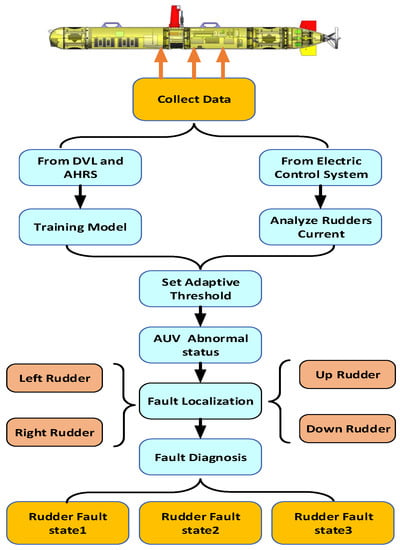
Figure 8.
The algorithm flow chart of the experiment.
4. Experiments and Results Analysis
This section mainly introduces the experimental platform, model identification results, and fault detection results.
4.1. Experimental Platform
Experiments on the AUV Sailfish-210, which was independently designed by the Ocean University of China and depicted in Figure 9a, were conducted to test the efficacy of the fault detection method proposed in this paper. Notably, although the algorithm is based on offline historical data, the data collected are real. All experimental data presented in this article originated from the Sailfish-210 AUV. Figure 9b depicts the Sailfish-210 AUV conducting a sea test.
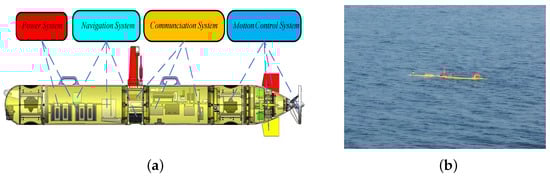
Figure 9.
Experimental platform: (a) the Sailfish-210 AUV prototype and systems; (b) the Sailfish-210 AUV is conducting a sea test.
4.2. Model Identification Results
In order to obtain stable motion data of AUV and verify the accuracy of the proposed parameter identification method, sea areas with a small current and good sea conditions were selected for the experiment. Through neural network training, the predicted value was obtained. This model training used the data between 0 and 150 s as the training set and the data between 384 and 451 s as the test set.
Figure 10 depicts the predicted effects of pitch, roll, and yaw acceleration. The parameter-identified error prevents the convergence of the value of the prediction error to zero. For fault-free modes, the prediction error occasionally exceeds the range of the adaptive threshold. We employed a 5 s time-window approach and tended to disregard short-term outliers. After calculation, the determination coefficients of the three predictions based on this method are , , and , respectively. This is a model with a high degree of dependability. The forecast error sequence has standard deviations of , , and .
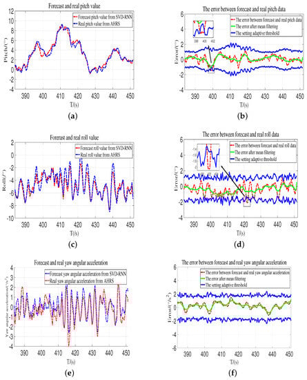
Figure 10.
Model training effect for pitch angle, roll angle, and yaw angular acceleration. (a) Forecast and real pitch value. (b) The error between forecast and real pitch data. (c) Forecast and real roll value. (d) The error between forecast and real roll data. (e) Forecast and real yaw angular acceleration. (f) The error between forecast and real yaw angular acceleration.
In order to further validate the efficacy of the proposed method, prediction results generated by recursive least squares (RLSs) and recurrent neural networks (RNNs) were compared with the proposed method. The RLS-based AUV model parameter identification method appeared earlier and has the advantages of fast and efficient identification, but it also has the problem of data saturation [50]. The RLS parameter identification method often obtains unsatisfactory results for AUV nonlinear factors. Neural networks for parameter identification do not care about the size of the parameters while looking for a good fit. The RNN neural network is improved from the traditional BP neural network. In this problem, the RNN network was chosen because of the poor training effect of BP. The superiority of RNN is that the concept of a time sequence is added to the network, which can learn, and the training effect is improved. However, the disadvantage is that the traditional RNN has the phenomenon of gradient explosion and disappearance [44].Therefore, an improved RNN method, LSTM, was adopted in this paper. Meanwhile, the singular value decomposition method deals with noise effects. As demonstrated in Figure 11, the pitch angle prediction results based on SVD-RNN are closer to the sensor’s original values.
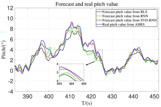
Figure 11.
Comparison of different methods for predicting pitch angle.
In this paper, in order to measure the performance of the prediction models, MAE and RMSE were selected as the evaluation indexes for the model’s prediction accuracy [51]. The formulas of these indexes are as follows:
where respects the actual values, respects the predicted values, and n is the amount of data forecasting.
Here, only the comparison of prediction effects of the pitch angle is listed in Figure 11. The comparison of prediction results of different methods of the roll angle and yaw data are similar to it, and no further graphical comparison is made. After a large number of training tests, the comparison between the model prediction by different methods and the original model according to the evaluation indicators is shown in Table 5.
Table 5.
Comparison of proposed methodology with RLS and RNN.
As can be seen from the comparison results, for the pitch angle predicted by the proposed method, compared with the prediction results using RLS and RNN, MAE is reduced by and , respectively, and RMSE is reduced by and , respectively. For the roll angle, MAE decreases by and , respectively, and RMSE decreases by and , respectively. For the yaw data, MAE is reduced by and , respectively, and RMSE is reduced by and , respectively. It can be seen that the MAE and RMSE of the prediction error using the proposed method are significantly reduced compared with RLS and RNN.
The above results reveal that the identification model is convergent and bounded, indicating that the proposed identification method is effective.
4.3. Fault Detection Results
In this subsection, several cases relating to different faults are carried out in order to verify the proposed fault detection method.
4.3.1. Experiment of Rudder Jam Fault
Figure 12 reveals that, at 35 s, the rudder current is close to the locked-rotor current, and the duration exceeds the predetermined threshold of 2 s. This fault is referred to as a rudder jam fault.
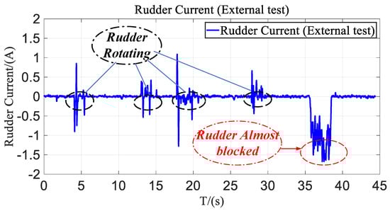
Figure 12.
The rudder current during rudder jam from external test.
4.3.2. Experiment of Rudder Blade Falling off Fault
Figure 13 shows that only at the rudder start time is there a large current, close to 1 A, whereas, for the rest of the time, the current is nearly zero. Consequently, this fault type is diagnosed as a rudder blade falling off.
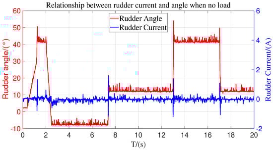
Figure 13.
The AUV rudder current when rudder blade falls off.
The fault diagnosis method for the rudder blade falling off and rudder jamming is mainly used to collect current information through the current module designed in the AUV cabin. This method is unsuitable for diagnosing rudder blade deflection faults because this fault type has no prominent current characteristics. Therefore, this fault diagnosis must be combined with the model method described above.
4.3.3. Experiment of Rudder Blade Deflection Fault
In the deflection fault experiments, different deflection angles of the rudder blade will have different effects on the model prediction residual. The actual rudder angle range of the AUV is and, if the rudder blade deflection angle is less than 5° or even smaller, the predicted residual is indeed very small, which will make judging the occurrence of faults difficult. Therefore, in this experiment, combined with the actual fault situation of the AUV, the fault type was set as the deflection angle of 15°, which is obvious enough for realizing the diagnosis and location of the rudder deflection fault.
Figure 14 depicts the effect predicted by the model when the right rudder is deflected downward by 15°.
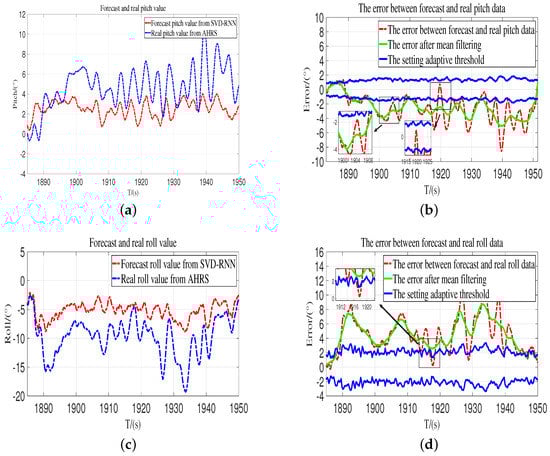
Figure 14.
Model training effect when the right rudder has downward deflection. (a) Forecast and real pitch value. (b) The error between forecast and real pitch data. (c) Forecast and real roll value. (d) The error between forecast and real roll data.
In this fault mode, the MAE and RMSE of the pitch angle prediction results are 2.237 and 2.918, and those of the roll angle prediction results are 5.286 and 6.849, respectively. The actual pitch value is greater than the value predicted by the model, the predicted roll value is obviously greater than the actual roll value (calculated in absolute value), and the error is significantly greater than the threshold value. In other words, the fault rudder produces undesirable roll and yaw torque and adversely affects the control process. As can be seen from Figure 14b,d, the prediction error lies within the set adaptation range at the moment close to 1920 s. The actual set failure duration threshold is 5 s, so it is determined that this phenomenon cannot be diagnosed as a normal state of the AUV rudder. This phenomenon is often caused by anomalous phenomena, such as the AUV suddenly receiving wave interference. Considering that this phenomenon is transient and does not occur frequently, this abnormal prediction result can be ignored.
According to the results of adaptive threshold analysis, the pitch and roll angle prediction errors of and in the fault mode are outside the range of the adaptive threshold, respectively, which proves that the method has a high accuracy. In order to illustrate the superiority of the method, it was compared with the commonly used RLS with the empirical threshold method, as shown in Figure 15. Based on historical experience reference, the threshold for this method was chosen to be 2°. The fault diagnosis accuracy of these two methods is shown in Table 6.
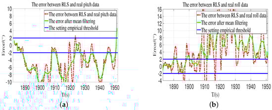
Figure 15.
The errors between the RLS model and real data from AHRS when the right rudder has downward deflection. (a) The error between the RLS model and real pitch data. (b) The error between the RLS model and real roll data.
Table 6.
Comparison of fault diagnosis accuracy of different methods when the right rudder has downward deflection.
Compared with the RLS with the empirical threshold method, the proposed method can improve the diagnostic accuracy by 18.1% and 40.7%, respectively, using the predicted pitch and roll results. Based on the results of the threshold analysis, the rudder is faulty. In order to diagnose this fault as a right rudder deflection fault, we refer to Table 4. The left rudder’s fault detection method is similar to that of the right rudder, and other types of horizontal rudder deflection will not be described in detail.
Figure 16 depicts the effect predicted by the model when the down vertical rudder is deflected leftward. This fault test was also carried out under the condition that the deflection angle is set to 15°.
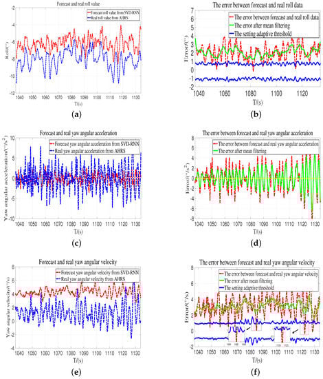
Figure 16.
Model training effect when the down rudder has leftward deflection. (a) Forecast and real roll data. (b) The error between forecast and real roll data. (c) Forecast and real yaw angular acceleration. (d) The error between forecast and real yaw angular acceleration. (e) Forecast and real yaw angular velocity. (f) The error between forecast and real yaw angular velocity.
As shown in Figure 16a,b, the predicted value of the roll angle by the model deviates significantly from the actual sensor value after 1885 s, and the error exceeds the adaptive threshold for an extended period. Figure 16c,d reveal that the prediction error of the yaw angular acceleration tends to fluctuate frequently, which makes it difficult to depict the yaw effect caused by the defective rudder accurately. In order to represent the change in the yaw moment more accurately, the yaw angular acceleration was converted to the yaw angular velocity using the following formula:
where represents the yaw angular acceleration and denotes the corresponding initial yaw angular velocity. The yaw rate is shown in Figure 16e,f. The actual yaw rate value is less than predicted by the model, and the error exceeds the adaptive threshold. In this failure case, the MAE and RMSE of the predicted results of the roll angle are 2.369 and 2.836, respectively; the MAE and RMSE of the predicted results of the yaw angular velocity are 3.240 and 4.037, respectively.
In this fault mode, and of roll and yaw angular velocity prediction errors are outside the adaptive threshold, respectively, which proves that the method has a high accuracy. Similar to the analysis of the left rudder fault results, in order to illustrate the superiority of the method, it was compared with the commonly used RLS with the empirical threshold method, as shown in Figure 17. The fault diagnosis accuracy of these two methods is shown in Table 7.
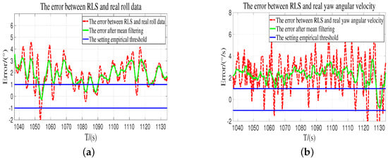
Figure 17.
The errors between the RLS model and real data from AHRS when the down rudder has leftward deflection. (a) The error between the RLS model and real roll data. (b) The error between the RLS model and real yaw angular velocity data.
Table 7.
Comparison of fault diagnosis accuracy of different methods when the down rudder has leftward deflection.
Compared with the RLS with the empirical threshold method, the proposed method can improve the diagnostic accuracy by 10.1% and 18.5%, respectively, using the predicted roll and yaw angular velocity results. This result shows that the proposed method has a specific advanced performance. According to the predicted results of the roll and yaw angular velocity, the down rudder is the type of fault that deflects to the left. It can be observed that the prediction error occasionally falls within the threshold range for the failure mode, and the AUV anomaly is responsible for this occurrence. Based on the sliding window method, it is determined that this phenomenon is typically brief and infrequent, so such anomalous prediction results can be disregarded. Other fault types of vertical rudders will not be discussed in detail.
In order to better support the effectiveness of the algorithm, we added a comparison of turning radius data under the AUV rudder fault mode, as shown in Figure 18. This fault test occurs when a part of the rudder force is lost in the down vertical rudder. It is also the deflection fault experiment shown in Figure 16. With the rudder angle set to 45° in normal mode, the fault deflection angle is set to −15°, which means that the down rudder angle after a fault is 30°. It can be seen from Figure 18 that the turning motion of the AUV is not precisely circular, which is caused by the disturbance of waves and other factors. After an approximate calculation, the turning radius of the AUV in the fault-free mode is approximately 25 m, whereas, in the fault mode, the turning radius of the AUV is approximately 15 m. This result indicates that the turning radius in the fault mode is much larger than that in the fault-free mode. The result also shows the rationality of using the AUV yaw angular velocity prediction results for fault diagnosis in yaw fault experiments.
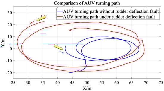
Figure 18.
Comparison of turning radius data under the AUV rudder fault mode.
The above experimental results indicate that, in the mode of rudder failure, the error between the predicted value of the model and the actual value of the sensor exceeds the adaptive threshold range, indicating that the proposed method is effective.
5. Conclusions
In this paper, the method for detecting rudder faults on an AUV in a marine environment was examined. This paper proposes an RNN-based method for identifying the nonlinear parameters of an AUV dynamic model using the trained model to predict the AUV’s attitude information. SVD was used to preprocess the training data to improve the accuracy of the model. In the meantime, an adaptive threshold method was developed to analyze the error between model predictions and actual sensor values, thereby enhancing FD precision.
This paper examined the common types of rudder deflection failure observed in AUV experiments. The experimental results confirm that the proposed method for fault detection is effective. Nevertheless, misdiagnosis may occur when relying solely on the adaptive threshold; the fault detection accuracy must be enhanced. In the normal rudder mode, a large roll angle or pitch angle can occur occasionally. Our future research will also focus on reducing these factors and enhancing the control performance of autonomous underwater vehicles. In this paper, data-driven and hybrid model methods were proposed to prepare for the future FD and FTC of rudders.
Author Contributions
Conceptualization, Z.Z.; methodology, Z.Z. and S.G.; software, Z.Z.; validation, Z.Z. and S.G.; formal analysis, Z.Z. and Z.Y.; investigation, X.Z.; resources, X.Z.; data curation, Z.Z.; writing—original draft preparation, Z.Z.; writing—review and editing, X.Z., T.Y., S.G. and Z.Y.; visualization, S.G. and Z.Y.; supervision, X.Z. and T.Y.; project administration, X.Z. and T.Y.; funding acquisition, X.Z. All authors have read and agreed to the published version of the manuscript.
Funding
This work was supported by the National Key Research and Development Program of China (Grant No. 2016YFC0301400).
Institutional Review Board Statement
Not applicable.
Informed Consent Statement
Not applicable.
Data Availability Statement
Not applicable.
Conflicts of Interest
The authors declare no conflict of interest.
References
- Yu, C.M.; Lin, Y.H. Experimental Analysis of a Visual-Recognition Control for an Autonomous Underwater Vehicle in a Towing Tank. Appl. Sci. 2020, 10, 2480. [Google Scholar] [CrossRef]
- Cui, R.; Yang, C.; Li, Y.; Sharma, S. Adaptive neural network control of AUVs with control input nonlinearities using reinforcement learning. IEEE Trans. Syst. Man Cybern. Syst. 2017, 47, 1019–1029. [Google Scholar] [CrossRef]
- Xia, S.; Zhou, X.; Shi, H.; Li, S.; Xu, C. A fault diagnosis method based on attention mechanism with application in Qianlong-2 autonomous underwater vehicle. Ocean Eng. 2021, 233, 109049. [Google Scholar] [CrossRef]
- Liu, W.; Wang, Y.; Yin, B.; Liu, X.; Zhang, M. Thruster fault identification based on fractal feature and multiresolution wavelet decomposition for autonomous underwater vehicle. Proc. Inst. Mech. Eng. Part J. Mech. Eng. Sci. 2017, 231, 2528–2539. [Google Scholar] [CrossRef]
- Yu, D.; Zhu, C.; Zhang, M.; Liu, X. Experimental Study on Multi-Domain Fault Features of AUV with Weak Thruster Fault. Machines 2022, 10, 236. [Google Scholar] [CrossRef]
- Maleki, Y.K.; Safizadeh, M.S.; Khajavi, M.N.; Payganeh, G.; Shuruni, S. Over hang slant cracked rotor vibration signal processing based on discrete wavelet transform. In Proceedings of the 2016 13th International Multi-Conference on Systems, Signals & Devices (SSD), Leipzig, Germany, 21–24 March 2016; pp. 672–676. [Google Scholar]
- Lu, S.; He, Q.; Wang, J. A review of stochastic resonance in rotating machine fault detection. Mech. Syst. Signal Process. 2019, 116, 230–260. [Google Scholar] [CrossRef]
- Li, J.; Du, J.; Zhu, G.; Lewis, F.L. Simple adaptive trajectory tracking control of underactuated autonomous underwater vehicles under LOS range and angle constraints. IET Control Theory Appl. 2020, 14, 283–290. [Google Scholar] [CrossRef]
- Lv, T.; Chen, Z.; Yao, F.; Zhang, M. Fault feature extraction method based on optimized sparse decomposition algorithm for AUV with weak thruster fault. Ocean Eng. 2021, 233, 109013. [Google Scholar] [CrossRef]
- Sun, Y.S.; Ran, X.R.; Li, Y.M.; Zhang, G.C.; Zhang, Y.H. Thruster fault diagnosis method based on Gaussian particle filter for autonomous underwater vehicles. Int. J. Nav. Archit. Ocean. Eng. 2016, 8, 243–251. [Google Scholar] [CrossRef]
- Lv, T.; Zhou, J.; Wang, Y.; Gong, W.; Zhang, M. Sliding mode based fault tolerant control for autonomous underwater vehicle. Ocean Eng. 2020, 216, 107855. [Google Scholar] [CrossRef]
- Xu, J.; Cui, Y.; Xing, W.; Huang, F.; Yan, Z.; Wu, D.; Chen, T. Anti-disturbance fault-tolerant formation containment control for multiple autonomous underwater vehicles with actuator faults. Ocean Eng. 2022, 266, 112924. [Google Scholar] [CrossRef]
- Abdollahi, M. Simultaneous sensor and actuator fault detection, isolation and estimation of nonlinear Euler-Lagrange systems using sliding mode observers. In Proceedings of the 2018 IEEE Conference on Control Technology and Applications (CCTA), Copenhagen, Denmark, 21–24 August 2018; pp. 392–397. [Google Scholar]
- Zhao, B.; Skjetne, R.; Blanke, M.; Dukan, F. Particle filter for fault diagnosis and robust navigation of underwater robot. IEEE Trans. Control Syst. Technol. 2014, 22, 2399–2407. [Google Scholar] [CrossRef]
- Li, Z.; Ma, H.; Bai, Z.; Wang, Y.; Wang, B. Fast transistor open-circuit faults diagnosis in grid-tied three-phase VSIs based on average bridge arm pole-to-pole voltages and error-adaptive thresholds. IEEE Trans. Power Electron. 2017, 33, 8040–8051. [Google Scholar] [CrossRef]
- Chu, Z.; Chen, Y.; Zhu, D.; Zhang, M. Observer-based fault detection for magnetic coupling underwater thrusters with applications in jiaolong HOV. Ocean Eng. 2020, 210, 107570. [Google Scholar] [CrossRef]
- Yin, H.; Chen, Y.; Chen, Z. Observer-based adaptive threshold diagnosis method for open-switch faults of voltage source inverters. J. Power Electron. 2020, 20, 1573–1582. [Google Scholar] [CrossRef]
- Lyu, P.; Liu, S.; Lai, J.; Liu, J. An analytical fault diagnosis method for yaw estimation of quadrotors. Control Eng. Pract. 2019, 86, 118–128. [Google Scholar] [CrossRef]
- Yin, H.; Chen, Y.; Chen, Z.; Li, M. Adaptive Fast Fault Location for Open-Switch Faults of Voltage Source Inverter. IEEE Trans. Circuits Syst. I Regul. Pap. 2021, 68, 3965–3974. [Google Scholar] [CrossRef]
- Nascimento, S.; Valdenegro-Toro, M. Modeling and soft-fault diagnosis of underwater thrusters with recurrent neural networks. IFAC-PapersOnLine 2018, 51, 80–85. [Google Scholar] [CrossRef]
- Fabiani, F.; Grechi, S.; Della Tommasina, S.; Caiti, A. A NLPCA hybrid approach for AUV thrusters fault detection and isolation. In Proceedings of the 2016 3rd Conference on Control and Fault-Tolerant Systems (SysTol), Barcelona, Spain, 7–9 September 2016; pp. 111–116. [Google Scholar]
- Li, K.; Xiong, M.; Li, F.; Su, L.; Wu, J. A novel fault diagnosis algorithm for rotating machinery based on a sparsity and neighborhood preserving deep extreme learning machine. Neurocomputing 2019, 350, 261–270. [Google Scholar] [CrossRef]
- Ji, D.; Yao, X.; Li, S.; Tang, Y.; Tian, Y. Model-free fault diagnosis for autonomous underwater vehicles using sequence convolutional neural network. Ocean Eng. 2021, 232, 108874. [Google Scholar] [CrossRef]
- Xiang, X.; Yu, C.; Zhang, Q. On intelligent risk analysis and critical decision of underwater robotic vehicle. Ocean Eng. 2017, 140, 453–465. [Google Scholar] [CrossRef]
- Chu, Z.; Xiang, X.; Zhu, D.; Luo, C.; Xie, D. Adaptive trajectory tracking control for remotely operated vehicles considering thruster dynamics and saturation constraints. ISA Trans. 2020, 100, 28–37. [Google Scholar] [CrossRef] [PubMed]
- Wang, X.; Mao, D.; Li, X. Bearing fault diagnosis based on vibro-acoustic data fusion and 1D-CNN network. Measurement 2021, 173, 108518. [Google Scholar] [CrossRef]
- Wang, X.; Xu, J.; Liu, P. Adaptive non-singular integral terminal sliding mode-based fault tolerant control for autonomous underwater vehicles. Ocean Eng. 2023, 267, 113299. [Google Scholar] [CrossRef]
- Xu, B.; Guo, Y.; Wang, L.; Zhang, J. A novel robust Gaussian approximate smoother based on EM for cooperative localization with sensor fault and outliers. IEEE Trans. Instrum. Meas. 2020, 70, 1–14. [Google Scholar] [CrossRef]
- Liu, F.; Xu, D. Fault localization and fault-tolerant control for rudders of AUVs. In Proceedings of the 2016 35th Chinese Control Conference (CCC), Chengdu, China, 27–29 July 2016; pp. 6537–6541. [Google Scholar]
- Liu, F.; Tang, H.; Luo, J.; Bai, L.; Pu, H. Fault-tolerant control of active compensation toward actuator faults: An autonomous underwater vehicle example. Appl. Ocean. Res. 2021, 110, 102597. [Google Scholar] [CrossRef]
- Che, G.; Yu, Z. Neural-network estimators based fault-tolerant tracking control for AUV via ADP with rudders faults and ocean current disturbance. Neurocomputing 2020, 411, 442–454. [Google Scholar] [CrossRef]
- Wang, W.; Chen, Y.; Xia, Y.; Xu, G.; Zhang, W.; Wu, H. A fault-tolerant steering prototype for x-rudder underwater vehicles. Sensors 2020, 20, 1816. [Google Scholar] [CrossRef]
- Shen, C.; Shi, Y.; Buckham, B. Trajectory tracking control of an autonomous underwater vehicle using Lyapunov-based model predictive control. IEEE Trans. Ind. Electron. 2017, 65, 5796–5805. [Google Scholar] [CrossRef]
- Thanh, P.N.N.; Tam, P.M.; Anh, H.P.H. A new approach for three-dimensional trajectory tracking control of under-actuated AUVs with model uncertainties. Ocean Eng. 2021, 228, 108951. [Google Scholar] [CrossRef]
- Wang, D.; Shen, Y.; Wan, J.; Sha, Q.; Li, G.; Chen, G.; He, B. Sliding mode heading control for AUV based on continuous hybrid model-free and model-based reinforcement learning. Appl. Ocean. Res. 2022, 118, 102960. [Google Scholar] [CrossRef]
- Patil, P.V.; Khan, M.K.; Korulla, M.; Nagarajan, V.; Sha, O.P. Design optimization of an AUV for performing depth control maneuver. Ocean Eng. 2022, 266, 112929. [Google Scholar] [CrossRef]
- Gao, S.; He, B.; Yu, F.; Zhang, X.; Yan, T.; Feng, C. An abnormal motion condition monitoring method based on the dynamic model and complex network for AUV. Ocean Eng. 2021, 237, 109472. [Google Scholar] [CrossRef]
- Kim, E.; Fan, S.; Bose, N. Estimating water current velocities by using a model-based high-gain observer for an autonomous underwater vehicle. IEEE Access 2018, 6, 70259–70271. [Google Scholar] [CrossRef]
- Tanakitkorn, K.; Wilson, P.A.; Turnock, S.R.; Phillips, A.B. Sliding mode heading control of an overactuated, hover-capable autonomous underwater vehicle with experimental verification. J. Field Robot. 2018, 35, 396–415. [Google Scholar] [CrossRef]
- Du, X.; Cui, H.; Zhang, Z. Dynamics model and maneuverability of a novel AUV with a deflectable duct propeller. Ocean Eng. 2018, 163, 191–206. [Google Scholar] [CrossRef]
- Sang, H.; Zhou, Y.; Sun, X.; Yang, S. Heading tracking control with an adaptive hybrid control for under actuated underwater glider. ISA Trans. 2018, 80, 554–563. [Google Scholar] [CrossRef]
- Abtahi, S.F.; Alishahi, M.M.; Azadi Yazdi, E. Identification of roll dynamics of an autonomous underwater vehicle. Proc. Inst. Mech. Eng. Part M J. Eng. Marit. Environ. 2019, 233, 1056–1067. [Google Scholar] [CrossRef]
- Gao, M.; Shi, G.; Li, S. Online prediction of ship behavior with automatic identification system sensor data using bidirectional long short-term memory recurrent neural network. Sensors 2018, 18, 4211. [Google Scholar] [CrossRef] [PubMed]
- Chemali, E.; Kollmeyer, P.J.; Preindl, M.; Ahmed, R.; Emadi, A. Long short-term memory networks for accurate state-of-charge estimation of Li-ion batteries. IEEE Trans. Ind. Electron. 2017, 65, 6730–6739. [Google Scholar] [CrossRef]
- Traore, O.; Pantera, L.; Favretto-Cristini, N.; Cristini, P.; Viguier-Pla, S.; Vieu, P. Structure analysis and denoising using singular spectrum analysis: Application to acoustic emission signals from nuclear safety experiments. Measurement 2017, 104, 78–88. [Google Scholar] [CrossRef]
- Zhang, J.; Yuan, C.; Stegagno, P.; He, H.; Wang, C. Small fault detection of discrete-time nonlinear uncertain systems. IEEE Trans. Cybern. 2019, 51, 750–764. [Google Scholar] [CrossRef] [PubMed]
- Van der Meer, D.W.; Widén, J.; Munkhammar, J. Review on probabilistic forecasting of photovoltaic power production and electricity consumption. Renew. Sustain. Energy Rev. 2018, 81, 1484–1512. [Google Scholar] [CrossRef]
- Shahid, F.; Zameer, A.; Mehmood, A.; Raja, M.A.Z. A novel wavenets long short term memory paradigm for wind power prediction. Appl. Energy 2020, 269, 115098. [Google Scholar] [CrossRef]
- Wang, P.; Li, Y.; Ma, T.; Cong, Z.; Gong, Y.; Xu, P. Improvements to terrain aided navigation accuracy in deep-sea space by high precision particle filter initialization. IEEE Access 2019, 8, 13029–13042. [Google Scholar]
- Wang, D.; Wan, J.; Shen, Y.; Qin, P.; He, B. Hyperparameter Optimization for the LSTM Method of AUV Model Identification Based on Q-Learning. J. Mar. Sci. Eng. 2022, 10, 1002. [Google Scholar] [CrossRef]
- Chen, G.; Tang, B.; Zeng, X.; Zhou, P.; Kang, P.; Long, H. Short-term wind speed forecasting based on long short-term memory and improved BP neural network. Int. J. Electr. Power Energy Syst. 2022, 134, 107365. [Google Scholar] [CrossRef]


Disclaimer/Publisher’s Note: The statements, opinions and data contained in all publications are solely those of the individual author(s) and contributor(s) and not of MDPI and/or the editor(s). MDPI and/or the editor(s) disclaim responsibility for any injury to people or property resulting from any ideas, methods, instructions or products referred to in the content. |
© 2023 by the authors. Licensee MDPI, Basel, Switzerland. This article is an open access article distributed under the terms and conditions of the Creative Commons Attribution (CC BY) license (https://creativecommons.org/licenses/by/4.0/).