Abstract
Laser diodes are widely used in research and industrial applications in areas such as measurements, communications and health. In most of these applications, stability in the emitted light power is required. This can be realized by modifying the internal parameters, such as the current supply, by using an analog automatic power control (APC). This research presents the design and analysis of a feedback laser driver (digital APC system) based on a proportionall–integral (PI) controller. The controller’s theoretical design acting on the supply current in a laser was obtained by algebraically solving the general equations of a PI controller over a laser described as a steady-state system. The required steady-state model can be determined from the lightl–current curve obtained either from the laser data sheet or experimentally. A posterior numerical analysis shows that the proportional gain of the PI controller is only limited numerically by the reciprocal of the slope efficiency of the laser when the characteristic time of the system is greater than the sampling period. Finally, the APC model was tested in an experimental setting using a laser diode ADL-65052TL at several temperatures. The results show that the proposed relations for the proportional gain and the integral time are valid, achieving the desired power stability with a drift of less than .
1. Introduction
Semiconductor lasers and laser diodes are widely used in different areas, such as systems of cutting, welding, and joining of materials [1]; fiber optic or free space communications, including space communications [2,3]; or in scientific fields in instruments, inertial confinement to nuclear fusion [1], atomic clocks [4,5], and space micro propulsion systems [1,6,7].
Laser operation itself and/or changes in the environmental conditions can produce fluctuations in the laser’s operation temperature, which generate several unwanted effects [8].
Thermal variations generate a shift of the emission spectrum (wavelengths) and a reduction in the quantum efficiency. The emission spectrum undergoes displacements on the order of tenths of nm (wavelengths) by each Celsius degree of variation in the laser operating temperature [8,9,10]. In addition, decreases in the quantum efficiency modify the relation between the laser supply current with the emitted optical power [8,9,11]. These changes can impact the performance of the specific applications. For instance, in optics communications, the signal-to-noise ratio is reduced due to high-frequency instability in the optical power [5]. Moreover, low-frequency instabilities in the emitted power can cause a reduction in detection thresholds, generating an increase in the bit error rate or even a total disruption of the communication.
Laser diodes exhibit an ultra-fast dynamic response, on the order of nanoseconds, which allows them to attain their steady state within a short period of time—typically in the range of hundreds of nanoseconds. Consequently, the development of a control system that manages the dynamics of the laser can be expensive and technically difficult. Therefore, the majority of the controllers assume that the steady state is instantaneously reached after a control parameter is changed.
The optical power stabilization methods can be classified as internal and external control systems. The internal control modifies the internal parameters of the laser operation, such as the forward current or supplies current, temperature, and cavity, among others [11,12,13]. On the other hand, the external control systems require external modulators, such as opto-acoustic or electro-optics modulators in the laser outlet, to modify or stabilize the optical parameters of the laser. Although the external control systems are highly precise, they require large volume systems to stabilize the optical power, which can be impractical for some mobile and space applications.
Internal control systems employ various approaches. The more common assumption in this type of solution is precisely measuring and controlling the temperature [14] and/or supply current [15], thereby, resulting in a highly stable optical power. The advantage of these types of solutions is that the system can be implemented by using microcontrollers and commercial current drivers, along with thermal sensors, to operate and safeguard the laser [16,17]. Although these drivers can achieve high precision in emitted optical power, they are unable to compensate for changes in optical power caused by aging or internal laser issues because they do not measure the actual laser emitted power. Automatic power control (APC) is a feedback laser driver that avoids the previously mentioned issue. It acts over the internal parameters of the laser, typically the current supply and forward current, using (as a feedback signal) the actual optical power emitted by the laser.
The APC can be implemented either with analog or digital circuits. The analog APC circuits require defining a bias current as the supply current needed to operate the laser at the set-up optical power at a stable operating temperature. This current is analogically modified by the feedback signal to compensate for effects produced by temperature changes and the aging of the laser, among others [18].
The feedback signal is obtained with a probing photodiode, typically included in the laser packaging. This current signal can be transformed into voltage and compared by an operational amplifier with a voltage reference that represents the photodiode current signal-to-voltage at the optical power required. The error signal, resulting from the comparison of voltages, is amplified by the operational amplifier gain and injected to modify the bias current [18] (similar to a proportional controller). Furthermore, there exists other possible configurations in analog APC circuits referred to as noninverting laser driver [19] and inverting laser driver [19,20]. Both control circuits integrate the error signal (defined with slight differences in each circuit) and inject it as a control current. This signal is added or subtracted to the bias current to modify the supply current of the laser.
The design of analog APC requires a bias current and a voltage reference for each operating temperature. Identifying these values can be a time-intensive process [20] and can restrict the laser’s operation to a particular range of temperatures. In addition, analog APCs are implemented as analog circuits, which are difficult to modify.
An alternative to the traditional analog APC design is to use a digital APC to stabilize the emitted optical power using the probing photodiode current as a feedback signal. This type of controller does not require the a priori estimation of the bias current and a voltage reference to operate (equivalent values for the controller are calculated internally by themselves). Furthermore, a controller implemented in a microprocessor can change the operating condition or set point condition by an operator easier than in an analog circuit. In addition, if the designed controller is simple, it can be implemented in miniaturized low-power microprocessors, which is a key feature for small satellite applications where simplicity is associated with the robustness of the system. For these reasons, we chose a proportional–integral (PI) controller as the base for a digital APC.
The design of a PI controller is focused on finding the control parameters that guarantee the emitted power stability under operating conditions. Control parameters can be obtained for some systems using a set of theoretical or experimental rules [21]. Most of these methods require the knowledge or modeling of the transfer function that defines its temporal evolution. To find the control parameters in a PI controller for a first-order system or the stability condition of the feedback for a higher-order system requires that the system exhibits explicit temporal dynamics [22]. On the other hand, due to the laser being modeled without a temporal dynamic, common methods can not be used to estimate the controller parameters. Thus, the parameters should be obtained by algebraically resolving the differential equation of the PI controller.
The implementation of a proportional–integral (PI) controller in a laser power driver, which operates with a fixed optical power output at a stable temperature, is described in [11]. However, there are no general design rules for the controller (proportional gain and integral gain ). In addition, there are no studies on the settling time and stability of the controller. This makes it difficult to design a PI controller for a broad operating temperature range and to estimate the settling time a priori. Thus, in this article, we focus on developing the theoretical control rules of PI controllers to stabilize the emitted optical power around a set point. In addition, we implemented the designed PI controller in a microcontroller to evaluate the validity of the theoretical findings.
The proposed driver design is based on uses the lightt–current relationship, which represents the steady state response of the laser and can be obtained either from the datasheet of the laser or experimentally. Additionally, we determine the stability conditions of the laser driver simulating a digital controller for different operation conditions. To evaluate the proposed design, we implemented a laser driver in an ESP32 from Sparkfun (SparkFun ESP32 Thing), which is a low-cost system on chip (SoC) of 32 bits with wireless functionality (Wi-Fi and Bluetooth). This solution is advantageous for applications where the thermal variations are slow and where the energy, volume, and processing have important constraints.
The article is organized as follows: A theoretical analysis of the PI controller over a laser represented as a first-order time-invariant function is presented in Section 2. The Section 3 introduces a numerical analysis of the controller by finite-difference approximation, simulating a numerical real-time controller. This section defines the numerical limitations for the stability conditions of the controller. The experimental design methodology and the circuit of the laser driver are described in Section 4. Section 5 shows the experimental response of the driver at different operating temperatures and thermal conditions. Finally, Section 6 summarizes the main findings and limitations of this study, as well as potential new directions for this work.
2. Theoretical Design of the PI Controller
The theoretical design of the controller was developed exploring the implementation of this in a low-cost microprocessor. In this system, the sampling period for a complete cycle of control is around 150–200 ms. Therefore, the microprocessor can not sample a laser diode with a rise time on the order of tens or hundreds of nanoseconds or even a few microseconds. Thus, a viable model of the system behavior is given by the steady-state curves of the laser. The steady-state light curves for a laser diode are called light–current curves. These represent the relation between the emission power and supply current or forward current.
The light–current curves (see Figure 1) show two typical emission zones of semiconductor lasers. These are the spontaneous and stimulated emission zones [8,23]. In most applications, the laser must operate in the stimulated emission zone where the efficiency of the system is maximum and the relationship between the emission power, P, and the forward current, , is linear and described by:
where is the slope efficiency, which characterizes the light efficiency of the laser. Additionally, the threshold current states the theoretical beginning of the stimulated emission zone. Both parameters depend on the temperature [8,10].
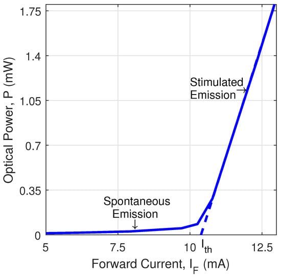
Figure 1.
Steady state Light–Current curve for Laser Diode ADL-65052TL at 15 °C.
The nonlinear function that describes the light–current curve has no explicit dependence on time. Thus, the emitted optical power and the forward current, which represents the output of the system and the control signal , respectively, are defined by:
In our design, the forward current is limited to operating in the stimulated emission zone. Thus, the current is restricted to , where is the maximum forward current defined by the manufacturer. If the system control variable is and the optical power (system output) is , the Equation (1) is rewritten as:
The PI controller (see Figure 2) stabilizes the optical output power around a constant reference, , using a control variable defined in terms of the error signal, , as follows:
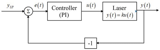
Figure 2.
Block diagram of PI controller.
is the proportional gain, and the integral time. The theoretical design determines a set of rules for and that guarantee convergence to zero or an asymptotically stable behavior of the error signal. If we define the error signal as and we replace it in Equation (4) a more general equation is obtained to describe the output of the system as:
Considering the Leibniz’s rule for derivation under the integral sign and the parameters , ,
as constants, the derivative Equation (5) with respect to time, results in:
The term is rewritten using the chain rule and temperature variation, , as:
If the temperature is stable and the thermal derivative of the slope efficiency, , is bounded, the term described by Equation (7) approaches zero, and the solution of Equation (6) is:
The error signal is defined by:
The solutions proposed in Equations (8) and (9) are valid under the assumption that both equations are solutions of Equation (5). Therefore, replacing the Equation (9) in Equation (5), we find:
The general solution defined in Equation (8) is equated to Equation (10) to obtain the conditions for the solution of simultaneous equations.
Finally, in replacing the condition of Equation (11) in Equations (8) and (9) a particular solution is obtained. Thus,
Equations (12) and (13) show that the error signal is asymptotically stable and that the system output converges asymptotically to if the factor that accompanies the time in the exponential is positive. This factor is known as the characteristic time () of the system and is defined as:
As seen in Equations (12) and (13), the initial condition, , does not directly affect the dynamics of the system. Therefore, the theoretical trajectory of the output is unique and well-characterized. Implying that regardless of the initial conditions of the laser, the response of the system only depends on the control parameters (, , and ) and the slope efficiency (). However, the control variable requires knowing the threshold current for the different operating temperatures. To overcome that issue, the control variable is redefined as . Thus, Equation (3) becomes:
Differentiating the Equation (16) with respect to time and considering a stable temperature (), the terms and can be approximated to zero if the thermal derivatives of those coefficients ( and , respectively) are bounded. Thus, the Equation (6) is obtained, and the solutions proposed in Equations (8) and (9) are also valid.
Finally, the particular solution for a more general control model is rewritten as
3. Numerical Results and Design Restriction
In this section, a numerical analysis is performed to study the behavior of a discrete controller including stability conditions, and numerical limits for the PI control parameters. Initially, we consider the control variable as and the model imposed by the Equation (3). thus, the output of the system i is defined by:
where is the total gain of the system. A numerical solution of Equation (19) can be performed by the Euler method of finite differences, which is equivalent to the iterative model programmed in a real-time controller. The numerical integration is carried out by the Riemann integral method so that the discrete output of the system and the error signal are defined by:
where is the sampling period of the controller, and is the calculation of the accumulated integrated error from 0 to .
A more general numerical solution can be reached by rewriting the time and integral time in terms of an alternative time unit, such as the sampling period (). Hence, the numerical solution is extrapolated to controllers with different sampling periods. The Figure 3a shows the iterative solution of Equations (20) and (21) contrasted with the theoretical solution of Equations (12) and (13), respectively. Both equations show that the particular solution is independent of the initial conditions. Thus, the trajectory of the system output is unique. Additionally, depending on the initial condition, , the system oscillates around the particular solution with an amplitude that depends on the initial numerical error signal, as shown in Figure 3b. Therefore, when the oscillations become imperceptible the trajectories are similar, and the output shows an exponential decay towards .
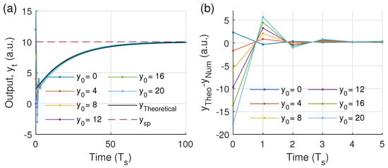
Figure 3.
Comparison between the numerical controller and theoretical system response with operating parameters of = 0.3, = 5, and = 10 for (a) system output. (b) Zoom of differences between the theoretical and numerical output.
However, in [21] is established that oscillations around the output set point appear for high values of . Thus, the oscillations grow exponentially for a certain threshold of the proportional gain making the system unstable (see Figure 4).
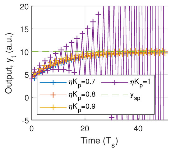
Figure 4.
Numerical analysis of the system output for various total gains and = 4, = 5, and = 10 as fixed system parameters.
According to this, the stability of the system around the theoretical solution is defined by the upper bound of , the integral time (), the numerical method of integration and the effect of the time of sampling, .
The upper limit of was estimated using two iterative integration methods, such as the trapezium rule and the Simpsons’ rule (both methods can be implemented in a real-time controller). Additionally, a characteristic time greater or equal to the sampling period , was chosen.
Equations (22) and (23) describe the numerical integral performed by the controller for the trapezoid method and Simpson’s rule, respectively.
A limit stability condition for the trapezium and the Simpsons’ rule is obtained from the analysis of the numerical solution of the Equations (3) and (4) as is shown in Figure 5 for the three implemented integration methods. On the other hand, the amplitude of output perturbations depends on the initial conditions, ; however, the convergence of this to depends on the integration method and .
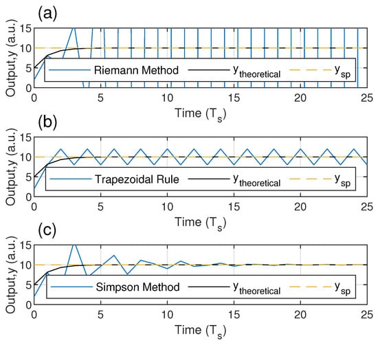
Figure 5.
Convergence analysis of the system output at the stability limit conditions (, and ) for numerical controllers by (a) Riemann’s rule, (b) the trapezoid method and (c) Simpson’s rule and , as fixed parameters of the system.
Additionally, it is established that the limit for the proportional gain is one in controllers working with the trapezoid method or Simpson’s rule. Thus, an interval of that guarantees the asymptotic convergence of the system to is defined by Equation (14) and the numerical limit given by the integration method. If is positive, the proportional gain must meet the following condition to guarantee the convergence of the system to .
If the value of meets the condition of Equation (24) and the characteristic time is greater than , the stability of the system will not be altered. In this way, the upper limit for the condition established in Equation (24) replaced in Equation (14) returns:
Equation (25) is a sufficient condition to guarantee characteristic times greater than the sampling period. However, it is possible to implement integral times that do not meet this condition but meet (defined previously). These integral times require an experimental adjustment of the process or to know a priori the system gain .
4. Experimental Setup
The laser driver circuit design follows the stages of a control system. Therefore, it is divided into a controller, actuator, the system or plant, and a measurement element that provides feedback to the controller with the operating conditions of the system. The different stages of the driver and its electrical diagram are shown in Figure 6 and Figure 7.
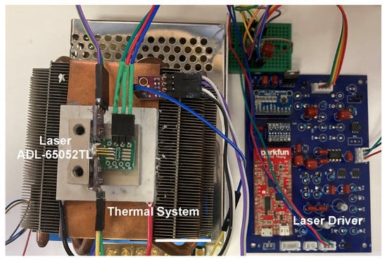
Figure 6.
Experimental setup of the low-cost laser driver.
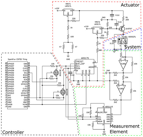
Figure 7.
Electrical schematic of the proposed low-cost laser driver.
The actuator is a current source [24] operating in the active region of a bjt transistor. The current that flows through the laser from the transistor collector is the same as the current on the resistor . Thus, the references 1 () and 2 () potentials define the current on as follows:
The is a fixed voltage source that supplies current to and the laser, while can be adjusted through a digital potentiometer (AD5175) that has a 10-bit resolution (1024 positions) and a nominal resistance of 10 k. As a result, when the potentiometer is set to its maximum resistance (1023 position), reaches its maximum value as well. At this point, the transistor operates in cutoff mode, causing the laser’s supply current to drop to zero. Furthermore, if the potentiometer is set to its minimum (0 positions), which is approximately 0.3 k, reaches its minimum causing the maximum current through and the laser (20 mA).
Nevertheless, the minimum should be higher than the maximum laser operating voltage to prevent the transistor from entering the saturated region. In this case, the transistor operates in the active zone, resulting in a linear relationship between the laser supply current and the position of the digital potentiometer (as shown in Figure 8). Finally, is calculated to ensure that the maximum current over the laser remains below the manufacturer’s current limit.
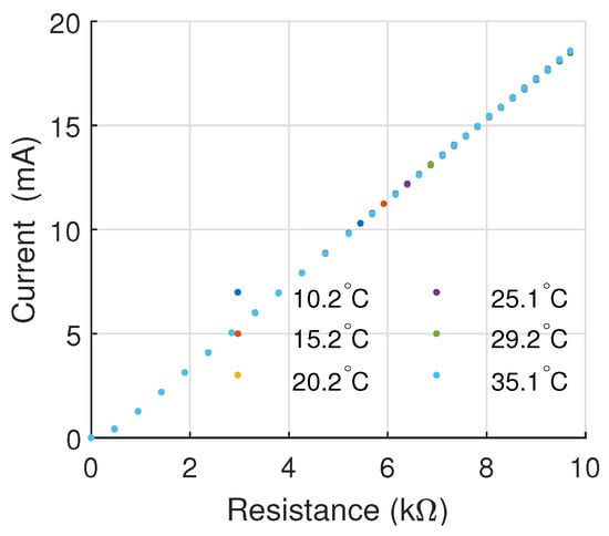
Figure 8.
The linear experimental relationship between the control signal (current supply) and signal actuator (potentiometer positions) at varying operating temperatures.
The measuring element is made up of an internal probe (photodiode) of the laser diode that senses the emitted light power. The photodiode is reverse-biased to obtain a linear response of the current generated by the photodiode and the sensed power. The current from the probing photodiode is converted to a voltage and magnified by a trans-impedance amplifier and an inverting operational amplifier, respectively. The amplified voltage is finally injected into a 16 bits analog–digital converter or ADC (ADS1115) that generates the feedback signal for the controller.
Figure 9 shows the calibration of the feedback signal referenced to the optical power measured directly at the output of the laser using a power meter (Newport, Model 840-C) tuned to a wavelength of 650 nm. In addition, the figure shows that the photodiode of the laser is robust to temperature, and thus the calibration is transversal for the sensed temperature range.
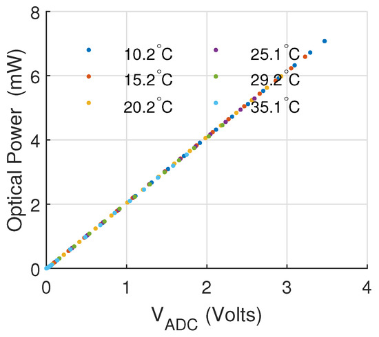
Figure 9.
Calibration of trans-impedance amplifier signal from probing photodiode using emitted optical power measured with a Newport Model 840-C at varying operating temperatures.
The linearity of the actuator and measurement element relationships are shown in Figure 8 and Figure 9. These linear relationships allow the implementation of a controller using the value of the resistance of the potentiometer as a control signal and the voltage of the trans-impedance amplifier as a feedback signal. Finally, a “Sparkfun ESP32 thing” was used as a controller for its low cost and low power consumption.
5. Experimental Results
The proposed IP controller was tested on a laser diode ADL-65052TL under the theoretically established operating conditions and using the trapezoidal integration method. This theoretically guarantees the convergence of the system to with bounded oscillations (see Figure 5b). Experimental tests were conducted at stable temperatures of 15, 20, 25, 30 and 35 °C.
The experimental emission curves (light–current) of the laser were experimentally obtained (see Figure 10) to estimate and . The theoretical system output at the operating temperature was obtained by replacing these terms in Equations (17) and (18). Therefore, a comparison can be made between the experimental output of the system generated by the controller and the theoretical output.
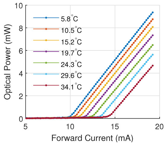
Figure 10.
Experimental laser diode emission curve for a ADL-65052TL at different operating temperatures.
Initially, the response of the system was analyzed with a and an operating temperature of 20.28 °C with a standard deviation of 0.02 °C as shown in Figure 11. There we observed that the theoretical solution did not coincide with the experimental response of the PI controller. This is because the theoretical model of Equation (17) is only valid if the theoretical control signal (Equation (4)) is greater than the threshold current at the operating temperature which is approximately mA.
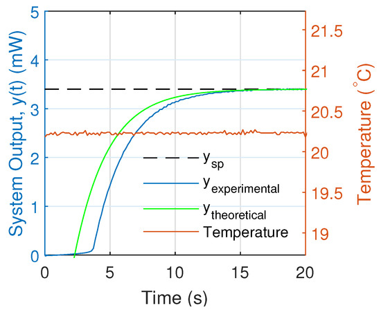
Figure 11.
Comparison of the experimental and theoretical output of the system for a total gain of 0.64 and an integral time of = 1 for an operating temperature of 20 °C.
Figure 12 shows that, when the theoretical control signal is lower than the threshold current, it generates negative theoretical values in the optical power of the laser (see Figure 11).
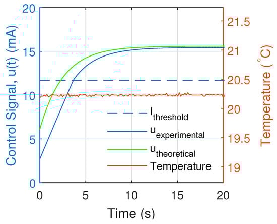
Figure 12.
Comparison of the theoretical and experimental control signal for a total gain of 0.64 and an integral time of = 1 for an operating temperature of 20 °C.
On the other hand, the experimental controller increases the control signal linearly until it exceeds the threshold current. Then, the behavior of the control signal is similar to the theoretical solution, converging the error signal to zero, and the system output to .
The comparison between the theoretical and experimental response of the system requires forcing the controller to operate in the region of stimulated emission of the laser with a control signal greater than the threshold current. This is achieved by modifying the integral in the controller by adding a constant term on the integral so that a new control variable, , is defined as:
The controller of Equation (27) is replaced in the system described by Equation (15). This new differential equation is solved in the way shown previously. Thus, the general solutions of Equations (8) and (9) are applicable to this new control system. The restriction for the particular solution becomes:
Thus, the particular solution for the optical power of the laser is:
Equation (15) indicates that, when the control variable equals the threshold current, the system’s output becomes zero. Therefore, Equation (29) must be zero at . Thus, the value of for this condition is:
The term , according to the Equation (30), is added to the experimental controller, thereby, making the system response similar to the theoretical described in Equation (29) (see Figure 13). Additionally, the experimental and theoretical control signal responses (see Figure 14) are similar when the oscillations produced by the initial conditions of the system disappear.
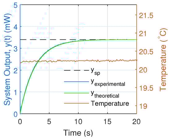
Figure 13.
Theoretical and experimental responses of the system output on the stimulated emission zone for and .
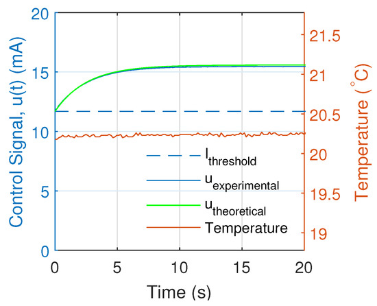
Figure 14.
Theoretical and experimental control signals on the stimulated emission zone for , and .
In addition to forcing the system’s response in the stimulated emission region, Equation (29) provides a theoretical solution for generating a constant output that is centered on . The term is calculated so that the number that accompanies the exponential in Equation (29) is zero, leaving as:
Figure 15 shows the system response under the previous conditions for . There, we observed that the mean value of the output power was centered at with damped oscillations.
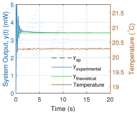
Figure 15.
Experimental response of the system for the constant theoretical output condition with system parameters defined by , and .
A performance test was conducted to simulate how the laser driver works in a space environment of high vacuum at ∼9 Torr (see Figure 16). To achieve this, the laser was operated in a thermal vacuum chamber of NANO-MASTER (NDT-4000). During its operation, the temperature of the chamber was reduced for one hour from 35 °C to −25 °C, which produced a reduction in the temperature on the laser from 30 °C to −10 °C (measured directly on the mount of the laser using a SHT31 temperature sensor) at a rate of ∼0.9 °C/min. During the second hour, the temperature in the chamber was increased from −25 °C to 35 °C to complete the thermal cycle. The driver’s performance is shown in Figure 17. We observed that the maximum and mean variation in the stabilized optical power were 1.3% and 0.4%, respectively.
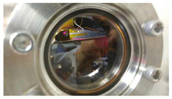
Figure 16.
Image of the laser inside the thermal vacuum chamber (NDT-4000, Nanomaster) during the performance test.
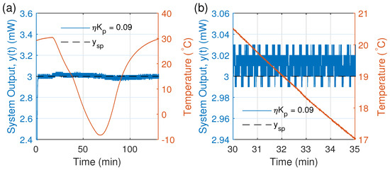
Figure 17.
The laser was evaluated under space conditions. The reached pressure was Torr with the operating temperature varying at a rate of ∼0.9 °C/min. Performance testing was realized by using a thermal vacuum chamber (NDT-4000 from Nanomaster) to emulate the low-Earth orbit conditions. Subplot (a) shows the temporal evolution of the output optical power (blue line) and the temperature (orange line) measured by a SHT31 temperature sensor attached close to the laser. Subplot (b) shows a close-up of the region where the temperature and optical power are dropping from ∼21 °C to ∼17 °C and ∼3 mW ± 2%, respectively.
Finally, the system was forced to operate during a fast change of temperature of ∼9 °C/min as shown in Figure 18b.
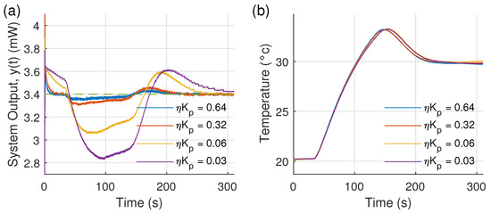
Figure 18.
Robustness of the experimental system output (a) for different from 0.03 to 0.64, s and mW, under thermal disturbances (b).
The instabilities of the system around , or the system error, were dependent on the thermal change rates and value (see Figure 18a). However, the system error began to converge to zero when the thermal change rate became constant or fell to zero. Thus, the designed APC can be used to stabilize the optical output power for a broad temperature range if the control parameters are valid on the temperature range too.
6. Conclusions
A theoretical and experimental study of digital automatic power control (APC) based on a PI controller for a laser diode was performed. This article showed that it was possible to design a digital APC based on a PI controller for semiconductor lasers using the light–current curve obtained either from the one presented in the laser data sheet or experimentally. The control gains () and integral times () that guarantee the convergence of the system to a constant reference were determined in terms of the slope efficiency of the laser.
In Equation (24), an interval for the control gains that guarantees the convergence of the system if the characteristic time of the system is greater than the sampling period or if the integral time complies with Equation (25) was defined.
Nevertheless, the proposed theoretical model does not guarantee the convergence of the system during significant disturbances in the operating temperature that contradict the theoretical assumptions of used in Section 2.
However, the model can guarantee the system stability when the thermal variations are less than ∼1 °C per minute (0.017 °C/s) and if the chosen control gain complies with the condition of Equation (24) in the new operating temperature (see Figure 18).
Furthermore, the analysis demonstrates that, when the thermal variation condition is met, the integral time has no effect on whether or not the system converges. It does, however, allow for the adjustment of the system’s convergence time to the reference . Thereby, the integral time impacts only the system’s characteristic time. Due to the forced behavior of the system that is shown in Figure 3 and described in Equations (12) and (17), it is possible to see that the theoretical convergence time is unique and independent of the initial system conditions (). From the analysis of Equations (12) and (17) (considering ), the value of the convergence time is of five system characteristic times considering a limit of stability for the output system of of . The convergence time can be tuned using the integral time to reach a lower limit of for . Thus, the system response is limited by the sampling period of the controller.
The performance of the designed laser driver compared to other drivers in the literature is shown in Table 1. It is shown that the controller, at stable temperature conditions, achieved slightly better stability (approximately an order of magnitude fewer variations in magnitude) than those reported. Additionally, it can operate during slow thermal variations or slow operating temperature transitions without increasing the instabilities, thus, respecting the other drivers at stable temperature conditions.

Table 1.
A comparison and summary of the main characteristics of the laser controllers cited in the article.
Figure 18 shows the behaviour of the PI controller for more sudden thermal variations. It shows the reduction in robustness of the controller due to the thermal variations, presenting the limit for the proper operability of the controller. The optical power fluctuations are closely related to the controller proportional gain and the thermal speed of change during the operation. Thus, at a low proportional gain and a thermal speed of 0.15 °C/s, the fluctuations reach the 17% of .
Considering the above, it might be necessary to improve the robustness of the driver to thermal fluctuations that might appear during the laser operation in environments where the thermal variations are larger than 0.1 °C/s. A continuous, stable laser can be used for several applications; however, in particular, this type of solution can be useful for nanosatellite applications, where power and volume can be serious constraints. Continuous lasers can be used in propulsion systems, for telescope calibration, and for optical depth instruments (biological experiments in space), to name a few applications. However, the implementation of a modulated current and its effect on the stability of the control will be studied in a future work for other applications such as range estimation (flight formation and space docking), space interferometry, and optical communications applications.
Author Contributions
Conceptualization, J.P. and M.D.; methodology, J.P.; formal analysis, J.P.; investigation, J.P., A.B., J.R., C.P. and M.D.; resources, M.D. and C.P.; writing—review and editing, J.P., M.D. and A.B.; funding acquisition, M.D. and J.P. All authors have read and agreed to the published version of the manuscript.
Funding
This work has been funded by the grants: Agencia Nacional de Investigación y Desarrollo/Subdirección de Capital Humano/DOCTORADO NACIONAL 21212105, QUIMAL 190004, FONDECYT Regular 1221907, FONDECYT Regular 1211695, Programa de Investigación Asociativa (PIA) under Grants ANID ATE 220057 and ANID ATE 220022, Fondo de Equipamiento Científico y Tecnológico (FONDEQUIP) under Grant EQM150138 and ANID BASAL project FB210003. In addition, this material is based upon work supported by the Air Force Office of Scientific Research under award number FA9550-22-1-0299.
Acknowledgments
The authors acknowledge the contributions of referees through their concerns and corrections.
Conflicts of Interest
The authors declare no conflict of interest.
References
- Phipps, C. Laser applications overview: The state of the art and the future trend in the United States. RIKEN REVIEW 2003, 50, 11–19. [Google Scholar]
- Toyoshima, M.; Takayama, Y.; Takahashi, T.; Suzuki, K.; Kimura, S.; Takizawa, K.; Kuri, T.; Klaus, W.; Toyoda, M.; Kunimori, H.; et al. Ground-to-satellite laser communication experiments. IEEE Aerosp. Electron. Syst. Mag. 2008, 23, 10–18. [Google Scholar] [CrossRef]
- Kaushal, H.; Kaddoum, G. Optical Communication in Space: Challenges and Mitigation Techniques. IEEE Commun. Surv. Tutorials 2017, 19, 57–96. [Google Scholar] [CrossRef]
- Li, Q.X.; Yan, S.H.; Wang, E.; Zhang, X.; Zhang, H. High-precision and fast-response laser power stabilization system for cold atom experiments. AIP Adv. 2018, 8, 095221. [Google Scholar] [CrossRef]
- Tricot, F.; Phung, D.H.; Lours, M.; Guérandel, S.; de Clercq, E. Power stabilization of a diode laser with an acousto-optic modulator. Rev. Sci. Instrum. 2018, 89, 113112. [Google Scholar] [CrossRef] [PubMed]
- Phipps, C.; Birkan, M.; Bohn, W.; Eckel, H.A.; Horisawa, H.; Lippert, T.; Michaelis, M.; Rezunkov, Y.; Sasoh, A.; Schall, W.; et al. Review: Laser-Ablation Propulsion. J. Propuls. Power 2010, 26, 609–637. [Google Scholar] [CrossRef]
- Horisawa, H.; Kawakami, M.; Kimura, I. Laser-assisted pulsed plasma thruster for space propulsion applications. Appl. Phys. A 2005, 81, 303–310. [Google Scholar] [CrossRef]
- Blood, P. 1—Principles of semiconductor lasers. In Semiconductor Lasers; Baranov, A., Tournié, E., Eds.; Woodhead Publishing Series in Electronic and Optical Materials; Woodhead Publishing: Cambridge, UK, 2013. [Google Scholar]
- Kondow, M.; Kitatani, T.; Nakahara, K.; Tanaka, T. Temperature dependence of lasing wavelength in a GaInNAs laser diode. IEEE Photonics Technol. Lett. 2000, 12, 777–779. [Google Scholar] [CrossRef]
- Bai, Y.; Bandyopadhyay, N.; Tsao, S.; Selcuk, E.; Slivken, S.; Razeghi, M. Highly temperature insensitive quantum cascade lasers. Appl. Phys. Lett. 2010, 97, 251104. [Google Scholar] [CrossRef]
- Huang, H.; Ni, J.; Wang, H.; Zhang, J.; Gao, R.; Guan, L.; Wang, G. A novel power stability drive system of semiconductor Laser Diode for high-precision measurement. Meas. Control 2019, 52, 462–472. [Google Scholar] [CrossRef]
- Kumar, R.D.; Madhusoothanan, K.N.; Nair, K.R.S.; Ameen, A.P.; Mathew, M.M. A simple cost effective laser driving mechanism for optical communication. In Proceedings of the 2017 IEEE International Conference on Power, Control, Signals and Instrumentation Engineering (ICPCSI), Chennai, India, 21–22 September 2017; pp. 433–435. [Google Scholar]
- Brillant, A. Digital and Analog Fiber Optic Communications for CATV and FTTx Applications; SPIE Press: Bellingham, WA, USA, 2008; Volume 174. [Google Scholar]
- Temel, Ö.D.; Ferhanoğlu, O.; Yelten, M.B. Design of a constant current laser driver for biomedical applications. In Proceedings of the 2021 IEEE 12th Latin America Symposium on Circuits and System (LASCAS), Arequipa, Peru, 21–24 February 2021; pp. 1–4. [Google Scholar]
- Zhao, Y.; Tian, Z.; Feng, X.; Feng, Z.; Zhu, X.; Zhou, Y. High-Precision Semiconductor Laser Current Drive and Temperature Control System Design. Sensors 2022, 22, 9989. [Google Scholar] [CrossRef] [PubMed]
- Ilchev, S.; Andreev, R.; Ilcheva, Z. Ultra-compact laser diode driver for the control of positioning laser units in industrial machinery. IFAC-PapersOnLine 2019, 52, 435–440. [Google Scholar] [CrossRef]
- Ilchev, S.; Otsetova-Dudin, E. Conceptual design and implementation of a microcontroller for the projection of laser and lighting effects in smart environments. In Proceedings of the 23rd International Conference on Computer Systems and Technologies, Ruse, Bulgaria, 17–18 June 2022; pp. 28–32. [Google Scholar]
- Razavi, B. Design of Integrated Circuits for Optical Communications; John Wiley & Sons: Hoboken, NJ, USA, 2012. [Google Scholar]
- Zivojinovic, P.; Lescure, M.; Tap-Beteille, H. Design and stability analysis of a CMOS feedback laser driver. IEEE Trans. Instrum. Meas. 2004, 53, 102–108. [Google Scholar] [CrossRef]
- Huan, W.; Zhigong, W.; Jian, X.; Yin, L.; Peng, M.; Siyong, Y.; Wei, L. A fast automatic power control circuit for a small form-factor pluggable laser diode drive. J. Semicond. 2010, 31, 065014. [Google Scholar] [CrossRef]
- Åström, K.; Hägglund, T. PID Controllers: Theory, Design, and Tuning; ISA—The Instrumentation, Systems and Automation Society: Research Triangle Park, NC, USA, 1995. [Google Scholar]
- Silva, G.J.; Datta, A.; Bhattacharyya, S.P. PID Controllers for Time-Delay Systems; Springer: New York, NY, USA; Berlin/Heidelberg, Germany, 2005; Volume 43. [Google Scholar]
- Paschotta, R. Basic Principles of Lasers. In Field Guide to Laser Pulse Generation; SPIE Press Bellingham: Bellingham, WA, USA, 2008; Volume 14, pp. 1–15. [Google Scholar]
- Horowitz, P.; Hill, W.; Robinson, I. The Art of Electronics; Cambridge University Press: Cambridge, UK, 1989. [Google Scholar]


Disclaimer/Publisher’s Note: The statements, opinions and data contained in all publications are solely those of the individual author(s) and contributor(s) and not of MDPI and/or the editor(s). MDPI and/or the editor(s) disclaim responsibility for any injury to people or property resulting from any ideas, methods, instructions or products referred to in the content. |
© 2023 by the authors. Licensee MDPI, Basel, Switzerland. This article is an open access article distributed under the terms and conditions of the Creative Commons Attribution (CC BY) license (https://creativecommons.org/licenses/by/4.0/).