Article

A Study on Using Location-Information-Based Flow Field Reconstruction to Model the Characteristics of a Discharging Valve in a Hydrodynamic Retarder

1
National Key Laboratory of Vehicular Transmission, Beijing Institute of Technology, Beijing 100081, China
2
Beijing Institute of Technology Chongqing Innovation Center, Chongqing 401120, China
3
Institute of Advanced Technology, Beijing Institute of Technology, Jinan 250307, China
*
Author to whom correspondence should be addressed.
Machines 2023, 11(4), 460; https://doi.org/10.3390/machines11040460
Submission received: 16 February 2023 / Revised: 31 March 2023 / Accepted: 4 April 2023 / Published: 6 April 2023
(This article belongs to the Section Machine Design and Theory)

Abstract

:
In modeling the characteristics of a discharging valve in a hydrodynamic retarder, it is commonly required to determine the value of the flow area to calculate the force on the spool. However, the flow area often relies heavily on empirical or simulation data, which leads to increased uncertainty and computational cost, especially with the variation in the spool displacement. To overcome these shortcomings, Res-SE-U-Nets (networks that combine residual connections, squeeze-and-excitation blocks, and U-Net) are used to reconstruct the velocity field, and they have shown exceptional performance in image-to-image mapping tasks. The dataset of computational fluid dynamics (CFD) results for the velocity field is collected and verified using particle image velocimetry (PIV). The results show that Res-SE-U-Nets can capture the location information of the flow field using a training set of only 120 data points. By utilizing location information in velocity field reconstruction, the flow area can be directly obtained under different spool displacements and pressures to calculate the spool force. The valve characteristics calculated with this method show an error of less than 2% when compared with CFD results, which confirms the validity and effectiveness of this method. The proposed method, which utilizes location information extracted from flow field prediction results, is capable of calculating valve characteristics. This approach also demonstrates the feasibility of using Res-SE-U-Nets for flow field reconstruction.

1. Introduction

A hydrodynamic retarder is a kind of auxiliary braking that is widely used on heavy-duty vehicles to avoid brake overheating and failure caused by frequent braking [1]. For hydrodynamic retarders, the spool displacement of the discharging valve can effectively adjust the oil filling rate in the wheel cavity, changing the braking torque, which keeps the speed constant when the vehicle is continuously braking down a long slope. In the design of hydraulic components, it is crucial to study the influence of different design parameters on the flow characteristics of the internal flow field [2]. Three-dimensional simulation of the flow field techniques can accurately predict flow fields of different design parameters, revealing the influence of different parameters on the flow characteristics [3]. However, solving such complex problems using traditional simulation methods requires a high-quality mesh and considerable amount of time, resulting in a high cost of simulation calculation [4]. Instead, the data-based flow field construction model enables engineers to quickly overview the flow characteristics of a flow field [5,6].
To establish the mapping relationship between design parameters and flow field results, a combination of computational fluid dynamics (CFD) and response surface model (RSM) can be used, which is widely employed in optimization problems [7]. Zhang et al. [8] established a surrogate model for pressure relief valves using RSM. In this work, a sensitivity analysis was performed after CFD to establish a mapping relationship between the shape and blowdown capacity of the pressure relief valve. Yang et al. [9] established the relationship between four variables and three optimization targets in hydrodynamic retarders and carried out a multiobjective optimization design. In this work, CFD was used to obtain the optimized retarder flow field to analyze the influence of design parameters on the vortex field distribution. From the above research, it can be found that RSM can only establish a mapping relationship on scalar values, which lacks the vector information of the flow field compared with CFD. Artificial neural networks have more power to establish a nonlinear relationship between input and output [10]. However, similar scalar-based surrogate models have the same shortcomings. It is difficult to obtain accurate or inductive results in the simulation analysis, where location information is more important [11]. To reduce the flow field data and reconstruct the unknown flow field, the proper orthogonal decomposition (POD) method can decompose the flow field data into multiple modes, sort the primary and secondary ordering, and use the dominant mode to describe the original flow field accurately [12]. Kong et al. [13] established the extraction of the main features of the flow field using POD. The results show that POD can effectively reconstruct the pressure field and velocity field. Wang et al. [14] used the POD method to reconstruct the three-dimensional flow in a complex flow channel, analyzing the physical meaning of reconstructed flow field in different modes. The principle of POD is to project the control equations onto the fundamental modes, not to establish the relationship between different positions in the physical area [15]. While the POD method is a widely used technique for flow reconstruction, it requires optimization for specific flow structures, and changes in flow structure or channel shape may require reanalysis and rebuilding. In contrast, a deep-learning-based method provides an alternative to the conventional POD method for flow field reconstruction. By utilizing a single model to predict the flow field, the deep-learning-based method effectively addresses this limitation, regardless of the flow structure.
The deep learning approach to flow field reconstruction, utilizing datasets constructed from CFD results and allows for quick prediction of the flow field in response to changes in channel geometry, thereby reducing computational costs associated with CFD [16]. Ribeiro et al. [17] obtained the velocity field and pressure field using convolutional neural network (CNN). The results show that the method is able to learn the complete solutions of the Navier–Stokes equations. Obiols-Sales et al. [18] proposed a coupling framework for CFD and deep learning which uses CNN to calculate the rotor velocity field, pressure field, and vortex viscosity. In this study, the proposed method is able to obtain the flow field under different operating conditions and rotor shapes. Sekar et al. [19] used deep learning to express the geometric shape nonparametrically and reversely design the airfoil. The results show that the airfoil shape can be obtained according to the pressure coefficient distribution using CNN. Thuerey et al. [20] predicted the pressure field and velocity field of the rotor based on the U-Net network and researched the allocation of datasets and weights. The results show the possibility of using deep learning to predict the flow field. Deep learning methods use GPUs to obtain CFD results, which can reduce the prediction time through parallel computation [21]. Flow field reconstruction technology based on deep learning methods effectively extracts flow field data. However, the requirements for model scale are relatively high. It is necessary to reasonably construct the model, set various hyperparameters, and select appropriate input features and extraction methods. Among various deep learning architectures, Res-SE-U-Nets have emerged as a promising approach that combines the strengths of residual connections, squeeze-and-excitation blocks, and U-Nets to enable effective feature extraction. In a recent study, Res-SE-U-Nets were shown to exhibit exceptional performance in image-to-image mapping tasks [22,23]. The above studies primarily focus on developing surrogate models using deep learning methods, with less emphasis on the practical utilization of prediction results.
In this study, based on CFD results, a velocity field reconstruction model of the discharging valve was developed using Res-SE-U-Nets. First, the velocity field of the discharge valve was obtained under different spool displacements and pressure differences with CFD. Second, the reliability of the CFD results was verified by particle image velocimetry (PIV). Then, Res-SE-U-Nets was trained with the simulation-driven small dataset. Finally, the flow area is extracted in the reconstructed velocity field and used to calculate the steady-state flow force. This means that the uncertainty and inaccuracy caused by the empirical formula calculations are avoided.

2. Methodology

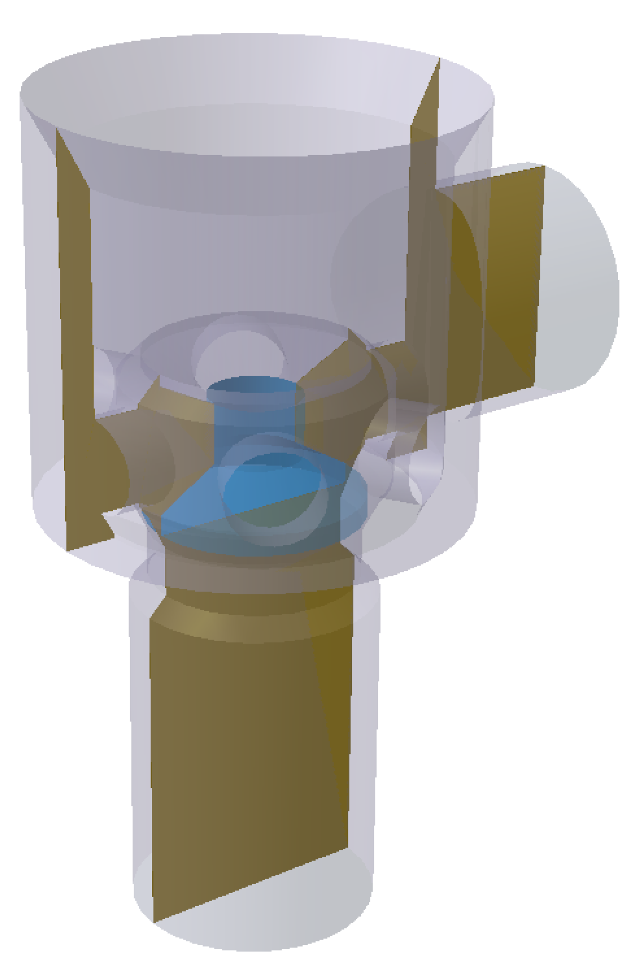
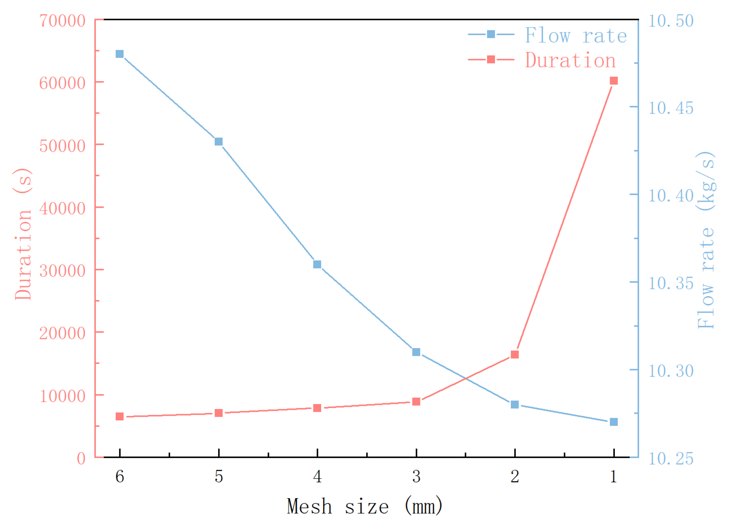
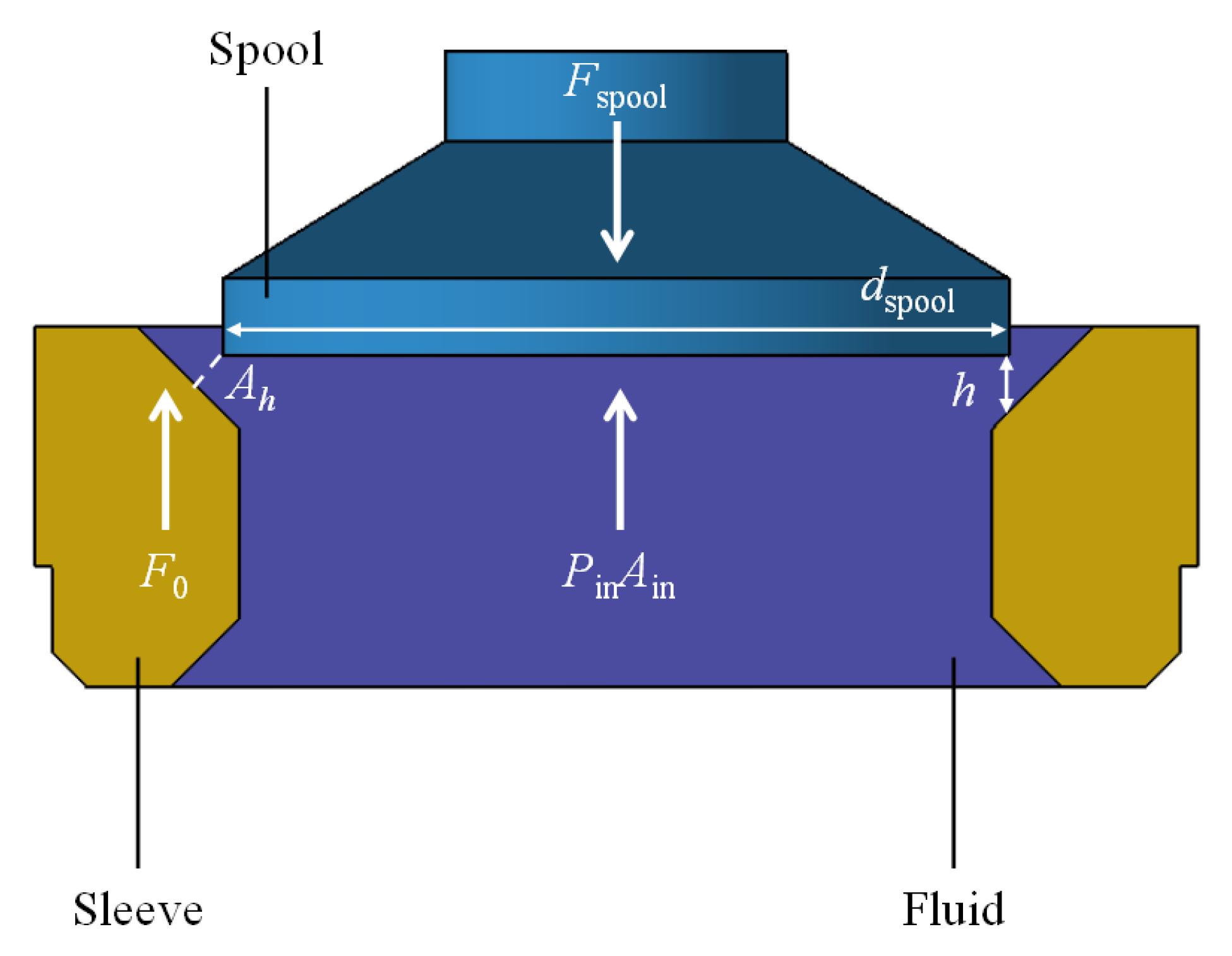
2.1. Discharging Valve Simulation

The internal flow field of the hydrodynamic retarder discharging valve are affected by the spool displacement [24]. To obtain the velocity field of the valve under different spool displacements and pressure differences, a steady-state flow simulation by CFD was conducted first, as shown in Figure 1.
After the geometry cleanup of the discharging valve simulation model, a hexahedral mesh was used for meshing. The size of the mesh can have a significant impact on the numerical solution [25]. Due to the limited solving power of computers, it is necessary to use an appropriate grid size that allows for accuracy, while avoiding high computational costs. The global mesh size and corresponding flow rate and time consumption are shown in Figure 2. In our study, we determined the final mesh size to be 2 mm, resulting in approximately 660,000 meshes. The robust k ω S S T model was used to capture the flow characteristics of the flow field [26]. As required by the y + criterion, the total thickness of the boundary layer is 1 mm, the mesh growth rate is 1.2, and there are 5 boundary layers in total.
According to the material properties of oil in tests, the density of the oil is 860 kg/m 3 , and the dynamic viscosity is 0.028 Pa·s. Boundary conditions were set according to the operating conditions of the valve. The inlet boundary condition is set as a stagnant inlet, the outlet boundary condition is set as a pressure outlet, and the rest of the walls are set as no-slip walls. The oil is assumed to be an incompressible viscous fluid, and the velocity of the fluid near the nonslip wall is the same as the given velocity value of the wall.
In this paper, a numerical simulation of the discharging valve was performed with FLUENT. When the solution converges, the velocity field of the valve can be derived. To verify the accuracy of the CFD results, an experimental test platform was built using PIV technology to observe the velocity field. PIV is a noncontact flow field measurement method. Since the 1980s, it has been mainly used in flow visualization research and has been widely used in valve research [27]. In this study, the experimental system shown in Figure 3 is constructed, which mainly includes optical test components, a laser section generation system, and an image acquisition system. An MGL-N-532-5W all-solid-state laser and a high-speed camera model SpeedSense VEO 410 are used. Silver glass microbeads are used as tracer particles, matched with No. 110 nonfluorescent industrial white oil to ensure the visibility of the tracer particles inside the oil.
According to the CFD results, the velocity field distribution in the X direction and the Y direction of the discharge valve section is obtained. The simulation results are compared with the PIV test results in this area, as shown in Figure 4 and Figure 5. In image processing, the comparison between images is essentially a matrix operation. Consequently, the PIV test results and CFD calculation results are converted into numerical matrices, and matrices A m n and B m n are constructed for v ¯ ( x , y ) . Matrix correlation analysis is used to compare the correlation between CFD and PIV images. The correlation coefficient r between matrices is defined as follows [28]:
r = m n ( A m n A ¯ ) ( B m n B ¯ ) ( m n ( A m n A ¯ ) 2 ) ( m n ( B m n B ¯ ) 2 )
where A m n is the value of PIV image matrix, B m n is the value of the CFD simulation image matrix, and A ¯ and B ¯ are the mean values of the PIV and CFD image matrices, respectively.
Based on the correlation analysis, as shown in Table 1, strong correlations were found in both X and Y directions at low flow velocities, while a medium correlation was observed at high flow velocities [29].
In the X direction, no obvious velocity missing areas were detected, as shown in Figure 4. The oil velocity field distribution exhibited similar characteristics, with high-speed regions gradually concentrating at the cone angle of the spool as velocity increased. However, the PIV test results show a slightly higher overall velocity amplitude in the X direction compared with CFD simulation results. This difference is attributed to limitations in test site and equipment, which led to actual PIV test results being larger than the expected settings.
In contrast, the Y-direction comparison revealed a missing velocity region in the PIV image, as shown in Figure 5. Both simulation and test results show a significant increase in overall velocity amplitude as the flow rate was increased, particularly at the spool to the right wall, where high-speed flow regions were observed. However, missing particles themselves were more susceptible to the influence of gravity, leading to larger differences between velocity distribution in the Y direction and CFD calculation results. As a result, the integrated correlation coefficient and flow field distribution confirmed the accuracy of the numerical calculation results.

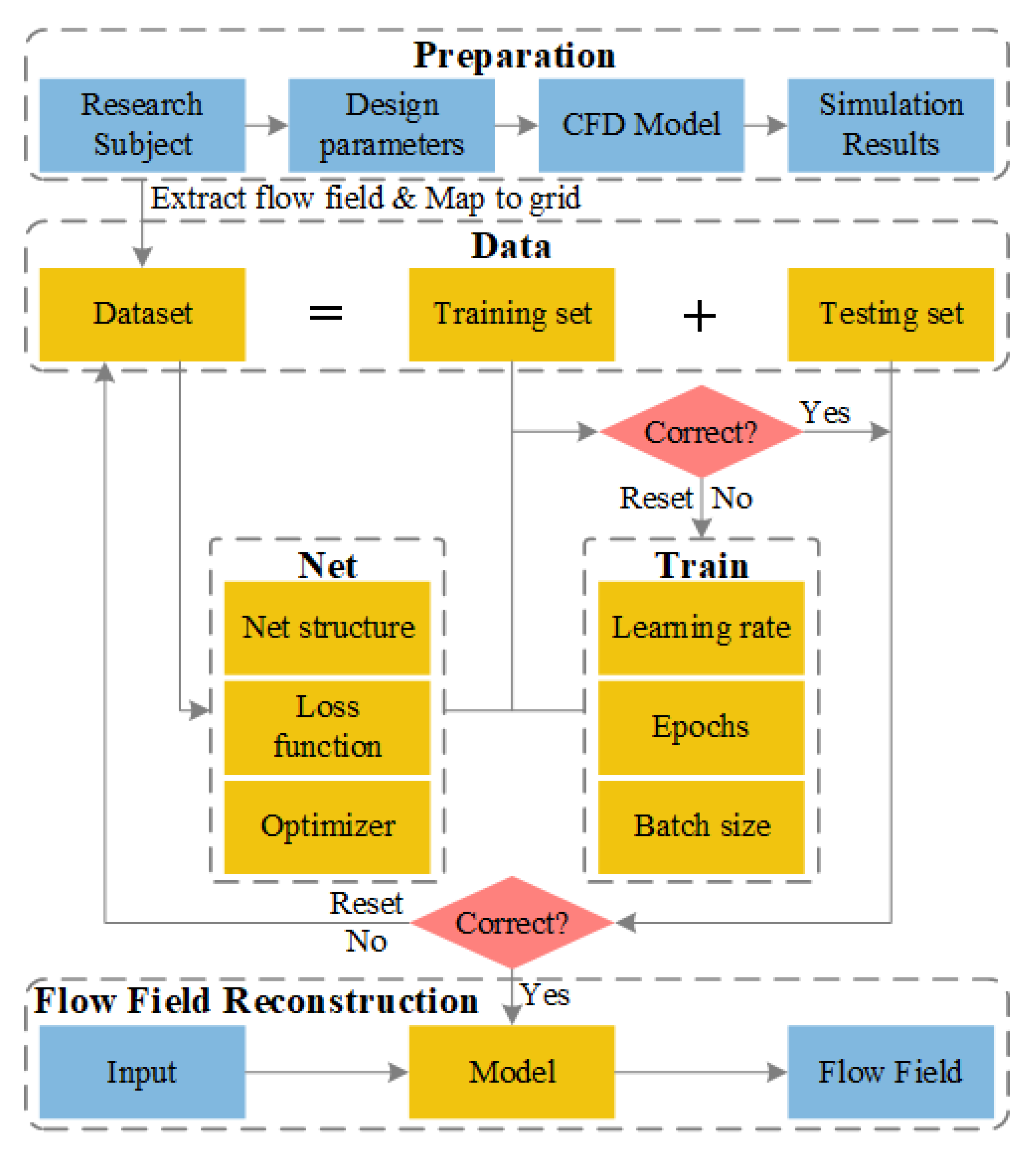
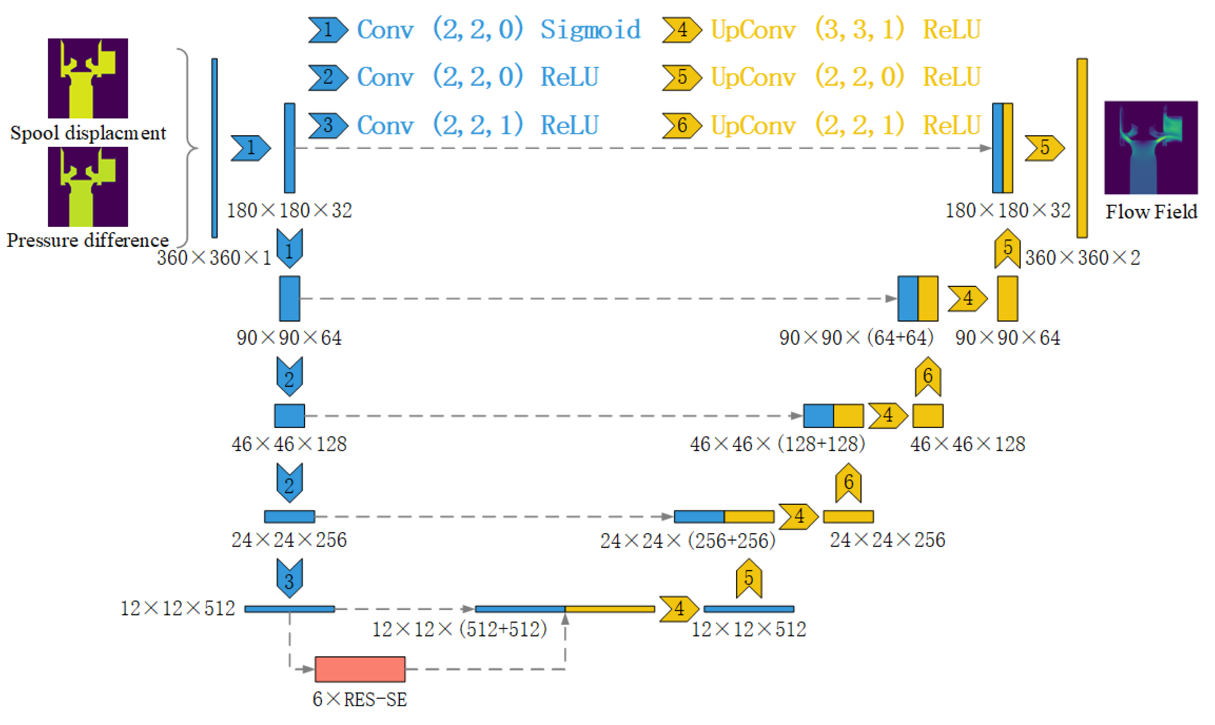
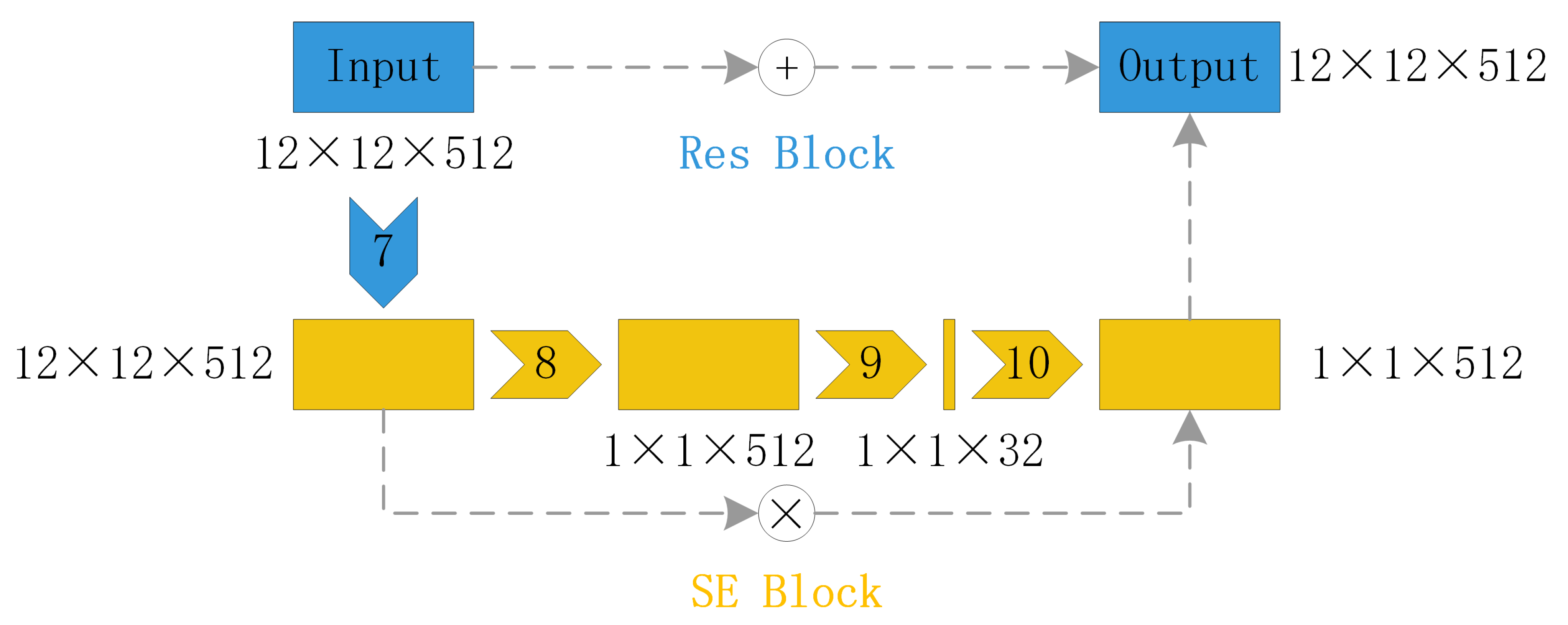
2.2. Flow Field Reconstruction Using Deep Learning

The deep learning flow field reconstruction model can extract geometric features and rules from input data to obtain the same flow field as CFD [30]. This paper utilizes CFD simulation results as a dataset to train the deep learning model and reconstruct the flow field, as shown in Figure 6. The trained model is verified with a test set, and the flow field prediction model is obtained if it passes verification without underfitting or overfitting. Otherwise, the training and testing process needs to be repeated with new parameters and dataset.
The deep learning model used in this paper is based on the U-NET structure, which is widely used in semantic segmentation [31]. To further enhance the prediction capability and location information extraction ability of U-Nets, the Res-SE module consists of a residual network, and an attention mechanism is added before the upsampling of U-Nets [32], which leads to Res-SE-U-Nets, as shown in Figure 7. The specific parameters and related activation functions of each layer are shown in Table 2. The RES module can deepen the influence of shallow networks and avoid accuracy decay through residual connections. In the SE module, the global pooling layer is used to compress each two-dimensional channel into a real number, and then two fully connected layers are used to establish the correlation between channels and obtain weights. The resulting normalized weights are applied to each channel. The SE module is combined with the RES module, which means combining the attention mechanism with the residual network, as shown in Figure 8.
According to the simulation model, the input variables are discretized into 360 × 360 pixels, and each input comprises two image channels. The size and the number of channels mainly depend on the grid size and the number of variables in the CFD [33]. In downsampling, the image size is gradually reduced from 360 × 360 to 12 × 12, and the number of channels is increased from 2 to 512. The purpose is to fully extract the location information under different variables in the input image. The images are then processed by 6 serial Res-SE blocks and imported for the upsampling, where the images of size 12 × 12 are increased to feature images sized 360 × 360 by a series of deconvolution layers. After the processes of downsampling, RES-SE blocks, and upsampling, the input images are increased into an output image of 360 × 360 × 1, which corresponds to the prediction result in the simulation model. In this process, the images in the downsampling will be added to the upsampling through the residual connection to enhance the location information extraction ability of the model.
The Adam optimization algorithm is used as the optimizer [34], and the activation function uses two functions: sigmoid and ReLU. The mean square error (MSE) loss is applied to calculate the similarity between the calculated model and the expected output, which is widely used to evaluate artificial intelligence models, and the MSE loss is defined as follows [35,36]:
M S E = 1 n n i = 1 ( y ^ i y i ) 2
where n is the total output, y ^ i is the expected value of the i-th element of the output vector, and y i is the calculated value of the i-th element of the output vector.

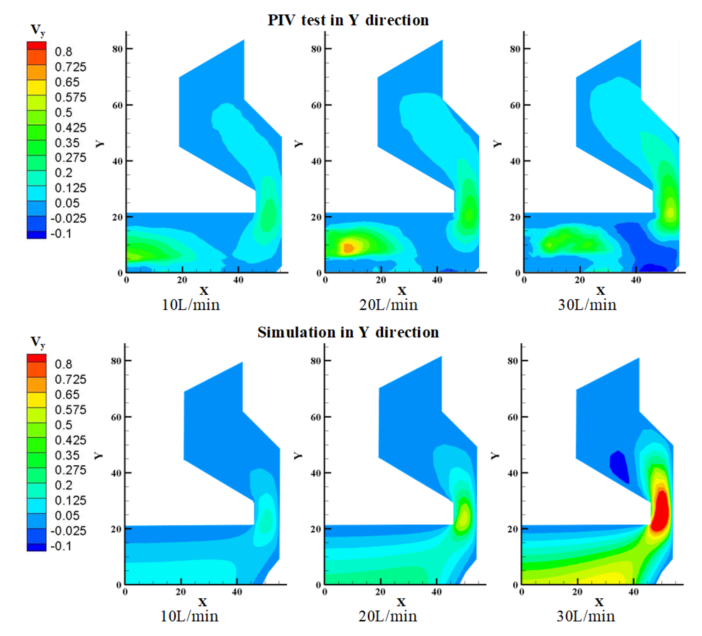
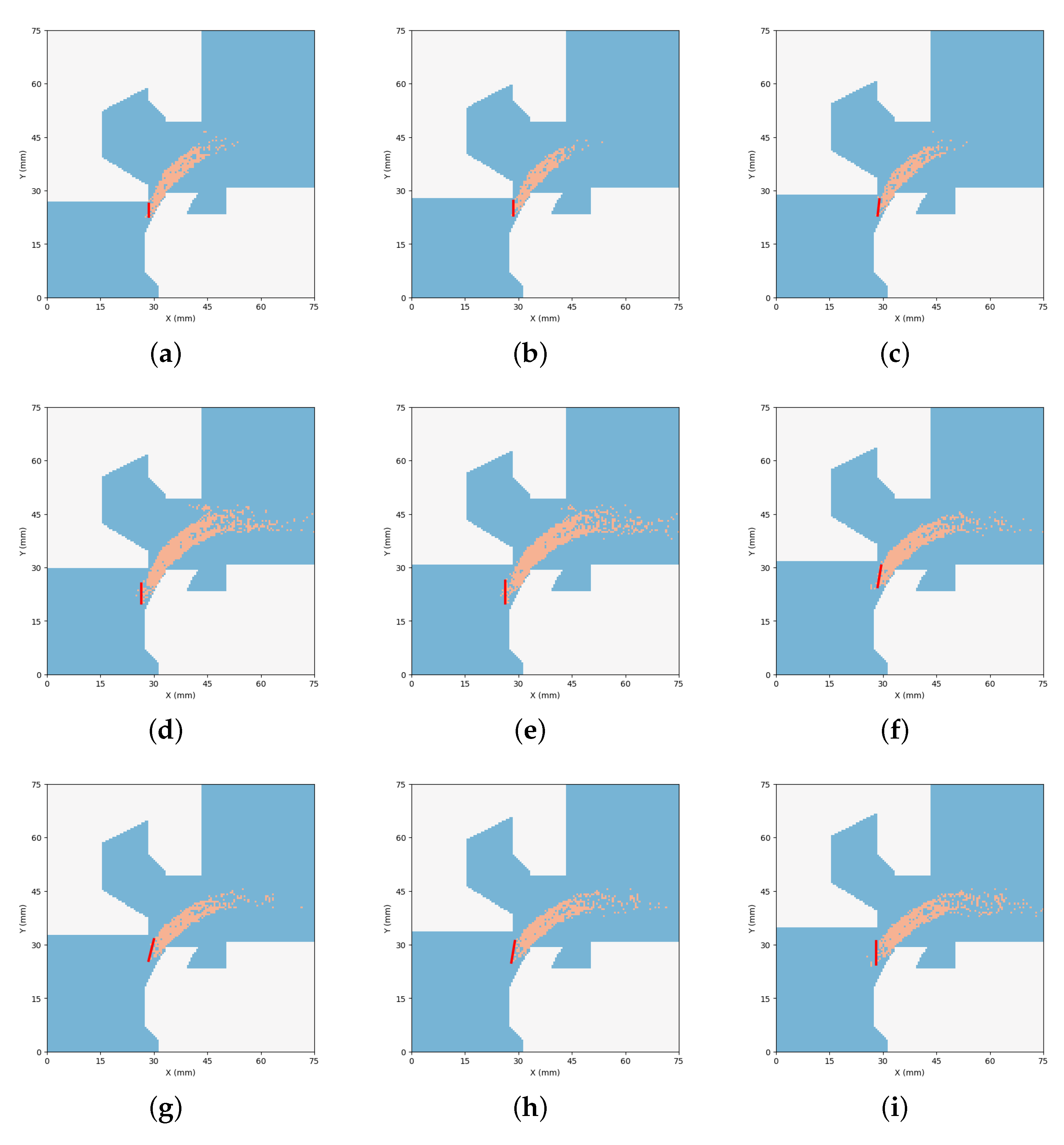
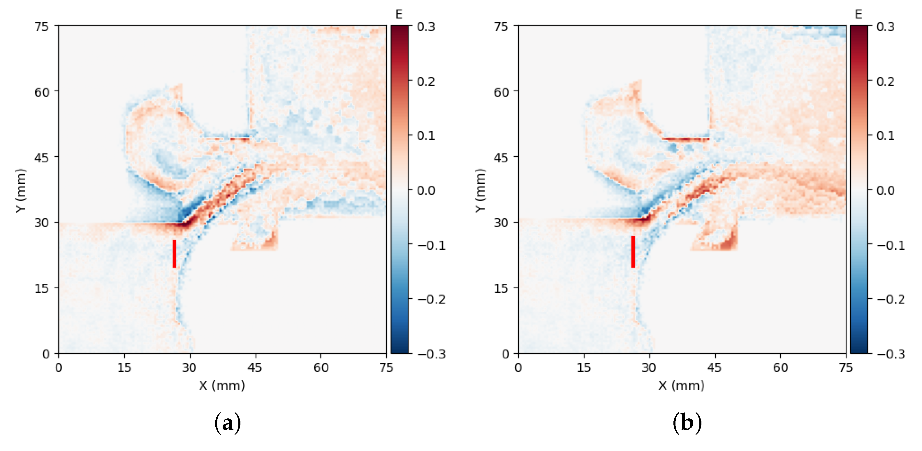
3. Velocity Field Reconstruction

3.1. Simulation-Driven Dataset

According to the CFD results of the discharge valve, the velocity field under different spool displacements h and pressure differences Δ p is obtained. The changes in different spool displacements with position information lead to changes in the internal flow path structure, thereby changing the flow field of the discharge valve. The above two variables are selected as input, and the velocity field of the discharge valve section is used as output to construct the dataset. The value range of the spool displacement h is 1 mm to 15 mm, and the value interval is 1 mm. The value range of the pressure difference Δ p is 1 bar to 9 bar, and the value interval is 1 bar. The CFD results of different design parameters are obtained, and the datasets contain 135 samples, which are shuffled and then divided into a training set and a test set according to the test ratio of 8:1.
To verify the feasibility of small datasets in simulation-driven deep learning flow field reconstruction, the datasets constructed in this paper contain only 135 samples. For simulation-driven datasets, unlike the classification problem, there is a corresponding relationship with physical meaning between the input and output. For example, in the flow field of the discharge valve in this study, the output reflects the flow velocity, and there is a physical law between pressure and velocity [37]. In classification problems, the result of the output vector usually abstractly refers to a certain category of subjects. In addition, during the training process, the dataset comes from the CFD results, which are obtained under the constraints of various boundary conditions and reflect the inherent characteristics of the fluid in the steady state. Therefore, the samples contain less noise, which reduces the training difficulty of the model. The above factors are conducive to establishing the mapping relationship between input and output in deep learning training, which can effectively reduce the size of the dataset [38].
Another purpose of using CFD results to establish the datasets is to show that the established model can effectively extract location information in the flow field without relying on big data. To illustrate the importance of location information in the flow field, Figure 9 shows the influence of different spool displacements on the velocity field when the pressure difference between the inlet and outlet is 9 bar. As the spool displacement increases, the direction of the oil velocity at the orifice changes. This will lead to a change in the flow area, which shows that location information in the flow field is necessary. The pressure–flow characteristics of valves are crucial in describing their ability to control fluids, and related simulations and experiments reflect the valve’s performance in relation to variations in pressure–flow characteristics [39,40]. Figure 10 displays the velocity field of the discharging valve with varying inlet and outlet pressure differences, observed at an 8 mm spool displacement. As the pressure difference increases, the flow rate within the discharging valve also increases.

3.2. Results Analysis

To evaluate the flow field reconstruction ability of Res-SE-U-Net, the trained model is applied to predict the velocity field of the discharge valve, and the test set is used for verification. To test the ability of the prediction model to extract flow field location information, pixel-wise error (PWE) is applied to evaluate the difference between the simulated flow field and the predicted flow field. Figure 11 and Figure 12 show the simulated flow field, reconstructed flow field, and pixel-to-pixel error maps of the training set and test set.
The reconstructed flow field is almost the same as the simulated flow field, the PWE value is small, and the large error mainly occurs near the wall, where the velocity gradient changes greatly, as shown in Figure 11. The flow field reconstruction model maps the data as a 360 × 360 pixel image, which leads to the neglect of velocity gradient variation near the wall. This is the main reason for the large error observed in the near-wall region. However, it should be noted that the location information can still be obtained accurately, since the reconstructed flow field is almost the same as the simulated flow field in other regions.
The PWE of the test set is slightly larger than that of the training set, and the main distribution area of the large error is also concentrated near the wall. The error value has little influence on the overall flow characteristics, and the error is within an acceptable range, as shown in Figure 12. The error of the traditional surrogate model such as RSM can only reflect the magnitude of the value, but the error of the model in this paper can reflect the location information of the error, providing more information to analyze the original source of the error.
The above analysis shows that Res-SE-U-Nets flow field reconstruction model can effectively extract location information, predict unknown flow fields, and realize flow field visualization. Compared with the surrogate model that only predicts scalar data, the flow field reconstruction method based on deep learning provides more information for flow field research.

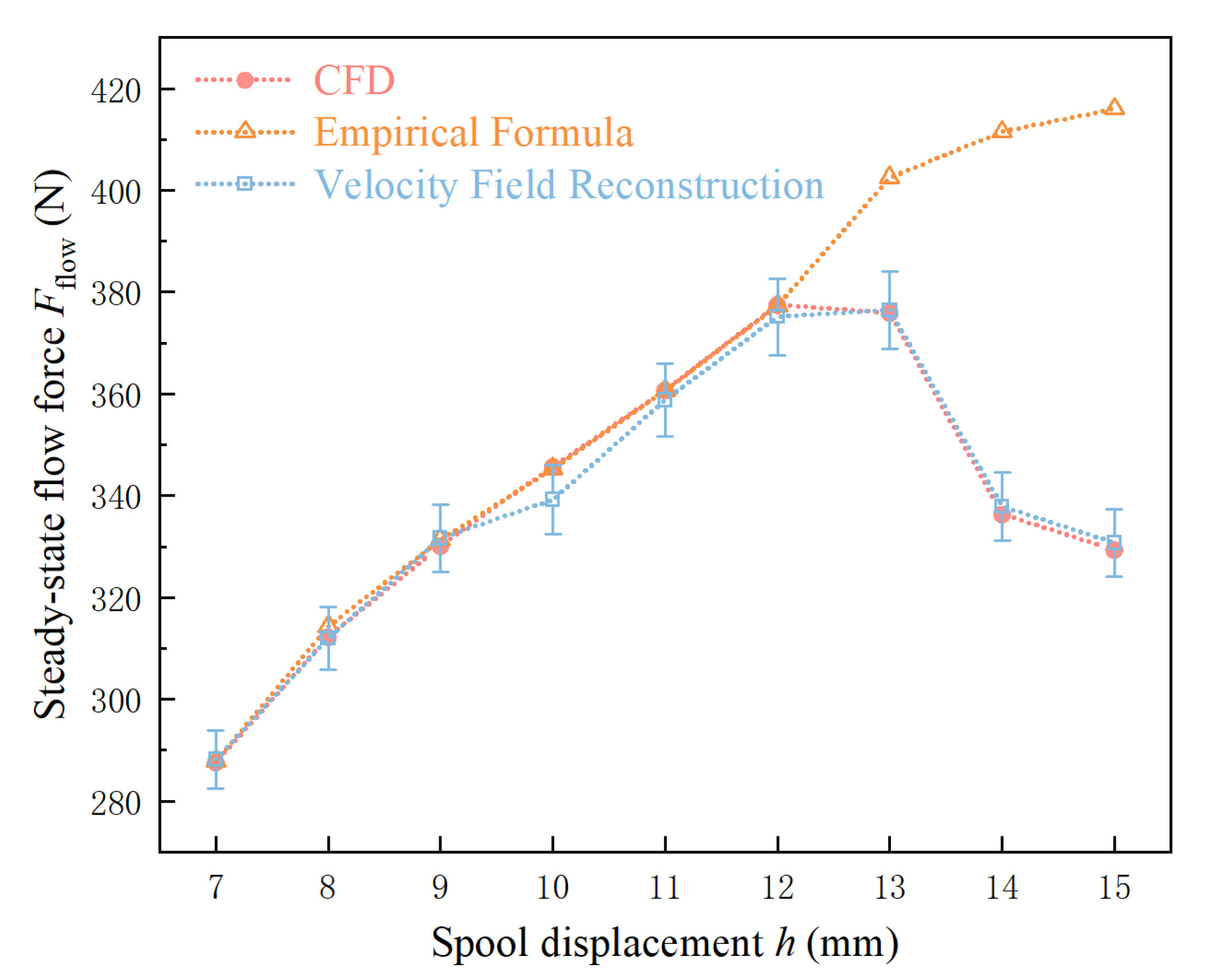
4. Steady-State Flow Force Calculation

In the study of the discharging valve, the flow force has a great influence on the balance and opening characteristics of the spool [41]. Theoretically, the force of the oil on the spool depends on the inlet pressure and the area of the spool. However, the oil velocity at the orifice changes abruptly in direction and magnitude, which in turn affects the pressure distribution at the bottom of the spool. The actual force on the spool is less than the theoretical force because of the presence of flow force. The flow force is divided into the steady-state flow force and transient flow force. The transient flow force is too small to be ignored, so the steady-state flow force is mainly considered when analyzing the force on the spool. Figure 13 shows the structure of the discharging valve, which is mainly composed of a spool and sleeve.
Considering the force on the spool and using Newton’s third law, the steady-state flow force F flow can be expressed as [42]
F flow = P in A in + F 0 F spool
where P in is the inlet oil pressure of the valve, A in is the flow area of valve, F 0 is the force exerted by the sleeve, and F spool is the force of the oil acting on the spool.
Applying the momentum theorem, the steady-state flow force can be expressed as [43]
F flow = ρ q ( v 2 cos α v 1 )
where ρ is the oil density, q is the flow rate of the valve, α is the jet angle, v 2 is the oil flow rate at the valve outlet, and v 1 is the oil flow rate at the valve inlet.
According to the empirical formula [44], the above equation can be simplified. The jet angle α can be replaced by the semicone angle of the sleeve. The inlet flow rate v 1 can be ignored, since it is much smaller than the outlet flow rate v 2 . The flow area A in is simplified as the vertical surface at the nearest position from the sleeve to the spool. According to the flow formula of the valve, the steady-state flow force can finally be expressed as
F flow = 2 C d 2 A h cos θ Δ P
A h = π h sin α ( d spool + 1 2 h sin 2 α )
where C d is the flow coefficient and is taken as a constant value of 0.7, according to the Reynolds number > 1000 in this study [45], A h is the flow area when the spool displacement is h, θ is the semicone angle of the sleeve, Δ P is the pressure difference between the inlet and outlet of the valve, h is the spool displacement, and d spool is the diameter of the spool.
In the flow field inside the discharge valve, the velocity and pressure around the spool will change sharply. It is difficult to accurately describe the distribution of velocity or pressure with empirical formulas. In the traditional method, to accurately calculate the steady-state flow force, it is necessary to establish a CFD model, which involves a large calculation cost. By using Res-SE-U-Nets, the velocity field can be quickly reconstructed, and the velocity distribution around the spool, as well as the flow field including location information such as the jet angle and flow area, can be obtained. Therefore, the calculation problem of the steady-state flow force is effectively solved, and the calculation accuracy is guaranteed, while the flow field is reconstructed rapidly. When using a fluid field for steady-state flow calculation, instead of simply using numerical values for fitting, the flow area is obtained directly from the image. Figure 14 shows the postprocessing results of the fluid field reconstruction with a pressure difference of 9 bar under different spool displacements. The points with a large velocity gradient in the velocity field are extracted, which are approximately distributed on the line with the shortest distance between the spool and the sleeve. The boundary line formed by the extracted points can be regarded as the flow area of the discharge valve, which can be used to calculate the steady-state flow force.
The size and direction of the flow area change with increasing spool displacement, which is not consistent with the assumptions of the empirical formula. Therefore, the adoption of the empirical formula for the flow area will lead to errors. The magnitude of the steady-state flow force is calculated according to the flow area by the flow field reconstruction and compared with the calculated value of the empirical formula and the CFD, as shown in Figure 15. When the spool displacement is greater than 12 mm, the bottom of the spool is higher than the sleeve. In this case, the empirical formula is no longer applicable, so the calculation results are distorted. However, the flow field reconstruction results contain location information, so the flow area can be extracted according to the physical meaning. The calculation result is not affected by the change in the flow channel structure. Although the error of h = 10 mm was slightly larger, the final error in the flow force calculation was less than 2%.
Upon observing the curve calculated based on the field reconstruction, a larger error was found at the spool displacement of 10 mm. Upon comparing the error plots for h = 10 mm and h = 11 mm, it was discovered that the error near the 10 mm overflow section was greater than that of 11 mm, as illustrated in Figure 16. The error diagram for h = 10 mm indicated a larger error in the region of the orifice, where larger points of velocity gradient are concentrated. This error affected the extraction of the flow area. On the other hand, the error of h = 11 mm showed less error near the orifice and accurately reflected the jet angle. This analysis reflects the advantage of the proposed method in this paper. The method effectively analyzes errors using location information in the prediction results and clarifies their cause. Therefore, the method proposed in this paper can effectively extract location information in the flow field and calculate the steady-state flow force.

5. Discussion

In this study, a deep learning method was proposed for the reconstruction of velocity fields in the discharging valve of a hydrodynamic retarder. The purpose of this method is to overcome the shortcomings of relying heavily on empirical or simulation data to determine the flow area, which leads to increased uncertainty and computational cost, especially with the variation of the spool displacements.
Firstly, the accuracy of simulation results was validated by comparing them with experimental data obtained using PIV tests. The results show a strong correlation in the X direction (0.60–0.73) and a strong or medium correlation in the Y direction (0.42–0.57). The agreement between the simulated velocity field distribution and that obtained by Kong et al. [13] provides further confirmation of the accuracy of our simulation analysis. Additionally, the PIV test results provide a visual observation of the velocity field, which deepened the understanding of the internal flow field distribution and flow structure.
Secondly, Res-SE-U-Nets were utilized to predict the velocity field of the discharging valve. The pixel-to-pixel error results shown in Figure 11 and Figure 12 demonstrated that the model could produce results consistent with simulation results. Res-SE-U-Nets have been used in simulation surrogate model studies in multiple disciplines, and related research has also used location information in the results for analysis [32,33]. This study demonstrates the potential application of this method in fluid simulation.
Finally, the flow area was extracted from the reconstructed velocity field to calculate the steady-state flow force. The errors between the calculated results and the simulation results were less than 2%. This result proves that reliable location information can be effectively extracted in predicting the flow field and further analyzed using the reconstructed velocity field. It is worth noting that the error in the velocity field reconstruction is greater near the wall surface. This is because the mapping of the simulation results to 360 × 360 pixel neglects the variation in near-wall velocity gradient. To extract more reliable information in predicting the flow field, improvements can be made in future research.
For future work, we intend to further investigate the potential of using small datasets in deep-learning-based flow field reconstruction. In this study, we highlighted the benefits of utilizing simulation results to train deep learning networks. We utilized only 120 datasets for training, which were selected randomly. However, employing a more scientific approach to choose the training sets is likely to result in even fewer required datasets.

6. Conclusions

In this paper, a Res-SE-U-Nets-based velocity field reconstruction method is proposed to extract location information and calculate steady-state flow forces for modeling the characteristics of a discharging valve in a hydrodynamic retarder. The proposed method demonstrates its ability to reconstruct velocity fields under different spool displacements and pressure differences. The calculated steady-state flow force remains unaffected by alterations in the valve channel structure, surpassing the traditional empirical formula method that exhibited distorted outcomes with an increase in spool displacement. The error observed between the steady-state flow force calculated from the method’s result and the simulation results is less than 2%. However, the current method still produces inaccurate predictions when it comes to reconstructing near-wall flow fields. In the future, we plan to explore ways to improve accuracy through scientific training dataset selection or network architecture adjustments.
Overall, this work confirms the potential of Res-SE-U-Nets in fluid simulation for flow field reconstruction. The findings show that Res-SE-U-Nets can effectively extract location information and produce accurate results.

Author Contributions

Conceptualization, W.W. and Y.W.; methodology, W.W. and Y.W.; software, T.T.; validation, W.W., Y.W. and T.T.; formal analysis, X.C.; investigation, Y.W.; resources, Y.W.; data curation, Y.M.; writing—original draft preparation, Y.W.; writing—review and editing, Q.Y.; visualization, N.H.; supervision, Q.Y.; project administration, W.W.; funding acquisition, W.W. All authors have read and agreed to the published version of the manuscript.

Funding

This research was funded by the National Natural Science Foundation of China, grant numbers 51475041 and 51805027.

Institutional Review Board Statement

Not applicable.

Informed Consent Statement

Not applicable.

Data Availability Statement

Not applicable.

Conflicts of Interest

The authors declare no conflict of interest.

References

  1. Chen, X.; Wei, W.; Mu, H.; Liu, X.; Wang, Z.; Yan, Q. Numerical Investigation and Experimental Verification of the Fluid Cooling Process of Typical Stator–Rotor Machinery with a Plate-Type Heat Exchanger. Machines 2022, 10, 887. [Google Scholar] [CrossRef]
  2. Al-Obaidi, A.R. Analysis of the effect of various impeller blade angles on characteristic of the axial pump with pressure fluctuations based on time-and frequency-domain investigations. Iran. J. Sci. Technol. Trans. Mech. Eng. 2021, 45, 441–459. [Google Scholar] [CrossRef]
  3. Li, X.S.; Wu, Q.T.; Miao, L.Y.; Yak, Y.Y.; Liu, C.B. Scale-resolving simulations and investigations of the flow in a hydraulic retarder considering cavitation. J. Zhejiang-Univ.-Sci. A 2020, 21, 817–833. [Google Scholar] [CrossRef]
  4. Al-Obaidi, A.R. Influence of guide vanes on the flow fields and performance of axial pump under unsteady flow conditions: Numerical study. J. Mech. Eng. Sci. 2020, 14, 6570–6593. [Google Scholar] [CrossRef]
  5. Chen, H.; Deng, K.; Li, R. Utilization of machine learning technology in aerodynamic optimization. Acta Aeronaut. Astronaut. Sin. 2019, 40, 17. [Google Scholar]
  6. Najafzadeh, M.; Tafarojnoruz, A. Evaluation of neuro-fuzzy GMDH-based particle swarm optimization to predict longitudinal dispersion coefficient in rivers. Environ. Earth Sci. 2016, 75, 1–12. [Google Scholar] [CrossRef]
  7. Bezerra, M.A.; Santelli, R.E.; Oliveira, E.P.; Villar, L.S.; Escaleira, L.A. Response surface methodology (RSM) as a tool for optimization in analytical chemistry. Talanta 2008, 76, 965–977. [Google Scholar] [CrossRef]
  8. Zhang, J.; Yang, L.; Dempster, W.; Yu, X.; Jia, J.; Tu, S.T. Prediction of blowdown of a pressure relief valve using response surface methodology and CFD techniques. Appl. Therm. Eng. 2018, 133, 713–726. [Google Scholar] [CrossRef] [Green Version]
  9. Yang, K.; Liu, C.; Wu, Q.; Li, X. Multi-objective optimization design for a hydrodynamic retarder based on CFD simulation considering cavitation effect. Proc. Inst. Mech. Eng. Part C J. Mech. Eng. Sci. 2022, 236, 1443–1460. [Google Scholar] [CrossRef]
  10. Haykin, S. Neural Networks and Learning Machines, 3/E; Pearson Education India: Mumbai, India, 2009. [Google Scholar]
  11. Hart-Rawung, T.; Buhl, J.; Bambach, M. A fast approach for optimization of hot stamping based on machine learning of phase transformation kinetics. Procedia Manuf. 2020, 47, 707–712. [Google Scholar] [CrossRef]
  12. Apacoglu, B.; Paksoy, A.; Aradag, S. CFD analysis and reduced order modeling of uncontrolled and controlled laminar flow over a circular cylinder. Eng. Appl. Comput. Fluid Mech. 2011, 5, 67–82. [Google Scholar] [CrossRef] [Green Version]
  13. Kong, L.; Wei, W.; Yan, Q. Application of flow field decomposition and reconstruction in studying and modeling the characteristics of a cartridge valve. Eng. Appl. Comput. Fluid Mech. 2018, 12, 385–396. [Google Scholar] [CrossRef]
  14. Wang, P.; Ma, H.; Liu, Y. Unsteady behaviors of steam flow in a control valve with T-junction discharge under the choked condition: Detached eddy simulation and proper orthogonal decomposition. J. Fluids Eng. 2018, 140, 081104. [Google Scholar] [CrossRef]
  15. Abreu, L.I.; Cavalieri, A.V.; Schlatter, P.; Vinuesa, R.; Henningson, D.S. Spectral proper orthogonal decomposition and resolvent analysis of near-wall coherent structures in turbulent pipe flows. J. Fluid Mech. 2020, 900, A11. [Google Scholar] [CrossRef]
  16. Calzolari, G.; Liu, W. Deep learning to replace, improve, or aid CFD analysis in built environment applications: A review. Build. Environ. 2021, 206, 108315. [Google Scholar] [CrossRef]
  17. Ribeiro, M.D.; Rehman, A.; Ahmed, S.; Dengel, A. DeepCFD: Efficient steady-state laminar flow approximation with deep convolutional neural networks. arXiv 2020, arXiv:2004.08826. [Google Scholar]
  18. Obiols-Sales, O.; Vishnu, A.; Malaya, N.; Chandramowliswharan, A. CFDNet: A deep learning-based accelerator for fluid simulations. In Proceedings of the 34th ACM International Conference on Supercomputing, Barcelona, Spain, 29 June–2 July 2020; pp. 1–12. [Google Scholar]
  19. Sekar, V.; Zhang, M.; Shu, C.; Khoo, B.C. Inverse design of airfoil using a deep convolutional neural network. AIAA J. 2019, 57, 993–1003. [Google Scholar] [CrossRef]
  20. Thuerey, N.; Weißenow, K.; Prantl, L.; Hu, X. Deep learning methods for Reynolds-averaged Navier–Stokes simulations of airfoil flows. AIAA J. 2020, 58, 25–36. [Google Scholar] [CrossRef]
  21. Guo, X.; Li, W.; Iorio, F. Convolutional neural networks for steady flow approximation. In Proceedings of the 22nd ACM SIGKDD International Conference on Knowledge Discovery and Data Mining, San Francisco, CA, USA, 13–17 August 2016; pp. 481–490. [Google Scholar]
  22. Jiang, H.; Nie, Z.; Yeo, R.; Farimani, A.B.; Kara, L.B. Stressgan: A generative deep learning model for two-dimensional stress distribution prediction. J. Appl. Mech. 2021, 88, 051005. [Google Scholar] [CrossRef]
  23. Attar, H.; Zhou, H.; Li, N. Deformation and thinning field prediction for HFQ® formed panel components using convolutional neural networks. In Proceedings of the IOP Conference Series: Materials Science and Engineering, Sanya, China, 12–14 November 2021; Volume 1157, p. 012079. [Google Scholar]
  24. Wang, Z.; Wei, W.; Langari, R.; Zhang, Q.; Yan, Q. A prediction model based on artificial neural network for the temperature performance of a hydrodynamic retarder in constant-torque braking process. IEEE Access 2021, 9, 24872–24883. [Google Scholar] [CrossRef]
  25. Al-Obaidi, A.R.; Mohammed, A.A. Numerical Investigations of Transient Flow Characteristic in Axial Flow Pump and Pressure Fluctuation Analysis Based on the CFD Technique. J. Eng. Sci. Technol. Rev. 2019, 12, 70–79. [Google Scholar] [CrossRef]
  26. Aloui, F.; Berrich, E.; Pierrat, D. Experimental and numerical investigations of a turbulent flow behavior in isolated and nonisolated conical diffusers. J. Fluids Eng. 2011, 133, 011201. [Google Scholar] [CrossRef]
  27. Wu, D.; Wu, P.; Li, Z.; Wang, L. The transient flow in a centrifugal pump during the discharge valve rapid opening process. Nucl. Eng. Des. 2010, 240, 4061–4068. [Google Scholar] [CrossRef]
  28. Weisstein, E.W. Correlation Coefficient. 2006. Available online: https://mathworld.wolfram.com/ (accessed on 1 February 2023).
  29. Cohen, J. Statistical Power Analysis for the Behavioral Sciences; Routledge: London, UK, 2013. [Google Scholar]
  30. Lee, S.; You, D. Data-driven prediction of unsteady flow over a circular cylinder using deep learning. J. Fluid Mech. 2019, 879, 217–254. [Google Scholar] [CrossRef] [Green Version]
  31. Ronneberger, O.; Fischer, P.; Brox, T. U-net: Convolutional networks for biomedical image segmentation. In Proceedings of the Medical Image Computing and Computer-Assisted Intervention–MICCAI 2015: 18th International Conference, Munich, Germany, 5–9 October 2015; pp. 234–241, Proceedings, Part III 18. [Google Scholar]
  32. Nie, Z.; Lin, T.; Jiang, H.; Kara, L.B. Topologygan: Topology optimization using generative adversarial networks based on physical fields over the initial domain. J. Mech. Des. 2021, 143, 031715. [Google Scholar] [CrossRef]
  33. Zhou, H.; Xu, Q.; Nie, Z.; Li, N. A study on using image-based machine learning methods to develop surrogate models of stamp forming simulations. J. Manuf. Sci. Eng. 2022, 144, 021012. [Google Scholar] [CrossRef]
  34. Kingma, D.P.; Ba, J. Adam: A method for stochastic optimization. arXiv 2014, arXiv:1412.6980. [Google Scholar]
  35. Najafzadeh, M.; Tafarojnoruz, A.; Lim, S.Y. Prediction of local scour depth downstream of sluice gates using data-driven models. ISH J. Hydraul. Eng. 2017, 23, 195–202. [Google Scholar] [CrossRef]
  36. Najafzadeh, M.; Rezaie-Balf, M.; Tafarojnoruz, A. Prediction of riprap stone size under overtopping flow using data-driven models. Int. J. River Basin Manag. 2018, 16, 505–512. [Google Scholar] [CrossRef]
  37. Wang, T.; Cai, M.; Kawashima, K.; Kagawa, T. Modelling of a nozzle-flapper type pneumatic servo valve including the influence of flow force. Int. J. Fluid Power 2005, 6, 33–43. [Google Scholar] [CrossRef]
  38. Zhou, H.; Attar, H.R.; Pan, Y.; Li, X.; Childs, P.R.; Li, N. On the feasibility of small-data learning in simulation-driven engineering tasks with known mechanisms and effective data representations. In Proceedings of the NeurIPS 2021 AI for Science Workshop, Vancouver, BC, Canada, 13 December 2021. [Google Scholar]
  39. Ramadhan Al-Obaidi, A. Numerical investigation of flow field behaviour and pressure fluctuations within an axial flow pump under transient flow pattern based on CFD analysis method. In Proceedings of the Journal of Physics: Conference Series, Thi-Qar, Iraq, 30–31 March 2019; Volume 1279, p. 012069. [Google Scholar]
  40. Hou, J.; Li, S.; Pan, W.; Yang, L. Co-Simulation Modeling and Multi-Objective Optimization of Dynamic Characteristics of Flow Balancing Valve. Machines 2023, 11, 337. [Google Scholar] [CrossRef]
  41. Wu, D.; Wang, X.; Ma, Y.; Wang, J.; Tang, M.; Liu, Y. Research on the dynamic characteristics of water hydraulic servo valves considering the influence of steady flow force. Flow Meas. Instrum. 2021, 80, 101966. [Google Scholar] [CrossRef]
  42. YUAN, Q.; LI, P.Y. Using steady flow force for unstable valve design: Modeling and experiments. J. Dyn. Syst. Meas. Control. 2005, 127, 451–462. [Google Scholar] [CrossRef] [Green Version]
  43. Zhu, M.; Zhao, S.; Li, J.; Dong, P. Computational fluid dynamics and experimental analysis on flow rate and torques of a servo direct drive rotary control valve. Proc. Inst. Mech. Eng. Part C J. Mech. Eng. Sci. 2019, 233, 213–226. [Google Scholar] [CrossRef]
  44. Wang, X.; Shen, Z.; Man, G.; Liu, H.; Wang, X. Study on hydrodynamic numerical simulation and radical offset characteristics of outflow cone valve. J. Eng. 2019, 2019, 231–237. [Google Scholar] [CrossRef]
  45. Wu, D.; Burton, R.; Schoenau, G. An empirical discharge coefficient model for orifice flow. Int. J. Fluid Power 2002, 3, 13–19. [Google Scholar] [CrossRef]
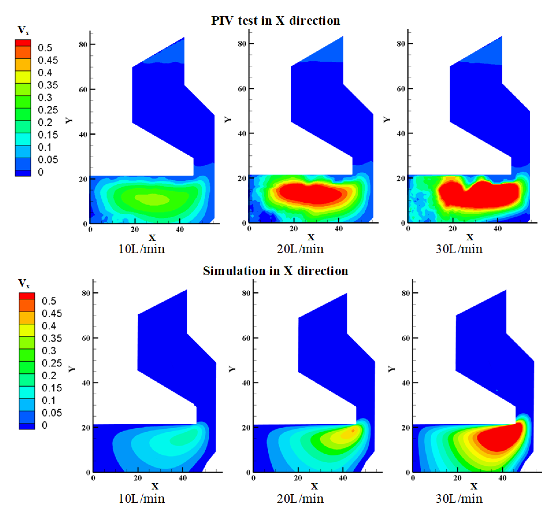
Figure 1. CFD model of the hydrodynamic retarder discharging valve.
Machines 11 00460 g001
Figure 2. Mesh size and flow rate and time consumption.
Machines 11 00460 g002
Figure 3. PIV experimental equipment and arrangement.
Machines 11 00460 g003
Figure 4. Comparison of PIV test results with simulation results in X direction.
Machines 11 00460 g004
Figure 5. Comparison of PIV test results with simulation results in Y direction.
Machines 11 00460 g005
Figure 6. Process of deep learning flow field construction.
Machines 11 00460 g006
Figure 7. Architectures of Res-SE-U-Nets in flow field construction.
Machines 11 00460 g007
Figure 8. Res-SE block used in this study.
Machines 11 00460 g008
Figure 9. Discharging valve velocity field under different spool displacements: (a) h = 5 mm; (b) h = 10 mm; (c) h = 15 mm.
Machines 11 00460 g009
Figure 10. Discharging valve velocity field under different pressure differences. (a) Δ p = 4 bar; (b) Δ p = 6 bar; (c) Δ p = 8 bar.
Machines 11 00460 g010
Figure 11. Velocity field reconstruction in training set.
Machines 11 00460 g011
Figure 12. Velocity field reconstruction in test set.
Machines 11 00460 g012
Figure 13. Cross-section diagram of the discharging valve.
Machines 11 00460 g013
Figure 14. Extraction of location information in postprocessing reconstructed velocity field: (a) h = 7 mm; (b) h = 8 mm; (c) h = 9 mm; (d) h = 10 mm; (e) h = 11 mm; (f) h = 12 mm; (g) h = 13 mm; (h) h = 14 mm; (i) h = 15 mm.
Machines 11 00460 g014
Figure 15. Comparison of the results of different steady-state flow force calculation methods.
Machines 11 00460 g015
Figure 16. Comparison of error for different spool displacement: (a) h = 10 mm; (b) h = 11 mm.
Machines 11 00460 g016
Table 1. Correlation coefficient in different working condition.
Direction10 L/min20 L/min30 L/min
x0.670.600.73
y0.570.460.42
Table 2. The hyperparameters of Res-SE-U-Nets.
No.LayerKernelStridePaddingFunction
1Convolutional layer220Sigmoid
2Convolutional layer220ReLU
3Convolutional layer221ReLU
4Transposed convolutional layer331ReLU
5Transposed convolutional layer220ReLU
6Transposed convolutional layer221ReLU
7Convolutional layer + Batch Normalization---ReLU
8Global pooling layer----
9Fully connected layer---ReLU
10Fully connected layer---Sigmoid
Disclaimer/Publisher’s Note: The statements, opinions and data contained in all publications are solely those of the individual author(s) and contributor(s) and not of MDPI and/or the editor(s). MDPI and/or the editor(s) disclaim responsibility for any injury to people or property resulting from any ideas, methods, instructions or products referred to in the content.

