
Yaw Rate Prediction and Tilting Feedforward Synchronous Control of Narrow Tilting Vehicle Based on RNN
 ,
,
Abstract
1. Introduction
- (1)
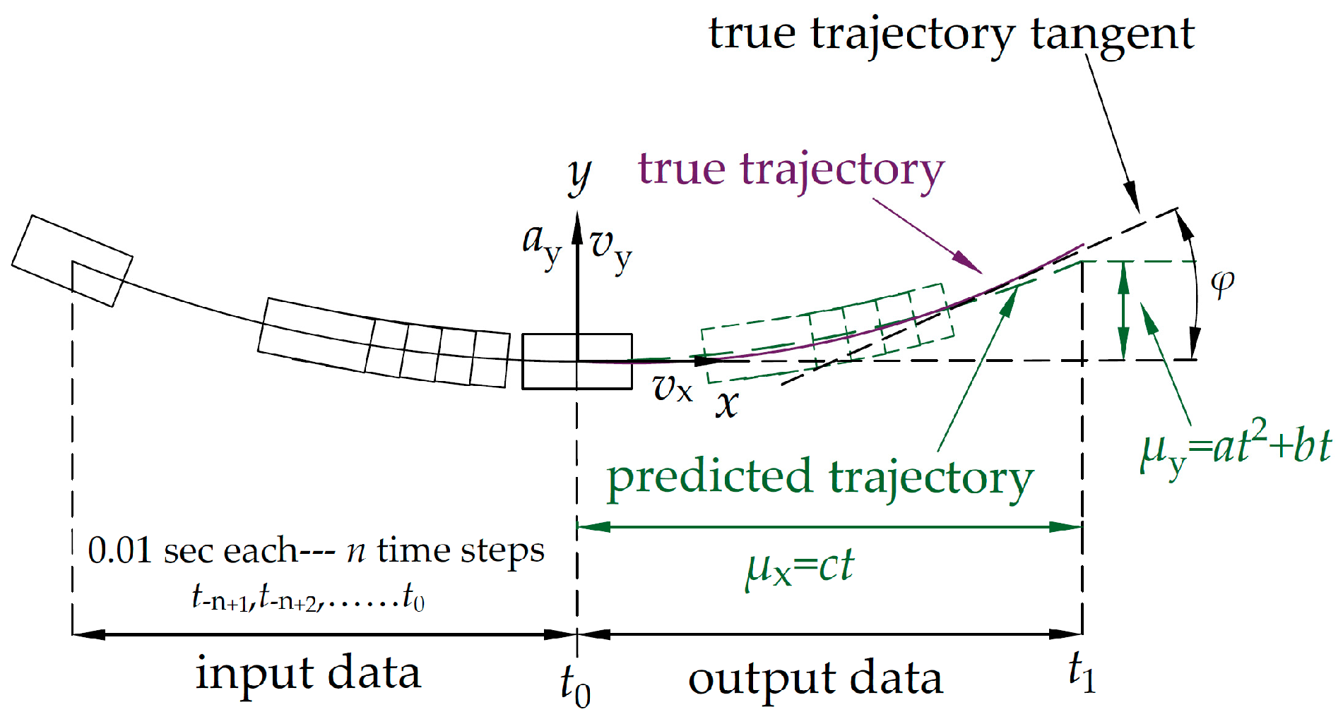
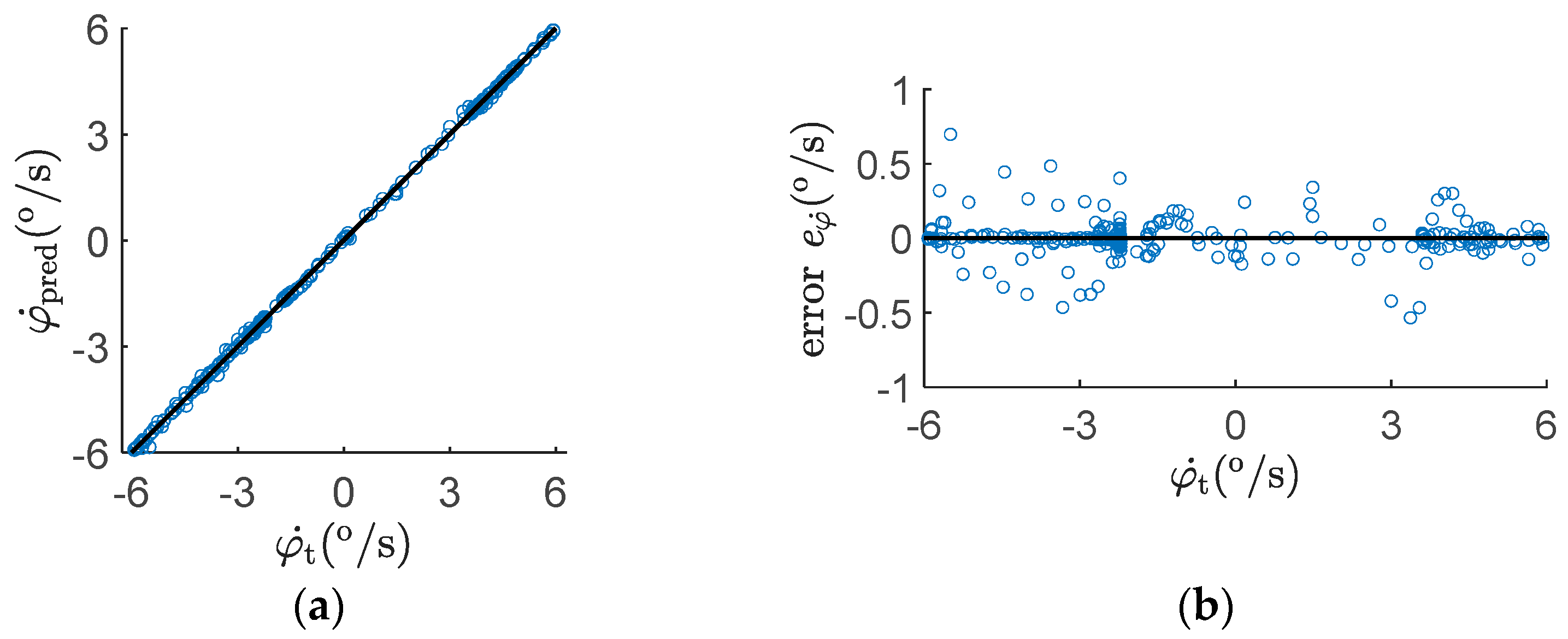
- A calculating method for predicting the yaw rate is proposed. The NTV yaw rate is represented by a polynomial operation to predict the continuous yaw rate in the time domain.
- (2)
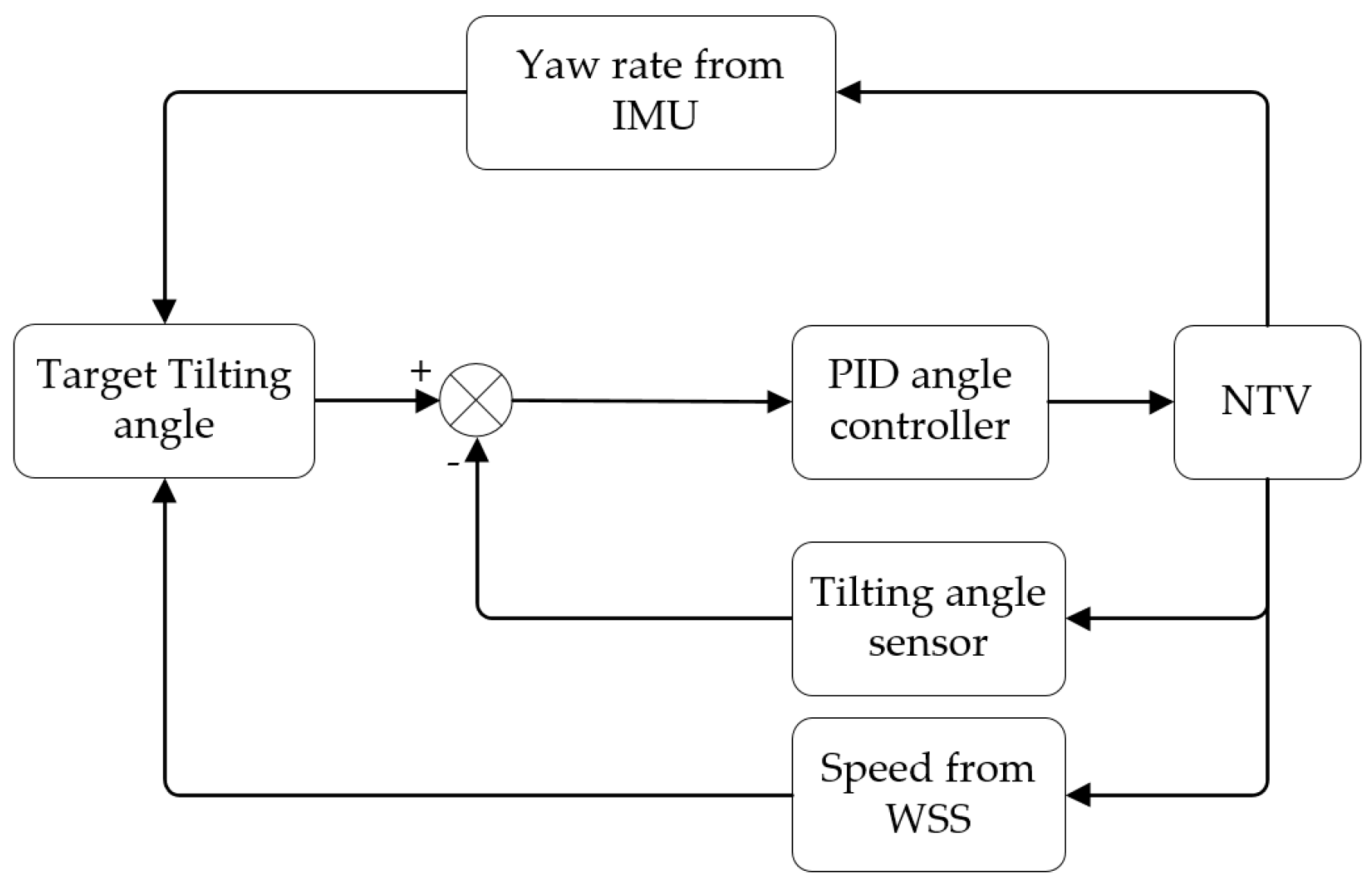
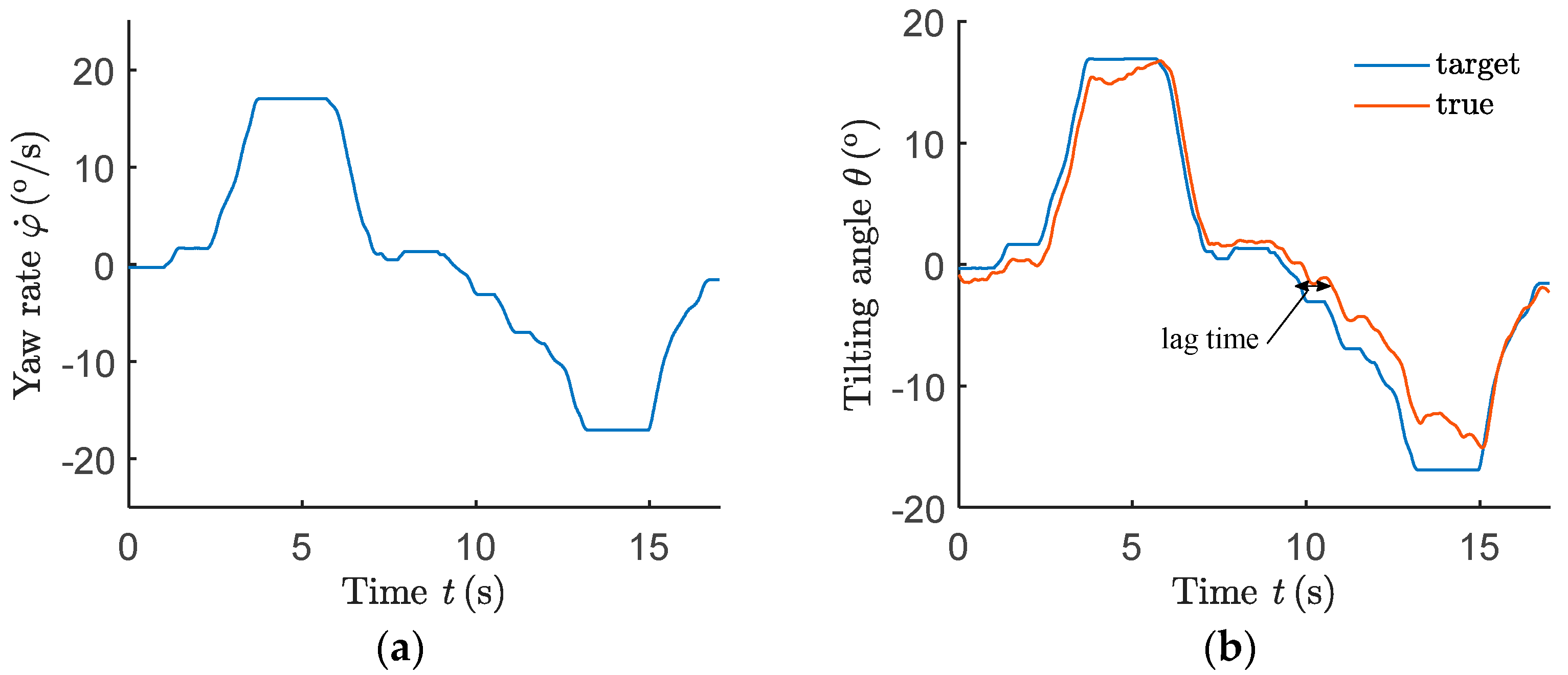
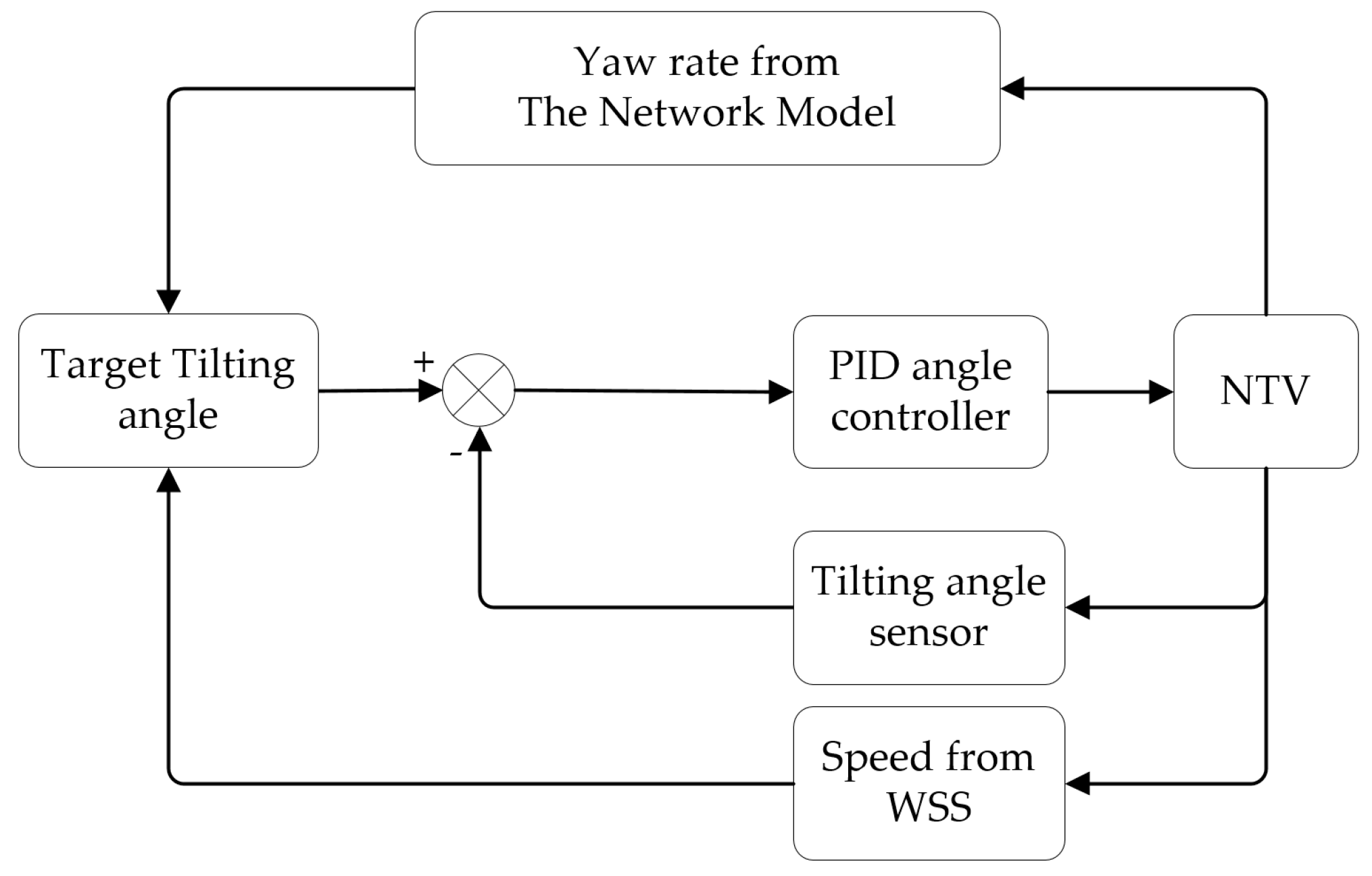
- The tilting feedforward synchronous control (TFSC) method for NTVs based on the predicted value of the yaw rate is proposed.
- (3)
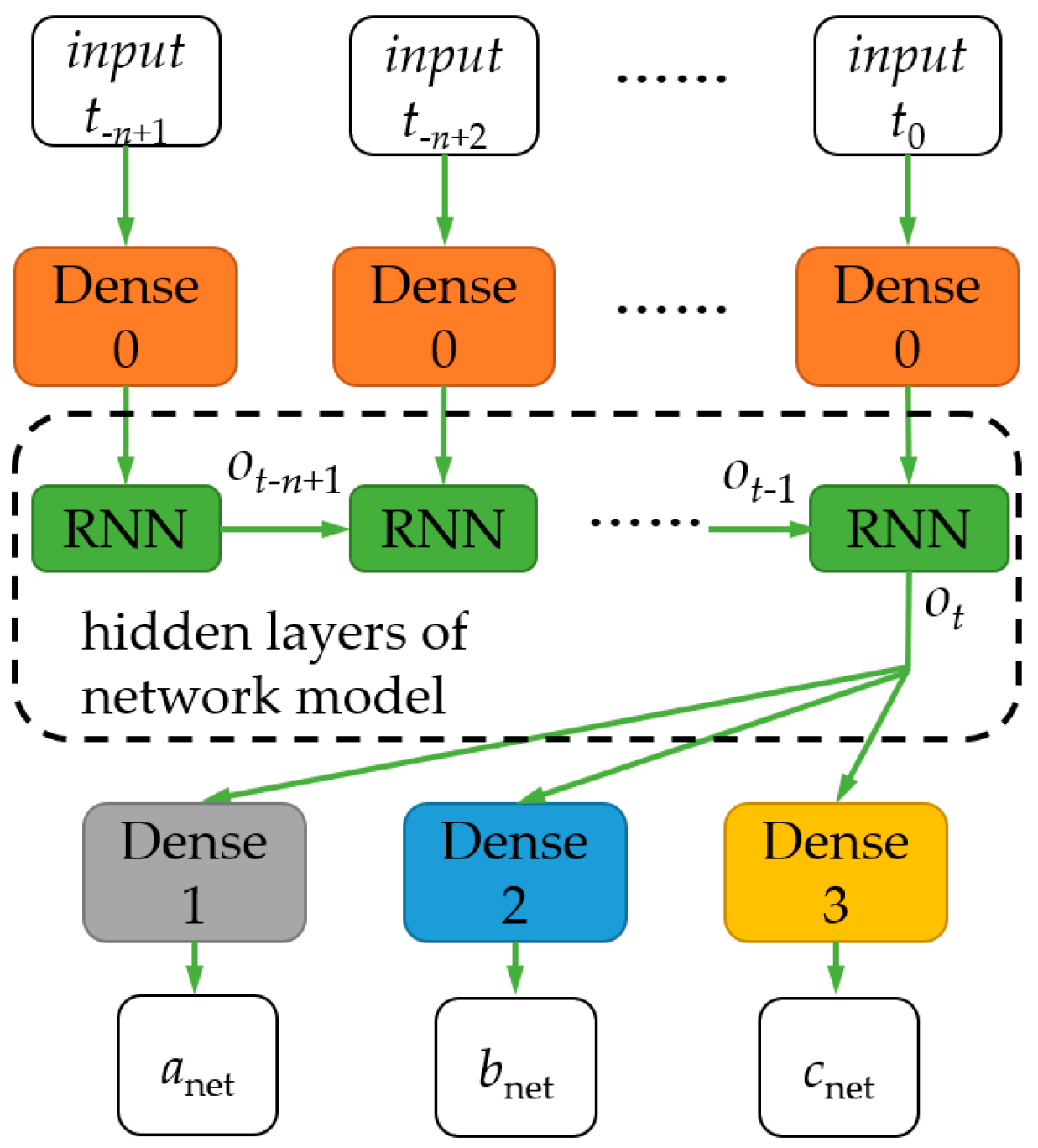
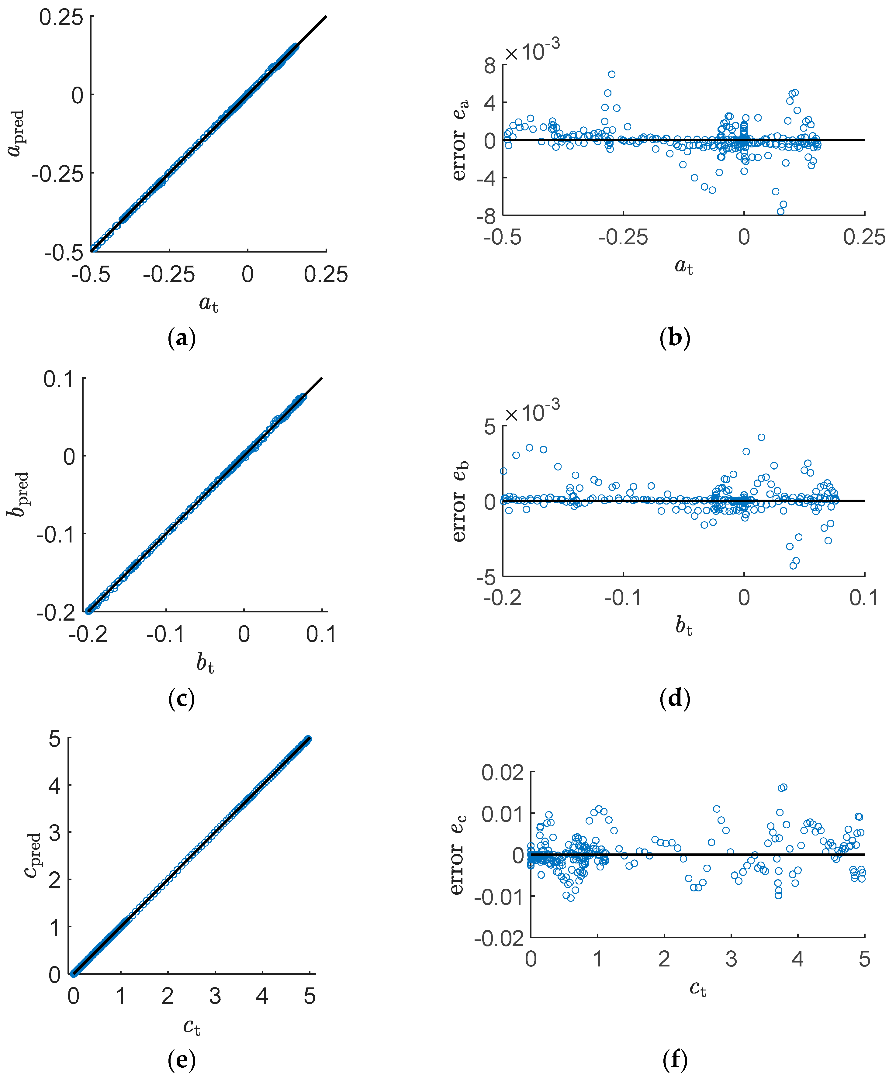
- A network model is designed based on RNN to predict the coefficients of the polynomial operation. The model is trained on real driving data collected by an NTV prototype.
- (4)
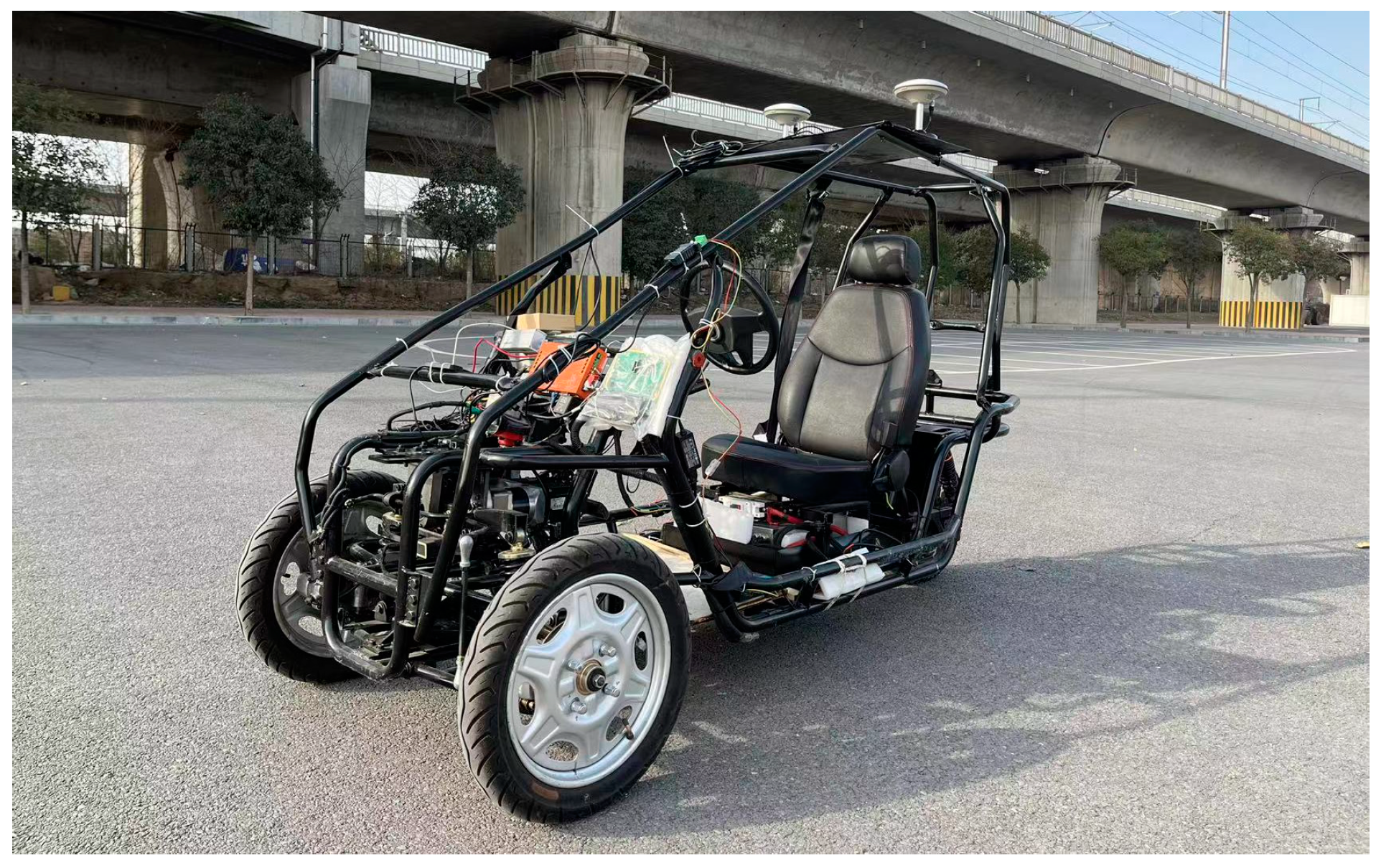
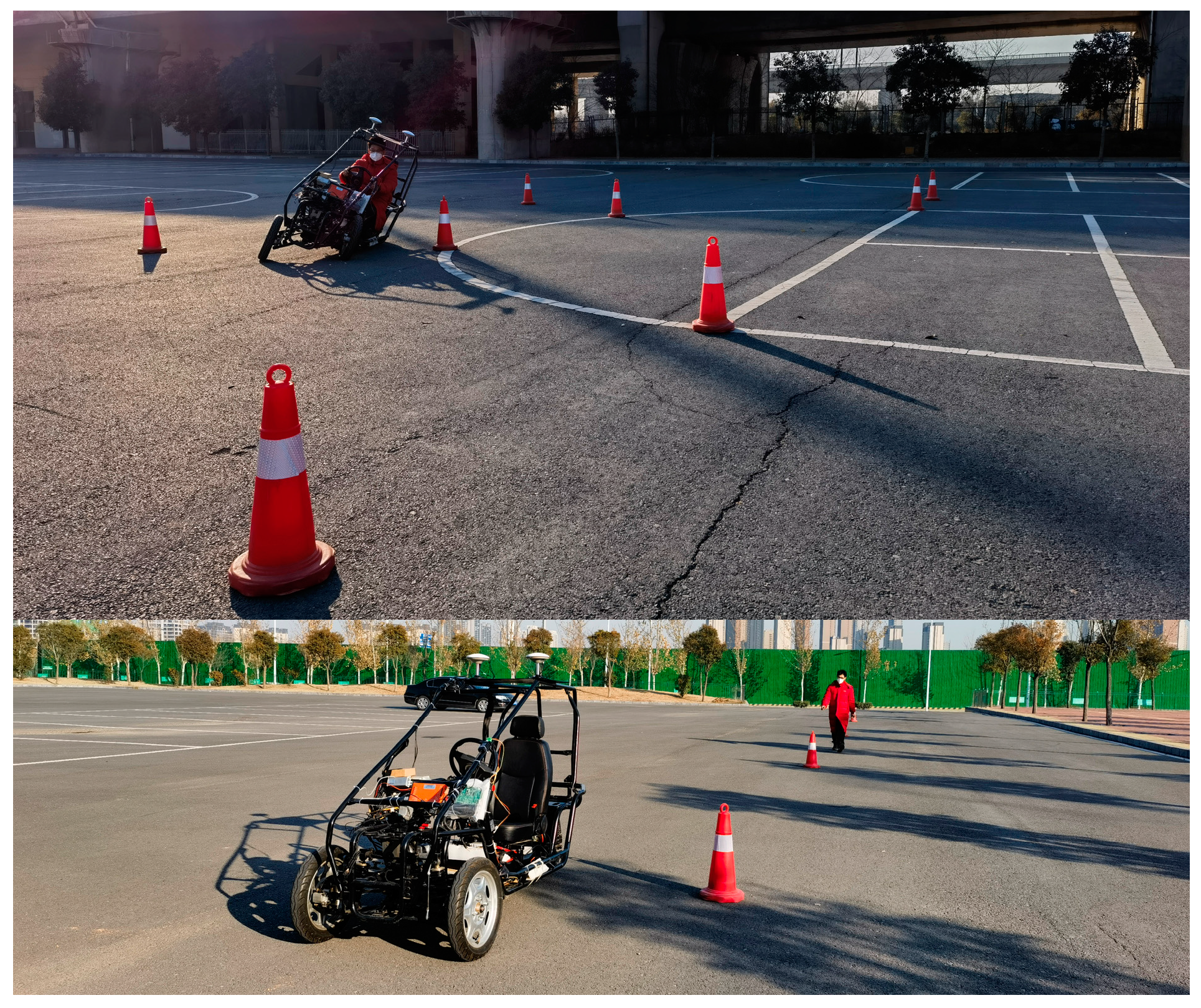
- The NTV prototype is used to collect vehicle driving data, and the network model works entirely with data obtained from onboard sensors. The feasibility of the TFSC method is verified by the prototype experiment.
2. Mathematics and Network Model for Prediction
2.1. Mathematics, Input, and Output
2.2. Network Model
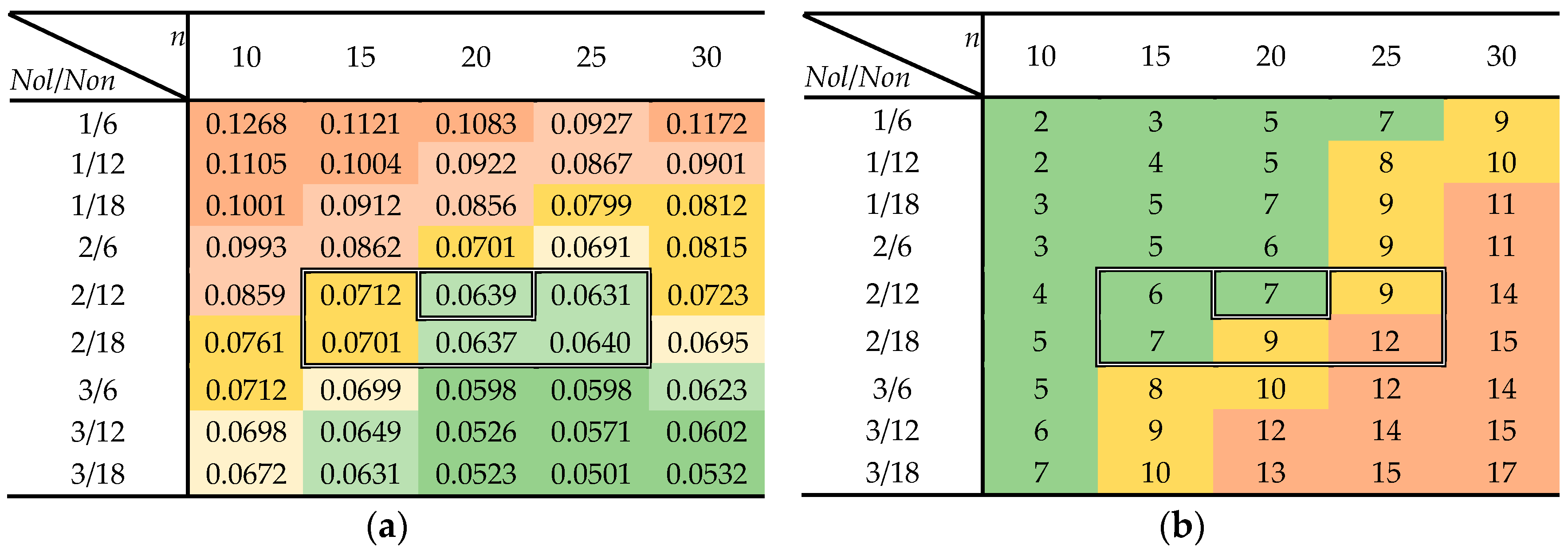
2.3. Training
3. Tilting Feedforward Synchronous Control
4. Experiments
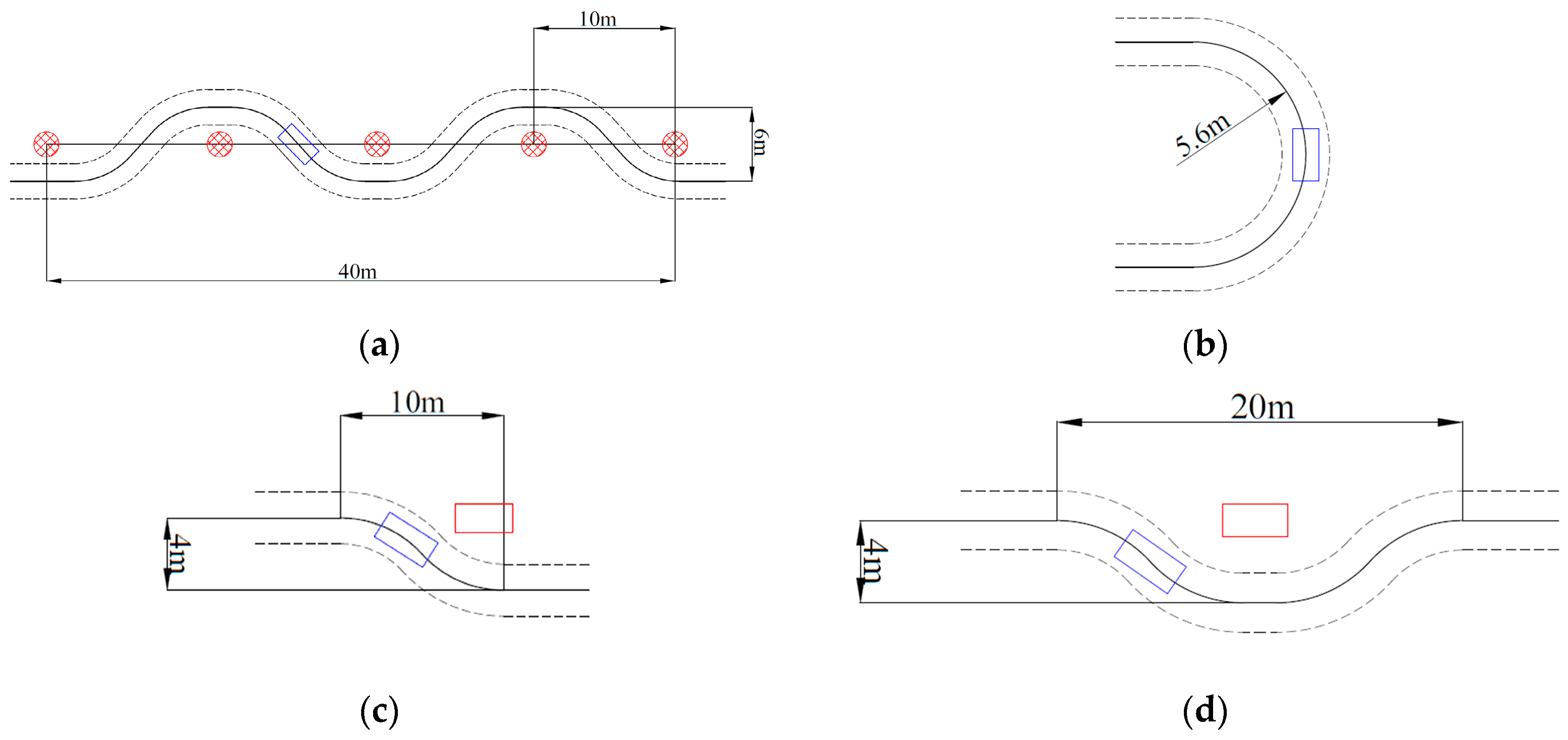
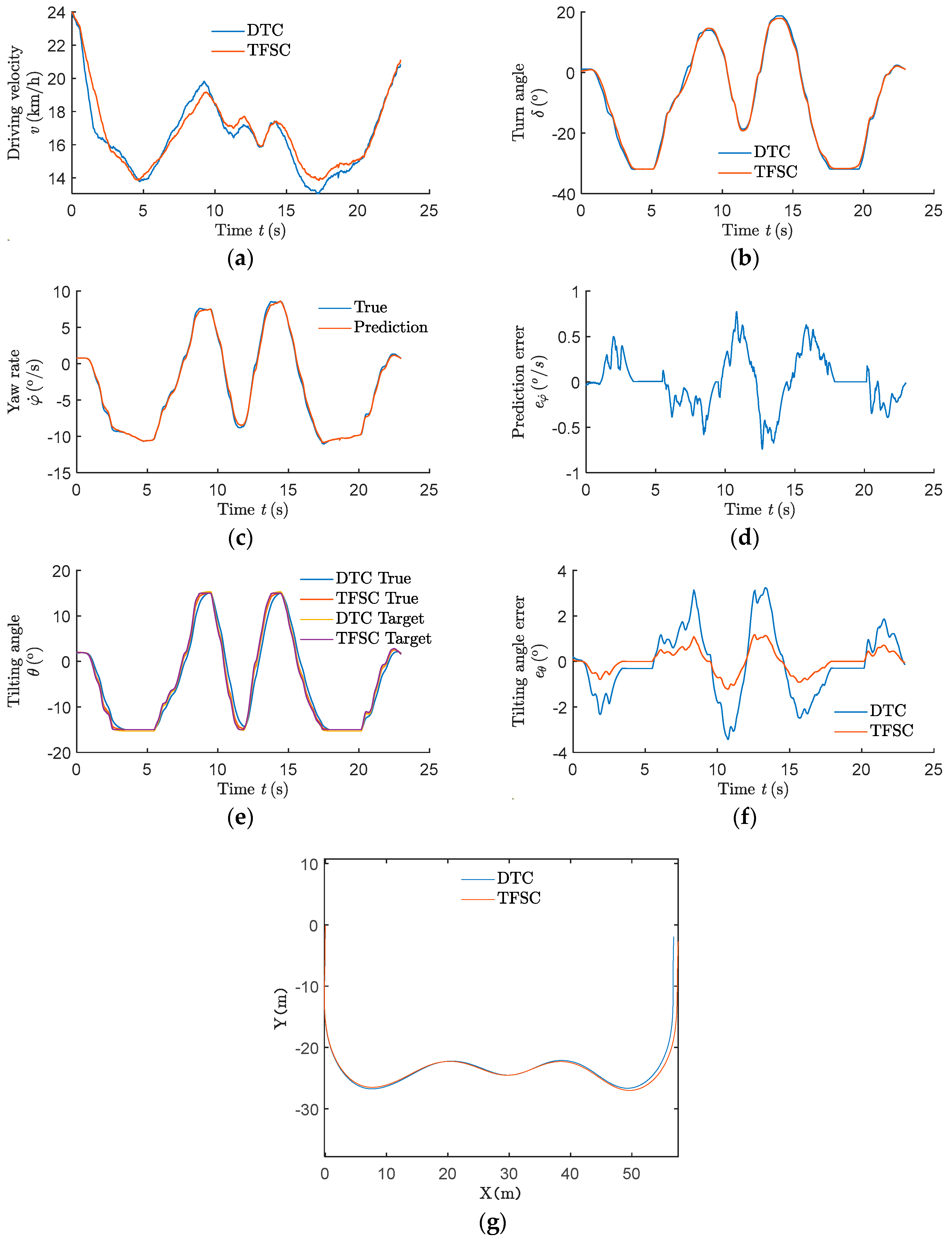
4.1. “S”-Type Route Experiment
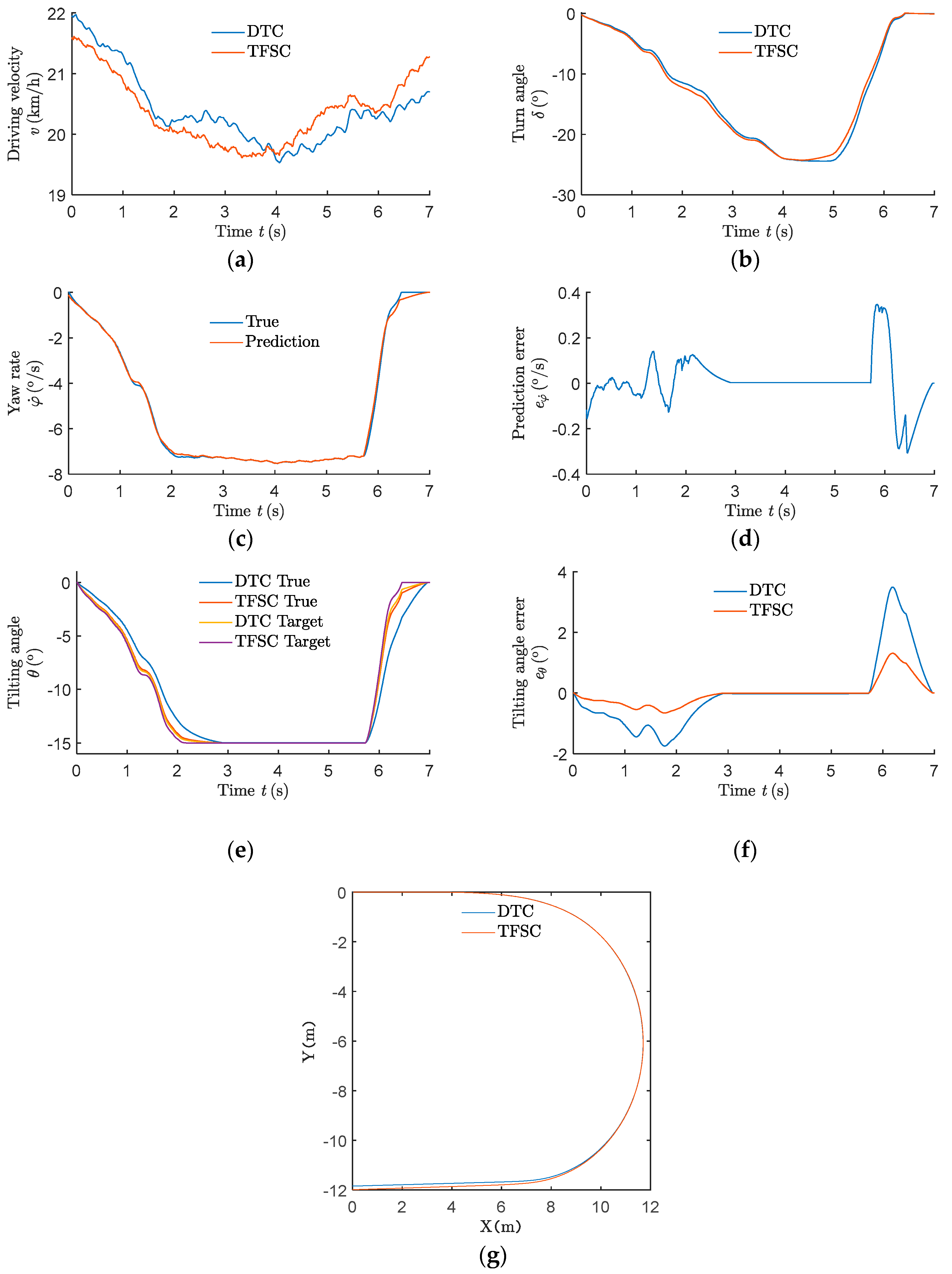
4.2. “C”-Type Route Experiment
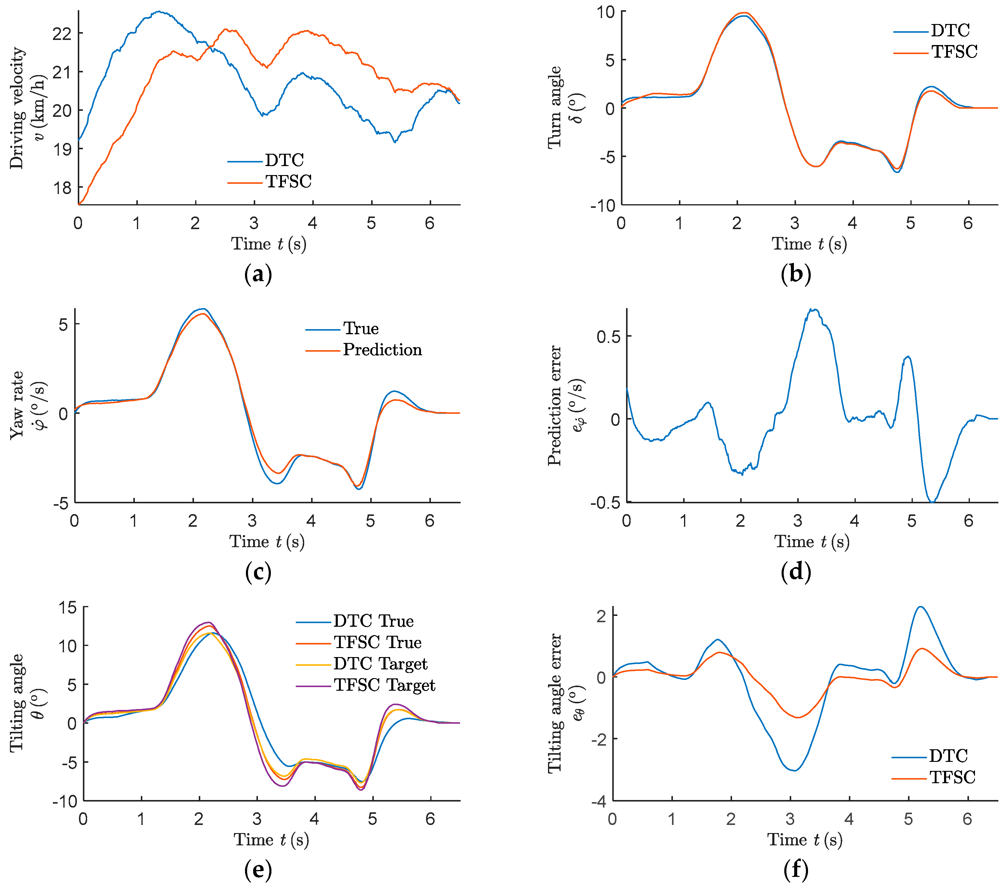
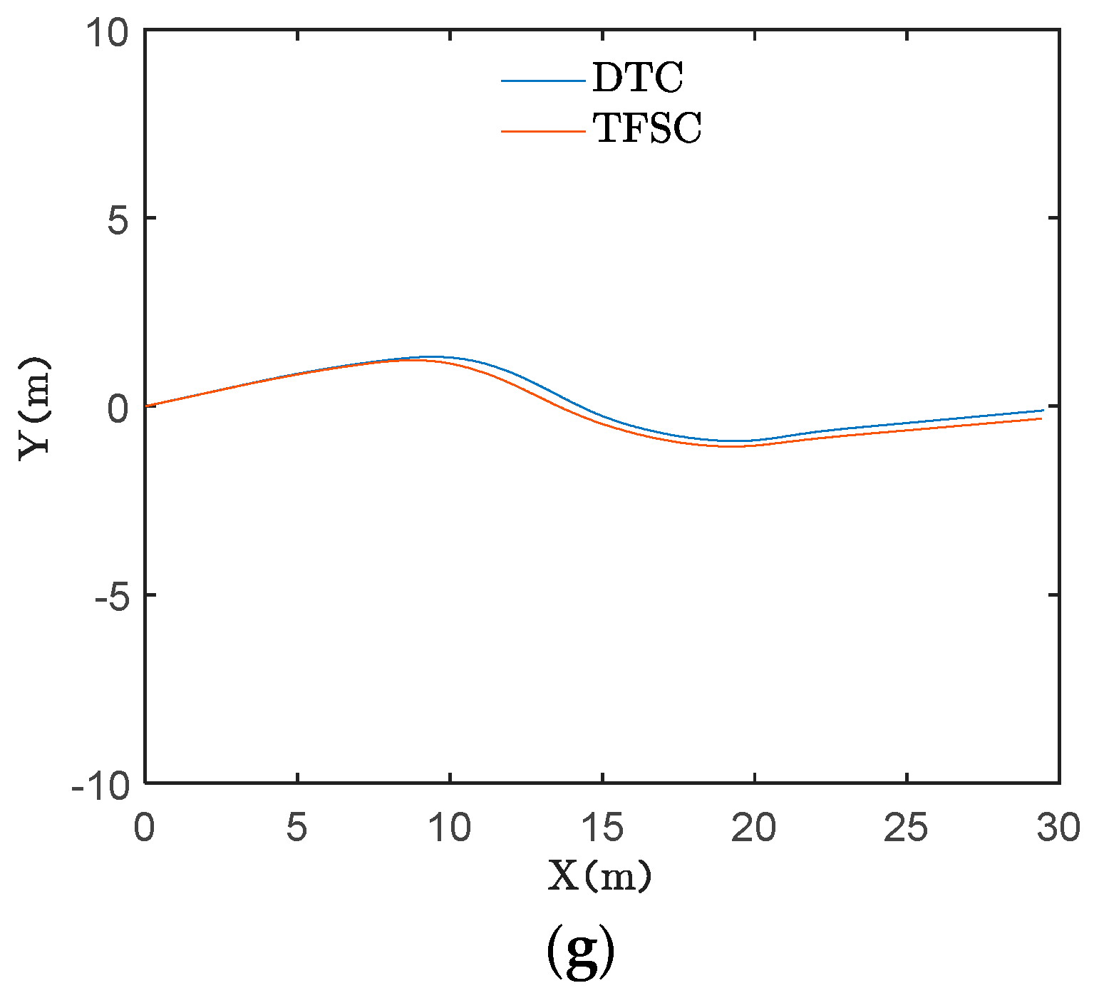
4.3. Single Lane Change Route Experiment
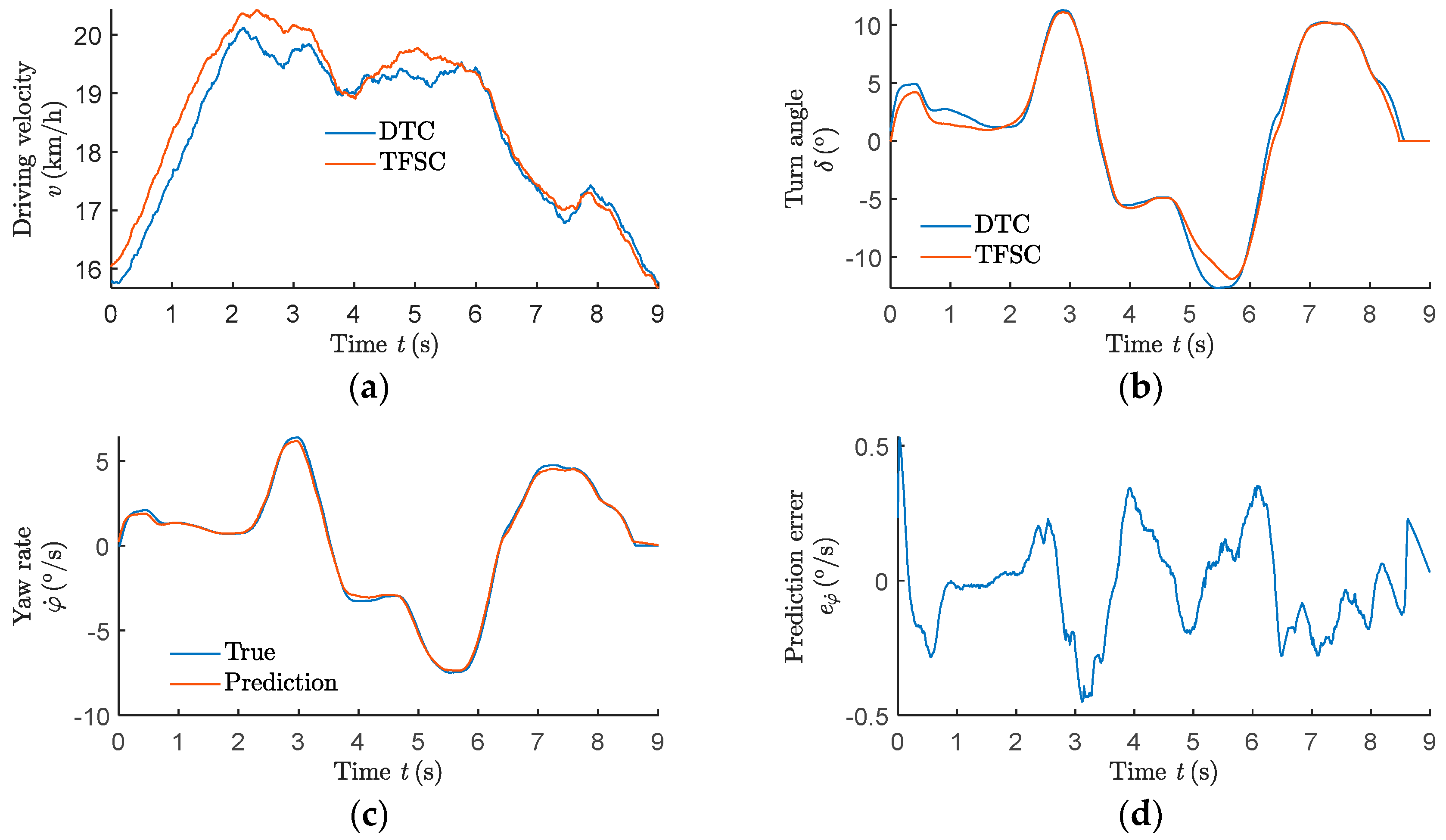
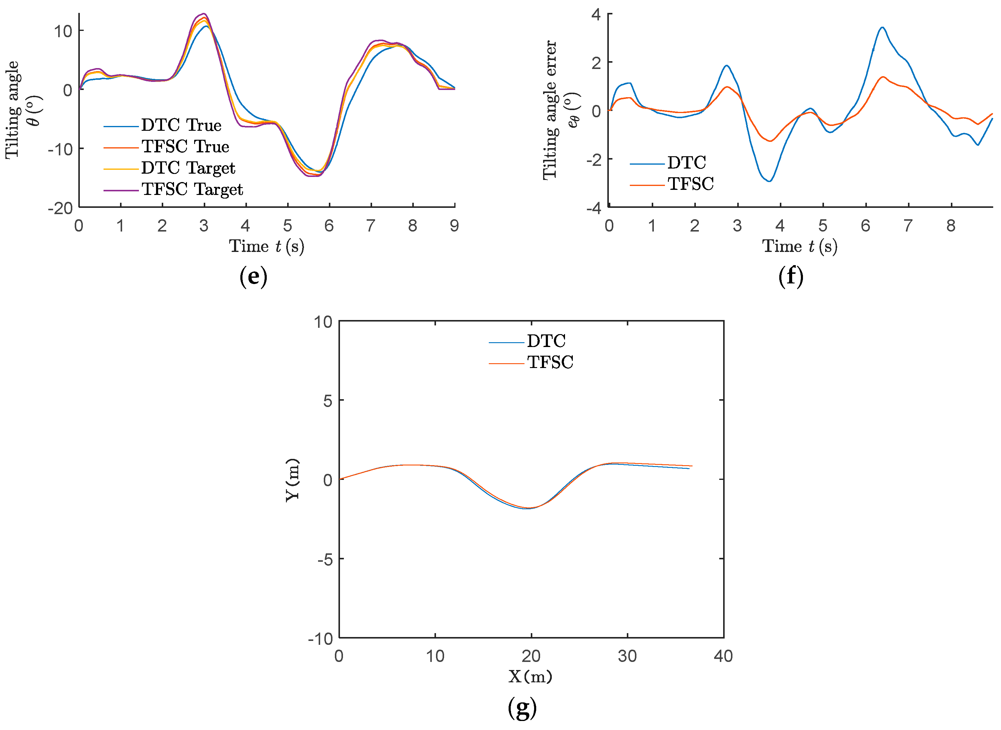
4.4. Double Lane Change Route Experiment
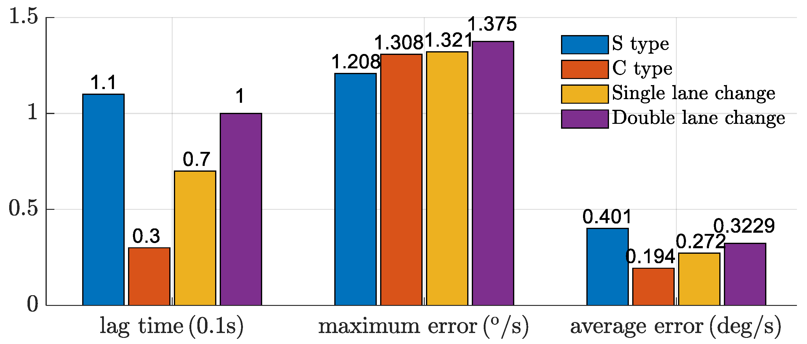
4.5. Analysis of Experiment Results
5. Discussion
6. Conclusions
7. Patents
Author Contributions
Funding
Data Availability Statement
Acknowledgments
Conflicts of Interest
References
- Xu, D.; Han, Y.; Han, X.; Wang, Y.; Wang, G. Narrow Tilting Vehicle Drifting Robust Control. Machines 2023, 11, 90. [Google Scholar] [CrossRef]
- Hibbard, R.; Karnopp, D. Twenty First Century Transportation System Solutions—A New Type of Small, Relatively Tall and Narrow Active Tilting Commuter Vehicle. Veh. Syst. Dyn. 1996, 25, 321–347. [Google Scholar] [CrossRef]
- Haraguchi, T.; Kageyama, I.; Kaneko, T. Study of Personal Mobility Vehicle (PMV) with Active Inward Tilting Mechanism on Obstacle Avoidance and Energy Efficiency. Appl. Sci. 2019, 9, 4737. [Google Scholar] [CrossRef]
- Ren, Y. Modelling and Control of Narrow Tilting Vehicle for Future Transportation System. In Intelligent and Efficient Transport Systems; IntechOpen: London, UK, 2020; p. 133. [Google Scholar]
- Nguyen, A.-T.; Chevrel, P.; Claveau, F. LPV Static Output Feedback for Constrained Direct Tilt Control of Narrow Tilting Vehicles. IEEE Trans. Control Syst. Technol. 2020, 28, 661–670. [Google Scholar] [CrossRef]
- Gao, R.L.; Li, H.T.; Wei, W.J.; Wang, Y. Research on the Decoupling of the Parallel Vehicle Tilting and Steering Mechanism. Appl. Sci. 2022, 12, 7502. [Google Scholar] [CrossRef]
- Wang, Y.; Wei, W. Vehicle Steering Tilting Linkage Device and Active Tilting Vehicle. CN 109625087 A, 16 April 2019. [Google Scholar]
- Liu, P.; Li, X.; Gao, R.; Li, H.; Wei, W.; Wang, Y. Design and experiment of tilt-driving mechanism for the vehicle. J. Jilin Univ. 2022, 1, 1–8. [Google Scholar] [CrossRef]
- Liu, P.; Ke, C.; Gao, R.; Li, H.; Wei, W.; Wang, Y. Design and Test of Active Roll Vehicle. Automot. Eng. 2020, 42, 1552–1557+1584. [Google Scholar] [CrossRef]
- Mourad, L.; Claveau, F.; Chevrel, P. Direct and Steering Tilt Robust Control of Narrow Vehicles. IEEE Trans. Intell. Transp. Syst. 2014, 15, 1206–1215. [Google Scholar] [CrossRef]
- Claveau, F.; Chevrel, P.; Mourad, L. Non-linear control of a narrow tilting vehicle. In Proceedings of the 2014 IEEE International Conference on Systems, Man, and Cybernetics (SMC), San Diego, CA, USA, 5–8 October 2014; pp. 2488–2494. [Google Scholar]
- Tang, C.; Khajepour, A. Integrated Stability Control for Narrow Tilting Vehicles: An Envelope Approach. IEEE Trans. Intell. Transp. Syst. 2021, 55, 3158–3166. [Google Scholar] [CrossRef]
- Tang, C.; Ataei, M.; Khajepour, A. A Reconfigurable Integrated Control for Narrow Tilting Vehicles. IEEE Trans. Veh. Technol. 2019, 68, 234–244. [Google Scholar] [CrossRef]
- Ataei, M. Reconfigurable Integrated Control for Urban Vehicles with Different Types of Control Actuation. Doctoral Thesis, University of Waterloo, Waterloo, ON, Canada, 2017. [Google Scholar]
- Snell, A. An active roll-moment control strategy for narrow tilting commuter vehicles. Veh. Syst. Dyn. 1998, 29, 277–307. [Google Scholar] [CrossRef]
- Chong, J.; Marco, J.; Greenwood, D. Modelling and simulations of a narrow track tilting vehicle. Exch. Interdiscip. Res. J. 2016, 4, 86–105. [Google Scholar] [CrossRef]
- Li, H.; Gao, R.; Li, X.; Zhang, J.; Wang, Y.; WEI, W. Vehicle Tilting Control Method. CN 111231935 A, 13 January 2020. [Google Scholar]
- Gao, J.; Sun, C.; Zhao, H.; Shen, Y.; Anguelov, D.; Li, C.; Schmid, C. Vectornet: Encoding hd maps and agent dynamics from vectorized representation. In Proceedings of the IEEE/CVF Conference on Computer Vision and Pattern Recognition, Seattle, WA, USA, 13–19 June 2020; pp. 11525–11533. [Google Scholar]
- Houenou, A.; Bonnifait, P.; Cherfaoui, V.; Yao, W. Vehicle trajectory prediction based on motion model and maneuver recognition. In Proceedings of the 2013 IEEE/RSJ International Conference on Intelligent Robots and Systems, Tokyo, Japan, 3–7 November 2013; pp. 4363–4369. [Google Scholar]
- Patel, S.; Griffin, B.; Kusano, K.; Corso, J.J. Predicting Future Lane Changes of Other Highway Vehicles using RNN-Based Deep Models. arXiv 2018, arXiv:1801.04340. [Google Scholar]
- Liu, W.; Shoji, Y. DeepVM: RNN-Based Vehicle Mobility Prediction to Support Intelligent Vehicle Applications. IEEE Trans. Ind. Inform. 2020, 16, 3997–4006. [Google Scholar] [CrossRef]
- Min, K.; Kim, D.; Park, J.; Huh, K. RNN-Based Path Prediction of Obstacle Vehicles with Deep Ensemble. IEEE Trans. Veh. Technol. 2019, 68, 10252–10256. [Google Scholar] [CrossRef]
- Kim, J.-H.; Kum, D.-S. Threat prediction algorithm based on local path candidates and surrounding vehicle trajectory predictions for automated driving vehicles. In Proceedings of the 2015 IEEE Intelligent Vehicles Symposium (IV), Seoul, Republic of Korea, 28 June–1 July 2015; pp. 1220–1225. [Google Scholar]
- Kang, C.M.; Jeon, S.J.; Lee, S.-H.; Chung, C.C. Parametric trajectory prediction of surrounding vehicles. In Proceedings of the 2017 IEEE International Conference on Vehicular Electronics and Safety (ICVES), Vienna, Austria, 27–28 June 2017; pp. 26–31. [Google Scholar]
- Battauz, M.; Vidoni, P. A likelihood-based boosting algorithm for factor analysis models with binary data. Comput. Stat. Data Anal. 2022, 168, 107412. [Google Scholar] [CrossRef]
- Pang, Y.; Shi, M.; Zhang, L.; Song, X.; Sun, W. PR-FCM: A polynomial regression-based fuzzy C-means algorithm for attribute-associated data. Inf. Sci. 2022, 585, 209–231. [Google Scholar] [CrossRef]
- Bi, Z.; Xu, G.; Xu, G.; Wang, C.; Zhang, S. Bit-Level Automotive Controller Area Network Message Reverse Framework Based on Linear Regression. Sensors 2022, 22, 981. [Google Scholar] [CrossRef] [PubMed]
- Zhang, S.; Li, D.; Du, F.; Wang, T.; Liu, Y. Prediction of Vehicle Braking Deceleration Based on BP Neural Network. J. Phys. Conf. Ser. 2022, 2183, 012025. [Google Scholar] [CrossRef]
- Lee, T.-H.; Ullah, A.; Wang, R. Bootstrap Aggregating and Random Forest. In Macroeconomic Forecasting in the Era of Big Data; Springer Nature Switzerland AG: Cham, Switzerland, 2019; pp. 389–429. [Google Scholar]
- Gao, R.; Li, H.; Zhang, J.; Wang, Y.; Wei, W.; Wang, B. Research on Steering Comfort of Active Tilting Vehicles. In Proceedings of the 2021 China SAE Congress and Exhibition (SAECCE), Shanghai, China, 19–21 October 2021. [Google Scholar]
- Zhang, J.; Li, H.; Gao, R.; Wang, Y.; Wei, W.; Wang, B. Research and Test on the Stability of Active Rollover Three-wheeled Vehicle. In Proceedings of the 2021 China SAE Congress and Exhibition (SAECCE), Shanghai, China, 19–21 October 2021. [Google Scholar]
- GB/T 6323-2014; Controllability and Stability Test Procedure for Automobile. General Administration of Quality Supervision, Inspection and Quarantine of the People’s Republic of China: Beijing, China, 2014.
- Yao, J.; Wang, M.; Li, Z.; Jia, Y. Research on model predictive control for automobile active tilt based on active suspension. Energies 2021, 14, 671. [Google Scholar] [CrossRef]


| Maximum Absolute Error (°) | Average Absolute Error (°) | Average Lag Time (s) | |
|---|---|---|---|
| DTC | 3.317 | 1.179 | 0.21 |
| TFSC | 1.208 | 0.401 | 0.11 |
| Maximum Absolute Error (°) | Average Absolute Error (°) | Average Lag Time (s) | |
|---|---|---|---|
| DTC | 3.488 | 0.5167 | 0.07 |
| TFSC | 1.308 | 0.1938 | 0.03 |
| Maximum Absolute Error (°) | Average Absolute Error (°) | Average Lag Time (s) | |
|---|---|---|---|
| DTC | 3.029 | 0.5963 | 0.16 |
| TFSC | 1.321 | 0.2716 | 0.07 |
| Maximum Absolute Error (°) | Average Absolute Error (°) | Average Lag Time (s) | |
|---|---|---|---|
| DTC | 3.409 | 0.7089 | 0.18 |
| TFSC | 1.375 | 0.3229 | 0.10 |
Disclaimer/Publisher’s Note: The statements, opinions and data contained in all publications are solely those of the individual author(s) and contributor(s) and not of MDPI and/or the editor(s). MDPI and/or the editor(s) disclaim responsibility for any injury to people or property resulting from any ideas, methods, instructions or products referred to in the content. |
© 2023 by the authors. Licensee MDPI, Basel, Switzerland. This article is an open access article distributed under the terms and conditions of the Creative Commons Attribution (CC BY) license (https://creativecommons.org/licenses/by/4.0/).
Share and Cite
Gao, R.; Li, H.; Wang, Y.; Xu, S.; Wei, W.; Zhang, X.; Li, N. Yaw Rate Prediction and Tilting Feedforward Synchronous Control of Narrow Tilting Vehicle Based on RNN. Machines 2023, 11, 370. https://doi.org/10.3390/machines11030370
Gao R, Li H, Wang Y, Xu S, Wei W, Zhang X, Li N. Yaw Rate Prediction and Tilting Feedforward Synchronous Control of Narrow Tilting Vehicle Based on RNN. Machines. 2023; 11(3):370. https://doi.org/10.3390/machines11030370
Chicago/Turabian StyleGao, Ruolin, Haitao Li, Ya Wang, Shaobing Xu, Wenjun Wei, Xiao Zhang, and Na Li. 2023. "Yaw Rate Prediction and Tilting Feedforward Synchronous Control of Narrow Tilting Vehicle Based on RNN" Machines 11, no. 3: 370. https://doi.org/10.3390/machines11030370
APA StyleGao, R., Li, H., Wang, Y., Xu, S., Wei, W., Zhang, X., & Li, N. (2023). Yaw Rate Prediction and Tilting Feedforward Synchronous Control of Narrow Tilting Vehicle Based on RNN. Machines, 11(3), 370. https://doi.org/10.3390/machines11030370