Article

A Novel Rolling Bearing Fault Diagnosis Method Based on BLS and CNN with Attention Mechanism

1
School of Management, Hefei University of Technology, Hefei 230009, China
2
School of Software, Tsinghua University, Beijing 100084, China
*
Author to whom correspondence should be addressed.
Machines 2023, 11(2), 279; https://doi.org/10.3390/machines11020279
Submission received: 17 November 2022 / Revised: 4 February 2023 / Accepted: 8 February 2023 / Published: 13 February 2023
(This article belongs to the Section Machines Testing and Maintenance)

Abstract

:
In actual industrial application scenarios, noise pollution makes it difficult to extract fault features accurately via conventional methods. A novel method for rolling bearing fault diagnosis combining a convolutional neural network (CNN), an attention mechanism for a squeeze-and-excitation network (SENet) module and a broad learning system (BLS) is proposed (SECNN–BLS). The one-dimensional bearing vibration signal is processed by using multiple short-time Fourier transforms (STFT); the two-dimensional image in the time-frequency domain is used as the model input. In the CNN fault feature extraction process, SENet is introduced to replace the CNN convolution layer, and global information is obtained through the squeeze operation. Excitation operation captures the importance of image channels, assigns weights adaptively to improve the attention on important information and eliminates the interference of irrelevant features without increasing the spatial and temporal complexity. The weighted feature representation is then transferred to the BLS input. The BLS has the characteristics of a flat structure and ridge regression to quickly solve the weights; as a fault classifier, it can save more computing resources and improve the accuracy of the fault classification. The SECNN–BLS fault diagnosis has achieved more than 98% accuracy on the Society for Machinery Failure Prevention Technology (MFPT) dataset. We also demonstrate the excellent performance of SECNN–BLS in a noisy environment.

1. Introduction

Against the background of intelligent manufacturing, rotating machinery equipment—an important part of the manufacturing industry—is developing in the direction of intelligence, informatization and automation. Its structure and function are becoming more sophisticated and complex to meet growing industrial needs [1]. Due to its continuous high-speed operation during the production process, the bearing is often subject to equipment wear and aging, which is one of the causes of safety accidents [2]. Untimely processing and poor judgment may result in equipment damage and even injuries, causing the entire production system to stagnate and affecting manufacturing efficiency. Therefore, effective fault diagnosis is essential to ensure the reliability of system operations.
At present, bearing fault diagnosis technology includes the analysis of temperature, vibration, ultrasound, static electricity, etc. [3]. The vibration signal is the most commonly used of these, due to easy data acquisition and analysis. In addition, when the surface of a rolling bearing is partially damaged, the bearing will generate a periodic broadband pulse excitation signal, making it effective and convenient to analyze the vibration signal of the rolling bearing. Fault feature extraction and state classification are the key steps of data-driven intelligent fault diagnosis methods. The current methods for feature extraction from rolling bearing vibration signals include analysis of the time domain, frequency domain and time-frequency domain. Time-frequency domain analysis of vibration signals is widely used of these, as are wavelet transform [4], empirical mode decomposition [5], local mean decomposition [6] and so on. The extracted features are used to identify fault states through shallow machine learning algorithms such as random forests [7]. However, these methods rely on specific domain knowledge, cannot learn deep-level features and do not have sufficient generalization ability to address scenarios with high integration and complex working conditions.
Due to its powerful automatic learning ability and improved classification accuracy, deep learning has now been developing rapidly and improving continuously. This data-driven method can better adapt to massive high-dimensional heterogeneous data; the non-linear processing units in the deep structure enable more accurate feature extraction and abstract modeling. Among these methods, CNN is currently the most representative in rolling bearing diagnosis, owing to characteristics of translation invariant classification, weight sharing and convolution calculation. Guo et al. [8] proposed a method for multi-task CNN with information fusion and adopted dynamic training, which can simultaneously complete fault diagnosis and localization. Gao et al. [9] combined CNN with parameter optimization maximum correlated kurtosis deconvolution (MCKD) to address the difficulty of feature extraction for faulty signals in noisy backgrounds.
Although CNN has achieved excellent results in fault diagnosis, it is not easy to adapt it to the changeable load and system environment in actual industrial scenarios. The attention mechanism, an important concept in deep learning, involves adaptively extracting features according to their importance, thereby improving the contribution of important features to the model. Wang et al. [10] proposed a multi-attention 1DCNN fault diagnosis model, which can enhance fault-related features adaptively and improve discriminative feature representation. Xu et al. [11] combined the attention mechanism feature with an improved multi-scale CNN, which enhanced the anti-interference ability of the model.
Despite the popularity of deep-learning applications, they are limited by high training cost, necessitated by the large volume of sample data and fixed structure, which cannot adapt well to demand. The emergence of BLS has greatly improved this problem. When first proposed in 2018 [12], BLS consisted of input data, feature layer, an enhancement layer and output (output is the label corresponding to input data). BLS enriches the content of machine learning and expands the form of network neuron structures. Incremental learning is the core of BLS [13], having the advantage of accommodating increasing data without recalculating. Simultaneously, BLS can update the model efficiently, using the simple linear structure to reduce the computational complexity and workload, handling small batch data with ease [14]. Meanwhile, the flat simple linear structure makes BLS easy to reshape and integrate. Since BLS was proposed, endless structural variations have emerged and play a vital role in many fields [15]. The adaptive BLS method has been applied to fault diagnosis in rotating machinery [16]; in [17], BLS combined with principal component analysis was used for a high-speed train traction system.
Therefore, a novel method for fault diagnosis of rolling bearings based on CNN with SENet and BLS (SECNN–BLS) is proposed, which extracts features from sample data by CNN and introduces the SENet attention mechanism in the CNN feature extraction process in order to improve attention to discriminative features. The resulting feature map is then directly constructed into the BLS feature layer; finally, the BLS is trained to generate a fault classification. The contributions of this paper are summarized as follows:
(1) A fault diagnosis model integrating CNN and BLS with an attention mechanism is established. This method combines the advantages of CNN convolution calculation, deep sample feature extraction, the lightweight structure of SENet and the high efficiency of the BLS training model. In the feature extraction process of CNN, SENet is introduced to replace the convolution layer, which can expand from the local receptive field to the extraction of global feature information. In addition, the importance of image channels is captured through excitation operation in SENet; the weight is adaptively allocated to emphasize important feature information and reduce the interference of irrelevant information. BLS uses ridge regression to update the weight, which can improve calculation efficiency.
(2) The original vibration signal is processed by multiple short-time Fourier transforms and converted into the stereoscopic two-dimensional spectrum as the model input, which more intuitively retains the signal feature information and is conducive to SECNN–BLS feature extraction of the original information.
(3) The experimental results show that the SECNN–BLS fault diagnosis model has higher diagnosis accuracy and noise resistance than other methods under normal and noisy environments. It can better adapt to complex and changeable industrial scenarios.
The remaining content of this article is arranged as follows: The theoretical methods of CNN, BLS and the attention mechanism are introduced in Section 2. Section 3 describes the framework design and construction process of SECNN–BLS in detail. In Section 4, the MFPT dataset, experimental design scheme and performance metrics are introduced, as well as the analysis the final experimental results. Finally, Section 5 provides the conclusion and summarizes the shortcomings.

2. Related Work

In this section, the basic principles of CNN, BLS and attention mechanism theory are introduced. The method proposed in this paper combines the depth feature extraction advantages of CNN, the training efficiency of BLS and the attention mechanism of SENet. On this basis, the objective of this research is then formulated.

2.1. Convolutional Neural Network (CNN)

Convolution neural networks perform exceptionally well in the field of image recognition. Their basic structure is shown in Figure 1, which is mainly composed of a data input layer, a convolution calculation layer, a pooling layer and a fully connected layer. In the input layer, it is usually necessary to preprocess the input data.
A CNN can perform representation learning through its hierarchical structure of convolution calculations. The convolution layer contains a convolution kernel, layer parameters and excitation functions, which have the characteristics of convolution kernel parameter sharing and a sparsity of connections between layers. The convolution formula is as follows:
x j l = f ( i x i l 1 k i j l + b j l )
where f represents the activation function, x j l denotes the j -th output feature map of l -th layer, k i j l denotes the convolution kernel connecting the i -th and j -th feature maps and b j l is the bias term. The calculation results of the convolution layer will be mapped to the pooling layer nonlinearly through the activation function ReLU (the rectified linear unit). The pooling layer is generally sandwiched in the middle of the continuous convolution layer to compress the amount of data and parameters and to reduce overfitting. All neurons in the full connection layer have weight connections, and, finally, the output is formed through the softmax activation function.

2.2. Broad Learning System (BLS)

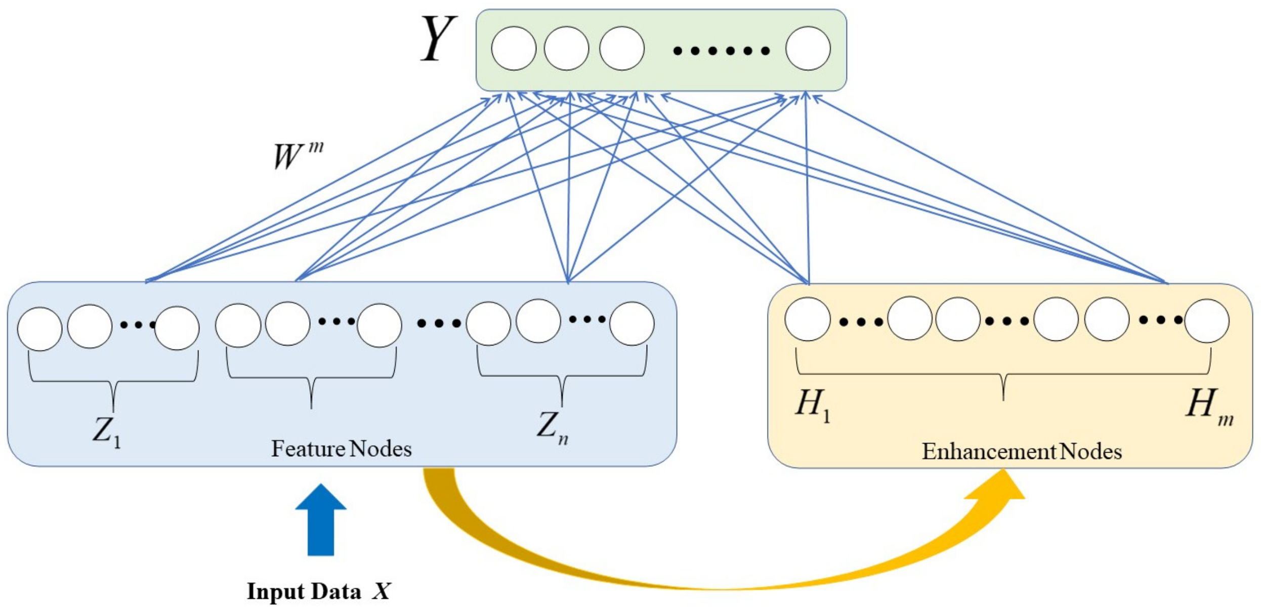
The structure of a basic BLS is improved on the basis of a random vector function linked neural network (RVFLNN), which eliminates the deep architecture and can realize efficient incremental learning. A BLS structure has fewer network layers compared with deep learning and is equipped with feature nodes and enhancement nodes. Of these, the feature nodes are mapped from the input data after feature extraction; the feature nodes are then multiplied by random weights plus random deviations and passed to the enhancement layer. The results of the feature layer and enhancement layer are ultimately combined and transferred to the output coefficient matrices, where the output weight is obtained via pseudo-inverse and ridge regression algorithms to avoid repeated calculation and to improve the efficacy of the modeling process. The basic structure and modeling process of a BLS are shown in Figure 2.
The given training dataset is { X L i , Y L i X L R B , Y L R C , i = 1 , 2 , , n } , where X L and Y L represent input data and output data with labels, respectively. After feature extraction, the input data generates mapping features to form n groups of feature nodes Z L i ( i = 1 , 2 , .. , n ) . The feature nodes Z L n of each group are represented as:
Z L i = ϕ i ( X L W z i + δ z i )
where Z L denotes the calculation result of the feature layer with labels and W z i denotes the weight coefficient, which is adjusted by applying a linear inverse problem to obtain the sparse representation of input data; δ z i denotes the bias coefficient and all are generated via random initialization. The transfer function is denoted by ϕ i ( ) , and Z L i = [ Z L 1 Z L i ] represents the feature nodes set.
The Z L n nodes are transformed via nonlinear activation function ξ j ( ) to finally generate m groups of enhancement nodes H L j ( j = 1 , , m ) .
H L j = ξ j ( Z L n W h j + δ h j )
In addition, H m [ H 1 , H 2 , , H m ] denotes the collection of all enhancement nodes. The output Y of a BLS is as follows:
Y L = [ Z L 1 , , Z L n | ξ ( Z L n W h 1 + δ h 1 ) , , ξ ( Z L n W h m + δ h m ) ] W e = [ Z L 1 , , Z L n , H L 1 , , H L n ] W e = [ Z L n , H L m ] W e
where W e denotes the weight of connecting the feature layer and enhancement layer to the output. W e could be easily calculated via the ridge regression approximation of pseudo-inverse.
If A = [ Z L n , H L m ] , W e can be obtained by the following objective function:
arg   min W e ( Y L Y L ^ 2 2 + λ 2 W e 2 2 )
where Y L Y L ^ 2 2 is used to control training error minimization. The purpose of this formula is to find the weight coefficient W e that minimizes the error between the predicted value and the true value; λ 2 W e 2 2 prevents overfitting, and λ denotes the regularization factor. The W e coefficient is then as follows:
W e = ( A T A + λ I ) 1 A T Y L
where I is the identity matrix, A T is the transpose matrix of A , and the pseudo-inverse of A can be expressed as:
A + = lim λ 0 ( A T A + λ I ) 1 A T
It follows that W e = A + Y L = [ Z L n , H L m ] + Y L .

2.3. Attention Mechanism

In complex machine-learning tasks, the attention mechanism is a common data processing method that can pay more attention to information that is more critical to the research object, solve the problem of information overload, reasonably allocate computing resources and improve the efficiency of task processing. The rolling bearing vibration of different signal segments has different contributions to the diagnosis results, and some features will interfere with the final results.
The SENet [18] attention module is introduced to measure various channel features in this paper. SENet mainly includes the key steps of squeeze and excitation. Squeeze refers to compressing the features of each channel as the descriptor of the channel and obtaining global channel features through the average pool. Excitation mainly captures the relationship between channels and generates the corresponding weight of each feature channel. The final step is reweight, after the feature selection of images, the output weight of excitation and the importance of each feature channel, weighted to the original feature information via multiplication to complete the recalibration in the channel dimension.

3. The Proposed SECNN–BLS Framework

A novel rolling bearing fault diagnosis method named SECNN–BLS was proposed, which first converts one-dimensional sample data points into multi-dimensional image inputs, then extracts fault feature information based on squeeze-and-excitation convolutional neural networks (SECNN) and uses the broad learning system (BLS) as the fault classifier; the final step is realizing the fault diagnosis on the machine fault prevention technology (MFPT) rolling bearing dataset. The overall construction of the framework is shown in Figure 3.
Figure 3a depicts the signal processing module, showing the process of converting the one-dimensional original vibration signal to the two-dimensional spectrum diagram, and Figure 3b shows the feature extraction module, which takes the stereoscopic two-dimensional spectrum diagram image as the input of CNN and adds the attention mechanism SENet to the CNN network structure to automatically acquire the importance of each channel of the image through learning, thus improving useful features and suppressing features that are not useful for the current task. Figure 3c shows the fault classification and recognition module. Here, BLS is used as a fault classifier to identify the fault.

3.1. Vibration Signal Processing

In the process of vibration signal processing, we use short-time Fourier transforms (STFT), which is actually a joint time–frequency analysis method mainly used to study non-stationary signal. It can describe the law of signal spectrum changing over time. The basic idea is to add a window to the signal (the window function will translate according to the change in time t ) and divide the signal into many small segments. If the signal on each segment can be regarded as stable, then the local signal on the small time segment near t at any time can be obtained, so that Fourier transform can be performed to form the two-dimensional time spectrum. The expression of the STFT of the continuous time signal s ( t ) is represented as follows:
S T F T ( t , ω ) = + [ s ( τ ) g ( τ t ) ] e j ω τ d τ
where S T F T ( t , ω ) is the two-dimensional complex function of time t and frequency ω , s ( τ ) is the original signal and g ( τ t ) is the window function. In signal processing, the STFT of the continuous-time signal s ( t ) in each window is generally replaced by the STFT of the discrete-time signal s ( n ) , so that the time and frequency are discrete, which is convenient for analysis and processing. The expression is as follows:
S T F T ( m , n ) = k = 0 L 1 s ( k ) g ( k m ) W L n k
where W L = e j 2 π / L , and L indicates the truncated signal length in the cycle.
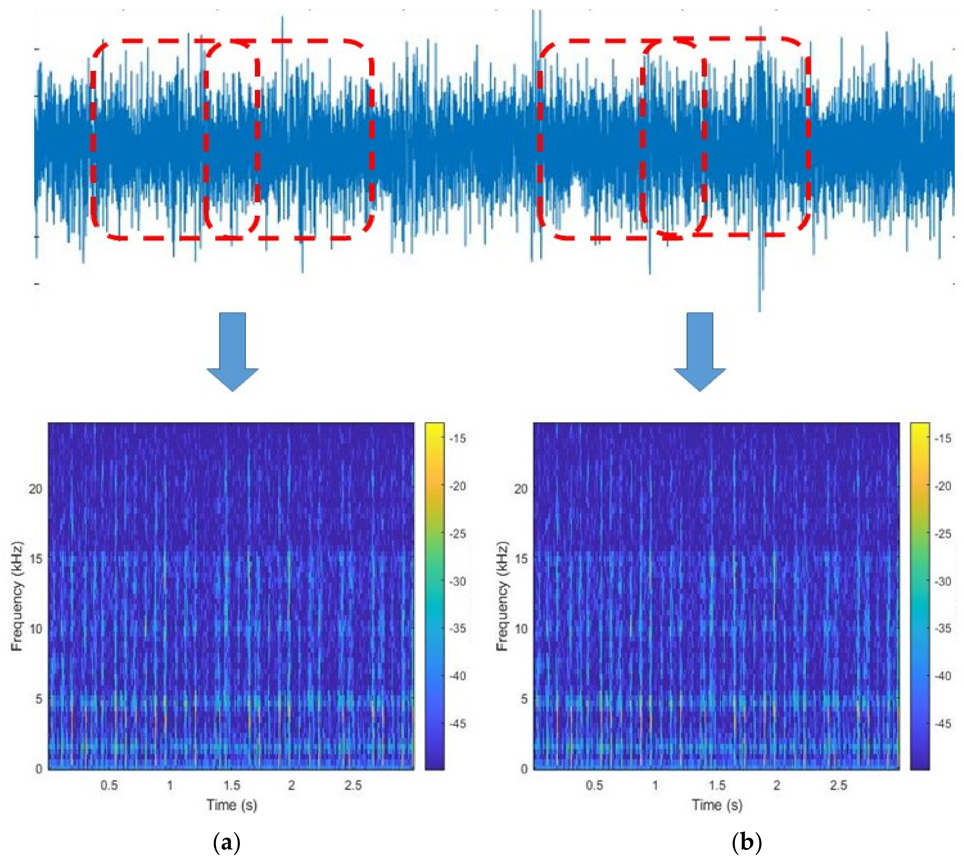
To obtain the information of a fault feature more intuitively and accurately, the real-time series signal of the rolling bearing in the dataset is first converted into the raw vibration signal in the time domain. The abscissa of the time domain analysis diagram is time, and the ordinate is the amplitude. The parameters are set according to the frequency of sampling and load of the rolling bearing data set; the overlapping sampling method of the sliding window is used to perform multiple STFTs [19] to draw the 2D spectrogram, as shown in the Figure 4, where Figure 4a,b show the two-dimensional spectrum of the one-dimensional vibration signal after STFT at different times. Figure 5 is a stereoscopic representation of the spectrogram as the input to SECNN–BLS, which can be drawn by Matlab 2020a to make the spectrum information from the signal more intuitive.

3.2. Feature Extraction Based on the SECNN

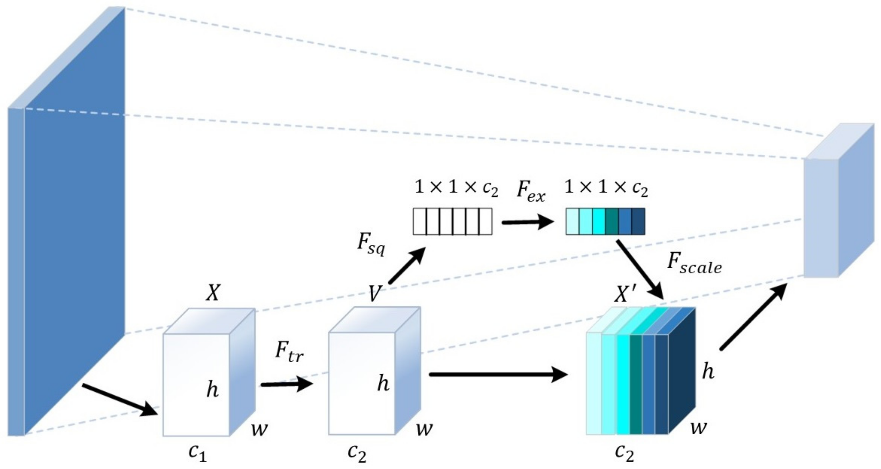
When the failure of the bearing emerges, the vibration signal data is not all abnormal, but only changes at some moments. Therefore, it is unnecessary to carry out the same learning process for each feature. It is essential to pay attention to some important features and eliminate interference from irrelevant feature information. To improve the efficiency of the feature extraction process, the squeeze-and-excitation networks (SENet) module is embedded in the structure of the CNN. As a lightweight structure, SENet has good embeddedness. Without increasing the time and space complexity, SENet is embedded in the CNN structure to replace the convolution layer for feature information extraction, which can expand from the local receptive field to global information extraction and recalibrate the image channel information. First, through the squeezing operation, a global descriptor is generated across the spatial dimension. This global descriptor aggregates the spatial information from all channels, and then the excitation operation is performed to capture the importance of image channels and to control the excitation of each channel. The feature map is then reweighted to generate the output of the SENet block and combined with the previous block to extract the channel association information. The construction process is illustrated in Figure 6.
Different colors represent different weights. The main principle is to introduce the attention mechanism on the channel dimension in the CNN convolution process. For the feature map X with the given dimension c 1 × w × h , the feature map V with the dimension c 2 × w × h is obtained after an ordinary convolution transformation. After the squeeze operation, compressing with the spatial dimension of w × h , the output after squeeze operation u c is obtained via the following formula:
u c = F s q ( V c ) = i = 1 w j = 1 h V c ( i , j ) w × h
F s q represents the squeeze function, which corresponds to a global average pooling operation. Following compression of a characteristic graph of c × w × h into c × 1 × 1 , the results obtained can represent global information. Through the excitation operation, different weights are assigned to the c 2 channels according to the importance of each channel The corresponding expression is as follows:
z = F e x ( u , W ) = σ ( W 2 δ ( W 1 u ) )
where F e x denotes the excitation function. The corresponding channel weights are obtained through two full connection operations and activation functions, where W 1 is the dimension reduction parameter of the first full connection operation, W 2 is the restoration dimension parameter of the second full connection, σ is the sigmoid function for weight normalization and δ is the ReLU function.
X c = F s c a l e ( V c , z c ) = z c V c
Finally, the output weight matrix z and the input feature map V are multiplied by the F s c a l e function, which can reweight feature maps to obtain the input high-level feature X c of the next layer structure, which is expressed as Equation (12).

3.3. Fault Diagnosis Based on the SECNN–BLS

This paper considered combining the SECNN feature extraction module with the BLS fault classification module. As presented in the Figure 2, through the convolution, attention mechanism fusion and maximum pooling operations of the input image, the output of the last convolutional layer or pooling layer is retained as the extracted image features mapped to the feature nodes of BLS. The main steps of the SECNN–BLS method are summarized as follows:
Step 1: Divide the vibration signal of the rolling bearings into multiple sections, set the length of the window to 4000 and the length of overlap to 2000, convert the time series vibration signal to the frequency spectrum in the time-frequency domain through STFT, set labels for the samples, divide these into training sets and test sets according to a ratio of 2:1.
Step 2: Load the pre-trained SECNN network, input the preprocessed samples in step 1 into the model and set the convolution core size to 3 × 3 and the length of stride to 2; the activation function uses ReLu for the convolution operation.
Step 3: Input the feature maps obtained after the convolution calculation into the SENet module, calculate the importance of different channels of the feature maps and assign corresponding weights; next, pass the channel feature map multiplied by the weights to the global maximum pooling layer.
Step 4: The high-level feature representation of the image obtained from the pooling layer is used as the BLS input and mapped into feature nodes; enhanced nodes are generated through nonlinear functions to form an augmented matrix to train the fault classifier. Finally, test samples are used to verify the validity of the fault diagnosis model.

4. Experiment

The SECNN–BLS method was applied to the MFPT rolling bearings dataset to verify its performance compared with several integrated deep-learning methods including the following: multisynchrosqueezing transform and sparse feature coding based on dictionary learning (MSST+SFC-DL) [20], refined composite multiscale fluctuation-based dispersion Lempel–Ziv complexity (RCMFDLZC) [21] and typical deep-learning methods, including traditional CNN [22], stacked autoencoder (SAE) and several other improved methods based on CNN. These included residual net (ResNet), attention mechanism residual network (A-ResNet) and continuous wavelet transform ResNet (CWT-ResNet) [23]. The experimental results show that the proposed method has the highest detection accuracy in both normal and noisy environments compared with other methods.

4.1. Data Description

The MFPT dataset includes vibration signals collected from rolling bearings under 23 different health condition categories: three types of rolling bearing data under normal conditions at constant load, three types of outer race fault data under constant load, seven categories of outer race faults and seven categories of inner race faults under different loads. In addition, there are three types of bearing data with unknown fault locations collected from real-world scenarios. In this paper, 20 categories of labeled data samples in the MFPT dataset are used to verify the effectiveness of the model. The specific parameters are listed in Table 1.
Due to the large number of data points, the sliding window method was adopted for overlapping sampling. The length of the window was set to 4000, and the length of the overlap was 2000, i.e., each sample contained 4000 sampling data points. The sample size under each state of the final rolling bearing is shown in Table 1. The sample size under each label was divided into a training set and a test set at a ratio of 2:1.

4.2. Analysis of Experimental Results

When evaluating the performance of the SECNN–BLS fault diagnosis method for each type of fault, there are four categories of indicators as follows: Accuracy, Precision, Recall and F1-Score.
F 1 - Score = 2 × Precision × Recall Precision + Recall
In addition, observing two indicators simultaneously has more reference value; here we have selected a frequently used measurement curve and calculated the area under the curve (AU). We used the receiver operator characteristic (ROC) curve, which plots the false positive rate (FPR) versus the true positive rate (TPR).
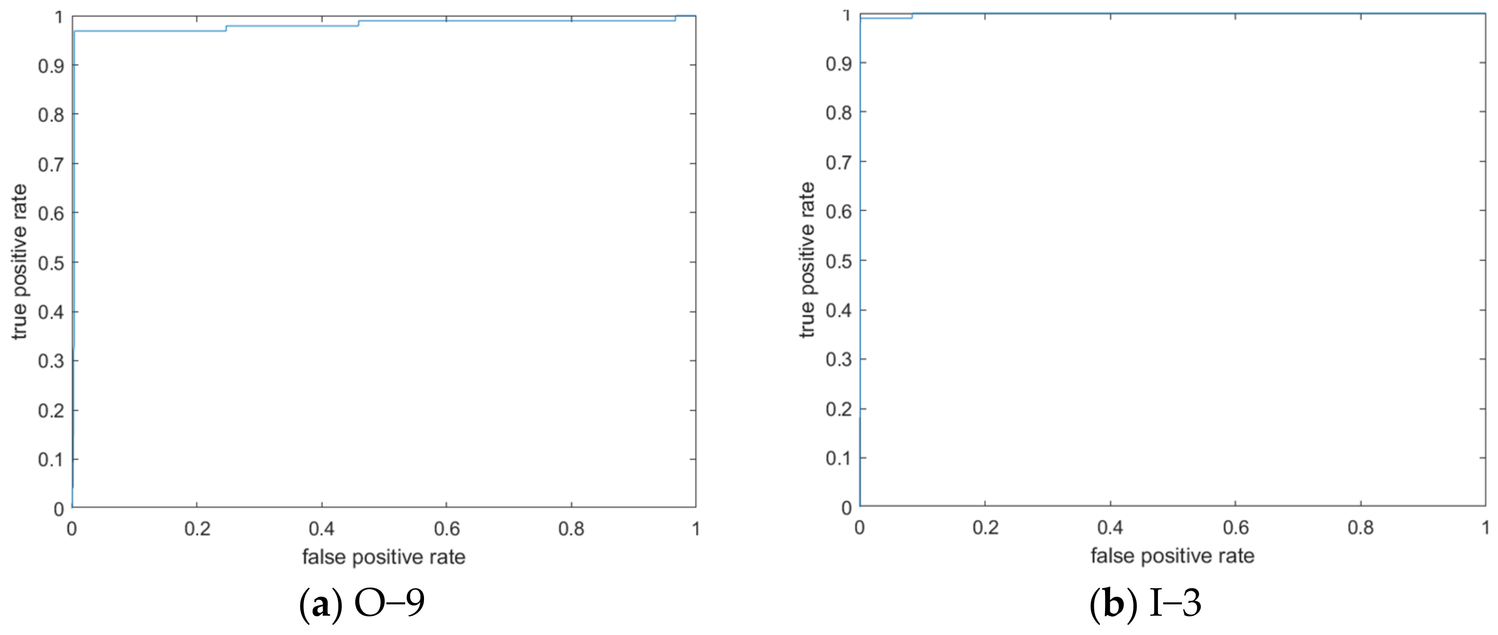
The results in Table 2 prove that among the 17 types of inner and outer race faults, the classification accuracy of SECNN–BLS is above 96%, with most reaching 98%. In the O-1, O-4, O-9, I-1 and I-3 fault categories, the accuracy rate reaches 99%. The AU-ROC values are around 95%, indicating that the fault diagnosis model is feasible and effective. Table 3 illustrates that SECNN–BLS has achieved the highest diagnostic accuracy of 98.31% compared to the other methods.
Figure 7 depicts the ROC curves for the categories with the highest diagnostic accuracy, shown separately in terms of the outer race fault and inner race fault. It is obvious that the curves are close to the upper left corner, which indicates that the larger the area below the curves, the better the performance of the method.

4.3. Performance under Additional Noise Conditions

This section mainly evaluates the anti-interference ability of SECNN–BLS in a noisy environment. In the actual industrial production environment, noise pollution is inevitable in the collected vibration signal data of rolling bearings; this will interfere with the detection and identification of faults and affect the accuracy of fault diagnosis. In order to verify the robustness and stability of the model, we introduced Gaussian white noise into the original vibration signal. The signal-to-interference plus noise ratio (SNR) is expressed as follows:
SNR = 10 log 10 P s P n
where P s and P n represent the effective power of the vibration signal and the added Gaussian white noise, respectively; the unit of SNR is dB. The Gaussian white noise range used in this paper is −4 dB~12 dB.
Five fault diagnosis methods were selected to compare with this method, including a stacked autoencoder network (SAE), a CNN and several other improved methods based on CNN: residual net (ResNet), attention mechanism residual network (ARes–Net) and continuous wavelet transform ResNet (CWT–ResNet). The specific results of the experiment are shown in Table 4. It is obvious that noise will have a certain impact on the accuracy of fault diagnosis, but with the gradual increase in SNR, the accuracy rate will be significantly improved. Compared with the other five methods, SECNN–BLS has the highest diagnostic accuracy in a noisy environment. When SNR = −4 dB, it can still maintain more than 80% accuracy, and when SNR = 12 dB, the accuracy of the fault diagnosis can reach 98.21%. Figure 8 is a visual representation of the experimental results with a broken line diagram, which shows consistently superior performance for SECNN–BLS.

5. Conclusions

In this paper, a novel method named SECNN–BLS is proposed. Through multiple discrete STFTs, a one-dimensional rolling bearing vibration signal is initially transformed into a two-dimensional spectrogram as the CNN input, which maximally retains the original features. We then introduced an attention mechanism into the feature extraction process by replacing the convolution layers with SENet modules, adaptively assigning weights according to the importance of image channel information. This, in turn, improves the contribution degree of important information, eliminating interference from irrelevant features. Introducing a BLS in the failure classification stage effectively increases the fault classification accuracy. The final experimental results show that the performance of the proposed method is superior, while still maintaining high diagnostic accuracy in noisy environments, making it better adapted to complex industrial environments.
Although corresponding solutions have been proposed for the problem of more efficient deep feature extraction and fault classification, there are still some problems worthy of in-depth study, such as how to improve the applicability of the model and be able to deal with the modeling problem of changeable working conditions and nonstationary data. In addition, due to space limitations, research on BLS incremental learning has not yet been conducted, which will be a direction for future work.

Author Contributions

Conceptualization, X.W.; writing, manuscript preparation, T.H.; review and editing, S.X.; supervision and project management, X.Z. All authors have read and agreed to the published version of the manuscript.

Funding

This research was supported by the National Natural Science Foundation of China grant Nos. U2001201 and 61876055.

Data Availability Statement

The data of this paper came from the Society for Machinery Failure Prevention Technology (MFPT), and the data acquisition website used was https://www.mfpt.org/fault-data-sets/, accessed on 10 June 2022.

Conflicts of Interest

The authors declare no conflict of interest.

References

  1. Wang, G.; Hu, Z. Bearing fault diagnosis based on multi-scale mean permutation entropy and parametric optimization SVM. J. Vib. Shock. 2022, 41, 221–228. [Google Scholar]
  2. Zhang, J.; Wu, J.; Hu, B. Intelligent fault diagnosis of rolling bearings using variational mode decomposition and self-organizing feature map. J. Vib. Control. 2020, 26, 1886–1897. [Google Scholar] [CrossRef]
  3. Tang, S.; He, J.; Ren, J. Research on fault diagnosis of rolling bearing based on the improved EWT method of spectral envelope. Renew. Energy 2022, 40, 825. [Google Scholar] [CrossRef]
  4. Wang, D.; Zhao, Y.; Yi, C. Sparsity guided empirical wavelet transform for fault diagnosis of rolling element bearings. Mech. Syst. Signal Process. 2018, 101, 292–308. [Google Scholar] [CrossRef]
  5. Guo, T.; Deng, Z. An improved EMD method based on the multi-objective optimization and its application to fault feature extraction of rolling bearing. Appl. Acoust. 2017, 127, 46–62. [Google Scholar] [CrossRef]
  6. Wang, L.; Liu, Z.; Miao, Q. Complete ensemble local mean decomposition with adaptive noise and its application to fault diagnosis for rolling bearings. Mech. Syst. Signal Process. 2018, 106, 24–39. [Google Scholar] [CrossRef]
  7. Wang, Z.; Zhang, Q.; Xiong, J.; Xiao, M.; Sun, G.; He, J. Fault Diagnosis of a Rolling Bearing Using Wavelet Packet Denoising and Random Forests. IEEE Sens. J. 2017, 17, 5581–5588. [Google Scholar] [CrossRef]
  8. Guo, S.; Zhang, B.; Yang, T.; Yu, D.; Gao, W. Multitask Convolutional Neural Network with Information Fusion for Bearing Fault Diagnosis and Localization. IEEE Trans. Ind. Electron. 2020, 67, 8005–8015. [Google Scholar] [CrossRef]
  9. Gao, S.; Shi, S.; Zhang, Y. Rolling Bearing Compound Fault Diagnosis Based on Parameter Optimization MCKD and Convolutional Neural Network. IEEE Trans. Instrum. Meas. 2022, 71, 1–8. [Google Scholar] [CrossRef]
  10. Wang, H.; Liu, Z.; Peng, D.; Qin, Y. Understanding and Learning Discriminant Features based on Multiattention 1DCNN for Wheelset Bearing Fault Diagnosis. IEEE Trans. Ind. Inform. 2020, 16, 5735–5745. [Google Scholar] [CrossRef]
  11. Xu, Z.; Li, C.; Yang, Y. Fault diagnosis of rolling bearings using an Improved Multi-Scale Convolutional Neural Network with Feature Attention mechanism. ISA Trans. 2021, 110, 379–393. [Google Scholar] [CrossRef]
  12. Chen, L.P.; Liu, Z.L. Broad learning system: An effective and efficient incremental learning system without the need for deep architecture. IEEE Trans. Neural Netw. Learn. Syst. 2018, 29, 10–24. [Google Scholar] [CrossRef] [PubMed]
  13. Xu, M.; Han, M.; Chen, L.P.; Qiu, T. Recurrent Broad Learning Systems for Time Series Prediction. IEEE Trans. Cybern. 2020, 50, 1405–1417. [Google Scholar] [CrossRef]
  14. Yu, W.K.; Zhao, C.H. Broad Convolutional Neural Network Based Industrial Process Fault Diagnosis with Incremental Learning Capability. IEEE Trans. Ind. Electron. 2020, 67, 5081–5091. [Google Scholar] [CrossRef]
  15. Chen, L.P.; Liu, Z.L.; Feng, S. Universal Approximation Capability of Broad Learning System and Its Structural Variations. IEEE Trans. Neural Netw. Learn. Syst. 2019, 30, 1191–1204. [Google Scholar] [CrossRef] [PubMed]
  16. Fu, Y.; Cao, H.; Chen, X. Adaptive Broad Learning System for High-Efficiency Fault Diagnosis of Rotating Machinery. IEEE Trans. Instrum. Meas. 2021, 70, 1–11. [Google Scholar] [CrossRef]
  17. Cheng, C.; Wang, W.J.; Chen, H.T.; Zhang, B.C.; Shao, J.J.; Teng, W.X. Enhanced Fault Diagnosis Using Broad Learning for Traction Systems in High-Speed Trains. IEEE Trans. Power Electron. 2021, 36, 7461–7469. [Google Scholar] [CrossRef]
  18. Hu, J.; Shen, L.; Sun, G. Squeeze-and-excitation networks. In Proceedings of the 2018 IEEE CVF Conference on Computer Vision and Pattern Recognition, Salt Lake City, UT, USA, 18–22 June 2018; pp. 7132–7141. [Google Scholar] [CrossRef]
  19. Yu, S.-S.; Zhou, N.-R.; Gong, L.-H.; Nie, Z. Optical image encryption algorithm based on phase-truncated short-time fractional Fourier transform and hyper-chaotic system. Opt. Lasers Eng. 2020, 124, 105816. [Google Scholar] [CrossRef]
  20. Sun, G.; Gao, Y.; Lin, K.; Hu, Y. Fine-grained fault diagnosis method of rolling bearing combining multisynchrosqueezing transform and sparse feature coding based on dictionary learning. Shock. Vib. 2019, 2019, 1531079. [Google Scholar] [CrossRef]
  21. Li, Y.; Jiao, S.; Geng, B. Refined composite multiscale fluctuation-based dispersion Lempel–Ziv complexity for signal analysis. ISA Trans. 2022, in press. [Google Scholar] [CrossRef]
  22. Verstraete, D.; Ferrada, A.; Lopez Droguett, E.; Meruane, V.; Modarres, M. Deep learning enabled fault diagnosis using time-frequency image analysis of rolling element bearings. Shock Vib. 2017, 2017, 5067651. [Google Scholar] [CrossRef]
  23. Wang, Y.; Liang, J.; Gu, X.; Ling, D.; Yu, H. Multi-scale attention mechanism residual neural network for fault diagnosis of rolling bearings. Proc. Inst. Mech. Eng. 2022, 236, 10615–10629. [Google Scholar] [CrossRef]
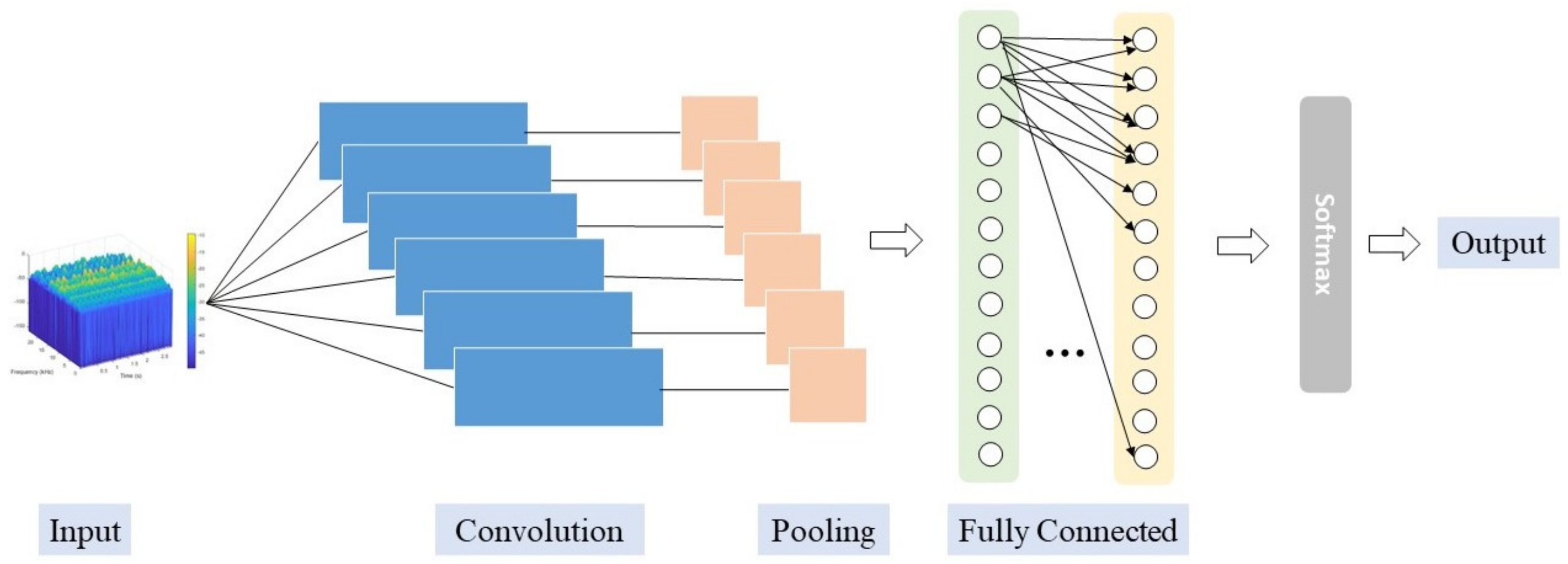
Figure 1. Framework of a convolutional neural network (CNN).
Machines 11 00279 g001
Figure 2. Framework of a typical BLS.
Machines 11 00279 g002
Figure 3. Framework of SECNN−BLS.
Machines 11 00279 g003
Figure 4. Conversion from vibration signal to time–frequency domain image.
Machines 11 00279 g004
Figure 5. Input image of SECNN–BLS ((a) is the image of the baseline rolling bearing, (b) is the inner race fault, and (c) is the outer race fault).
Machines 11 00279 g005
Figure 6. The realization process of the SENet attention mechanism.
Machines 11 00279 g006
Figure 7. ROC curves for the fault diagnosis for the inner ring and outer ring ((a) is the ROC curve of label O-9, and (b) is the ROC curve of label I-3).
Machines 11 00279 g007
Figure 8. Comparison results of different methods in different noise environments.
Machines 11 00279 g008
Table 1. The parameters of MPFT dataset.
Fault ConditionLabelLoad (lbs)Input Shaft Rate (Hz)Sample Rate (sps)Time (s)Number of Data PointsNumber of Training SamplesNumber of Testing Samples
BaselineB-1, B-2, B-32702597,6566585,93619497
Outer Race FaultO-1, O-2, O-32702597,6566585,936534267
O-4, O-5, O-6, O-7, O-8, O-9, O-1025, 50, 100, 150, 200, 250, 3002548,8283146,484 × 7
Inner Race FaultI-1, I-2, I-3, I-4, I-5, I-6, I-70, 50, 100, 150, 200, 250, 3002548,8283146,484 × 7340170
Table 2. Performance metrics for each type rolling bearing fault.
LabelPrecisionRecallF1-ScoreAU-ROCAccuracy
O-199.74%90.65%94.98%95.50%99.74%
O-296.51%97.66%97.08%95.15%96.51%
O-397.17%97.43%97.30%95.15%97.17%
O-499.92%94.21%96.98%95.30%99.92%
O-597.90%93.39%95.59%95.35%97.90%
O-698.94%95.60%97.24%95.25%98.94%
O-797.17%97.50%97.34%95.15%97.17%
O-896.20%96.13%96.17%95.20%96.20%
O-999.88%93.49%96.58%95.35%99.88%
O-1098.10%97.04%97.57%95.15%98.10%
I-199.97%96.65%98.28%95.20%99.97%
I-298.17%97.67%97.92%95.15%98.17%
I-399.99%98.85%99.42%95.10%99.99%
I-496.62%95.22%95.92%95.25%96.62%
I-597.26%97.86%97.56%95.15%97.26%
I-698.95%94.24%96.54%95.30%98.95%
I-798.79%91.33%94.92%95.45%98.79%
Table 3. Results of fault diagnosis accuracy compared with other methods on the MFPT dataset.
LiteratureFeature ExtractionFault IdentificationFault TypesAverage Accuracy (%)
[20]MSST+SFC-DLLSVM395.83
[21]RCMFDLZCDAC396.05
[22]CNNHHT392.90
[23]SAESoftmax390.11
[23]CNNFully Connected Layer, Softmax394.33
[23]ResNetFully Connected Layer, Softmax396.83
[23]Attention Mechanism
ResNet
Fully Connected Layer, Softmax397.87
This paperSECNNBLS398.31
Table 4. Comparison results of fault diagnosis accuracy under a noisy environment with other methods on the MFPT dataset.
MethodAccuracy (%) under Different SNR (dB)
−404812
SAE55.3969.3281.2287.3389.27
CNN61.5777.1383.8991.2592.95
ResNet64.4480.4989.7394.8496.03
A−ResNet75.0586.5492.8696.4797.52
CWT−ResNet72.8685.0792.4796.2898.06
SECNN–BLS81.2292.0895.7697.8398.21
Disclaimer/Publisher’s Note: The statements, opinions and data contained in all publications are solely those of the individual author(s) and contributor(s) and not of MDPI and/or the editor(s). MDPI and/or the editor(s) disclaim responsibility for any injury to people or property resulting from any ideas, methods, instructions or products referred to in the content.