Hybrid Analytical Modeling of Force Dense Segmented Magnetic Linear Actuator with Non-Dimensional Parametric Modeling of the Magnetic Flux Effects

Abstract

A new advanced two-dimensional hybrid analytical model of a segmented magnet linear actuator (MLA) comprised of surface permanent magnets (PM) is developed in this paper. This model is used to predict and evaluate the performance of the segmented MLA with proper correction on magnetic Flux Effects, validated by computational modeling. An MLA design with non-uniform PM segmentation was applied in this research to improve its performance compared with conventional radially magnetized MLA and uniform segmented Halbach Array based MLA. For MLA thrust force prediction, the previous published analytical model does not consider losses due to two observed magnetic Flux Effects: (1) the magnetic edge effect—the diminishing nature of the magnetic flux at the edge of the MLA, and (2) the observed magnetic interaction effect—the inconsistent peaks of individual magnetic flux lines, lower than the overall peak flux. In the proposed hybrid model for the segmented MLA, the shaft magnetic field distribution is based on a scalar potential theory subdomain method and the ring magnetic field is based on equivalent surface distributed currents. Collectively, these models are combined with three-dimensional finite element analysis (FEA), to estimate the magnetic thrust force. A data driven pole correction factor is introduced, based on the FEA computational database of three-dimensional MLA, to capture the losses associated with the magnetic flux, which is not considered in the analytical subdomain method. Finally, a normalized pole correction is proposed to generalize the model to different magnetic grades, different dimensional constraints, and varying magnet ratios of the segmented magnets. The developed model provides the design basis for manufacturing optimized force dense segmented MLAs for rotary to linear actuation, based on the force required for the application without the need for running FEA analysis after each design iteration, reducing costs and time required for the optimal design.

1. Introduction

A linear actuator is a device that converts rotary motion to linear. Applications demanding high force, precision, and high-speed performance are met by utilizing devices such as tubular linear actuators. Linear actuators are used in various industrial machinery, machine tools, valves, dampers, and computer hardware. Magnetic Linear Actuators, or MLAs, are devices where the mechanical power transmission is replaced by a magnetic arrangement which actuates the mechanism. MLAs have a broad range of applications including offshore oil and gas production, transportation, manufacturing, automation, aerospace, military, and healthcare systems. The primary benefit of MLAs includes clean, oil-free operation, high force densities, lag-free operation, and high reliability [1,2,3]. MLAs minimize fatigue loading while creating minimal noise generation during operation. Additional MLA applications are presented in [4] where the linear drives control the motion of a load directly, and passive magnetic bearings and magnetic couplings support the flywheel rim. MLAs have also been recently proposed for wave energy harvesting [5,6].

MLAs emerged as a provider of high-density force when the replacement of conventional magnet arrangements with Halbach Array was explored [3,7,8,9,10,11,12]. The Halbach Array is a spatially rotating pattern of permanent magnets that augments the magnetic field on one side of the array while almost nullifying the field on the opposite side. Wang et al. [10] devised a general framework for high density linear electromagnetic actuators, presenting the design of tubular linear magnetic machines. This work led to investigations focusing on smaller embodiments used for applications, such as in artificial heart devices [3,7,10]. The concept was adapted for linear actuators comprised of a ring and shaft embodiment where the magnetic arrangement was helically wound around the shaft and on the inner side of the ring structure [5]. Considering the magnetic field interactions between a magnetic ring and a magnetic shaft along with the thrust force generated within the system, these studies employed Halbach Array designs [2,3,8,10,12,13,14,15], deviating from the radially magnetized permanent magnet-based work of Wang et al. [7]. The analytical modeling studies used equivalent current based approaches to calculate the thrust force due to the magnetic interactions in the ring and shaft framework [7,10].

Conventional radial MLAs have been modeled in [5,7,8,9,15]. The present paper presents an advancement to that knowledgebase by using segmented magnets instead of conventional magnets, which focuses the magnetic flux in the active working region (the airgap) and reduces flux in the inactive passive region (the back iron). Physics-based models of linear actuators consisting of segmented permanent magnets are developed in this study which are superior to conventional radially oriented magnets in terms of producing higher flux density in the active region, thereby producing higher thrust force [2,3,4,12,16,17]. This high force segmented MLA has potential application in artificial heart technology [3,15], with remarkable servo characteristics, absence of static fatigue loading, and frictionless and noise-free mechanism. Segmented MLAs produce high force density based on a ring and shaft framework, using magnetic coupling to convert rotary motion into linear motion by direct linear magnetic-mechanical energy conversion [6]. The segmenting of the magnets, called the Halbach Array when the segments are uniformly sized, configures a high thrust force linear actuator, which has a stronger magnetic flux concentration towards the air gap region [13,16,18]. The sinusoidal behavior of the magnetic flux makes it a well-controlled device with reliable servo characteristics [4,19] and dynamic performance, and the fewer magnetic losses increase workability and applicability of the system.

A subdomain model for the segmented magnetic arrangement is developed in the present work based on scalar potential theory [20]. Analytical models for predicting the magnetic field for rectangular permanent magnets, which was based on conventional magnets, led the way to modeling segmented magnetic arrangements by breaking down the magnetic field due to the Halbach array arrangement into the axial and radial components [7,10,17,21,22]. The segmented magnetic arrangement on the ring is represented as equivalent surface distributed currents [10,17,22] for the development of the magnetic thrust force model for a single pole, which consists of a radially magnetized segment and an axially magnetized segment. With the interactions of the magnetic field produced by the magnets on the shaft and the equivalent surface distributed currents, the thrust force on the ring is calculated using a surface integration of the cross product of the surface current density and the respective magnetic field [5,7,10,17].

Previous analytical models based on conventional magnets have been presented for small dimensional applications by calculating the thrust force acting on a single pole of magnets on the shaft. Then, the system thrust force would be calculated by multiplying the single-pole force by the number of the active poles in this ring and shaft system. However, upon thorough investigation of the same embodiment at different sizes, magnetic losses, such as edge losses, were found. This was due to the gradual mitigations of magnetic flux on both ends of the shaft, which were not negligible when the dimensions of the ring and shaft were larger than the small dimensional applications such as in [3,7]. An interaction effect of the magnetic flux was also observed, where the magnetic flux magnitude was not consistent for all the poles. Thus, without accounting for such edge losses, previously published works and analytical models could potentially over-estimate the thrust force provided by the MLA, especially for larger dimensional applications with same number of magnet poles, where the interaction effect is also significant. Therefore, it will be necessary to correct and re-calibrate the thrust force calculation of the MLA, considering such losses. In the presented study, it was found that these losses are proportional to the ratios of dimensions such as air gap over lead length, lead over magnet thickness, etc. These losses result in a decrease in magnetic flux density and, therefore, the thrust force, due to the magnetic poles at the edges and the magnetic flux interaction losses in the magnetic poles away from the edges. These losses were modelled by utilizing the FEA results as a database, fitting the losses into one model and combining with the subdomain model to estimate the thrust force for which the detailed study is presented in the further sections. To account for multiple active poles, an original pole correction factor is introduced in the present work. The normalized pole correction factor is then derived as a multiplicative variable to better understand the implementation of this model. This also accounts for the magnetic losses and for the variations in the magnet ratio of the segmented magnet arrangement. The mathematical model is validated using finite element analysis in Ansys electronics desktop 2020R2, and the results of Ji et al. [3] were compared for validation.

Section 2 of the paper presents the mathematical models and the derived equations. It includes the derivation for the magnetic flux density for the segmented magnetic arrangement and the thrust force calculation using the equivalent current based approach for the magnetic interactions on the ring and shaft framework. Section 3 presents the development of the pole correction factor, modeling for the edge losses and interaction losses, and Section 4 presents the results based on the derived models and validation with FEA results on a set of design parameters. Section 5 is the conclusion of the paper.

2. Magnetic Linear Actuator Model

In this section, a model structure is developed that generalizes the embodiment of an MLA for modeling purposes. The ring-shaft embodiment (Figure 1) of the MLA has three primary subdomains: (I) the airgap, (II) the magnets, and (III) the back-iron. The analytical model developed in this study is used for estimating the magnetic flux densities in these different regions, thus, enabling thrust force calculations generated by the magnetic interaction between the ring and shaft. The magnetic flux density of the shaft surface permanent magnets is modeled using scalar potential theory. Subsequently, the magnetic flux densities for the ring are modeled using equivalent surface distributed currents. Collectively, these estimated flux densities are used to calculate the magnetic field in Region I (the airgap) to later estimate the thrust force.

2.1. System Configuration

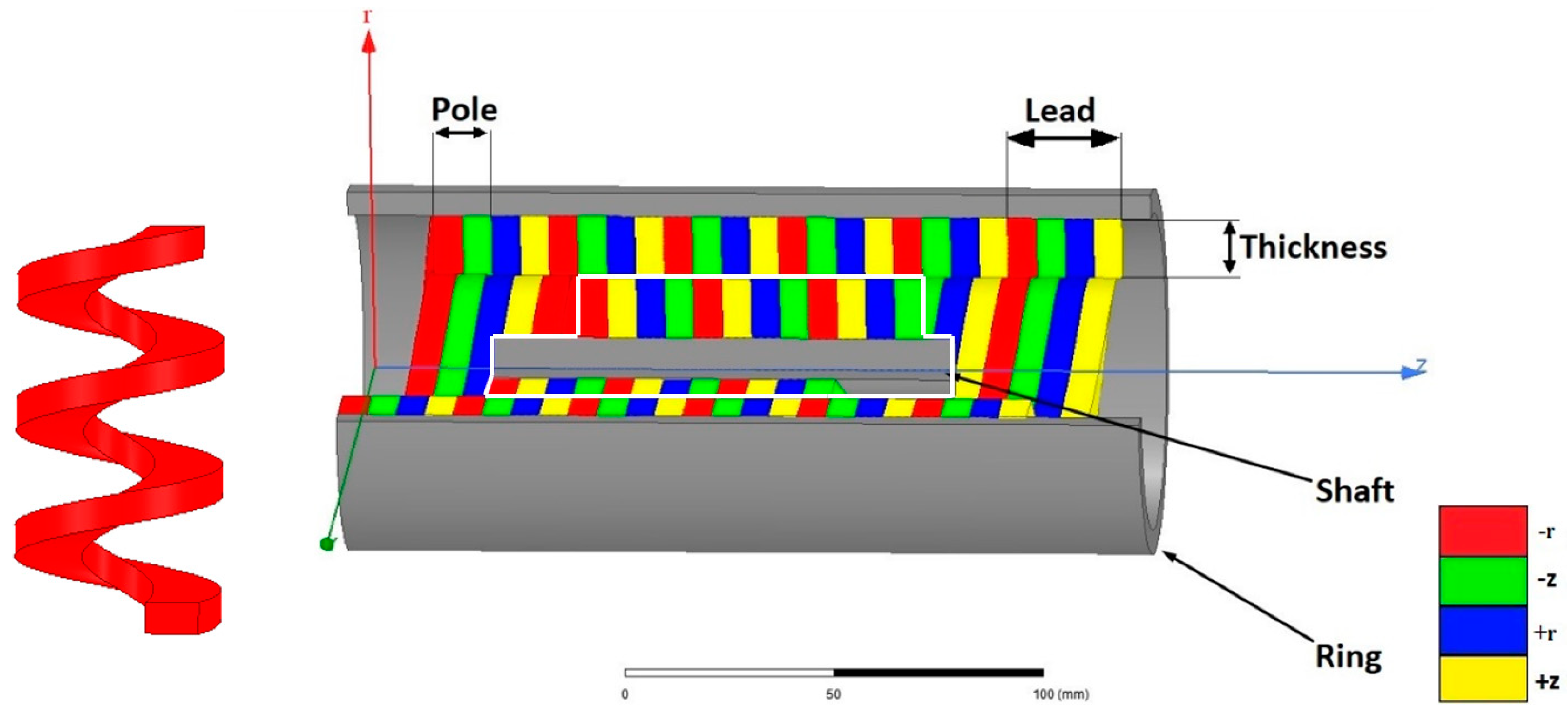
The MLA embodiment presented in Figure 1 consists of a ring and a shaft framework. Both the ring and the shaft have a spatially rotating pattern of magnetic flux, resulting from the magnetic arrangements that are helically mounted on the surface [3,5,7,15].

The MLA thrust force developed is due to the displacement of the magnetic shaft relative to the magnetic ring. The maximum thrust force develops when the relative displacement between the ring and the shaft magnets is$\left(2n-1\right)\frac{\tau }{2}$ where $\tau$ is the length of one pole, denoted as pole pitch, and $n\in Z_{+}$.

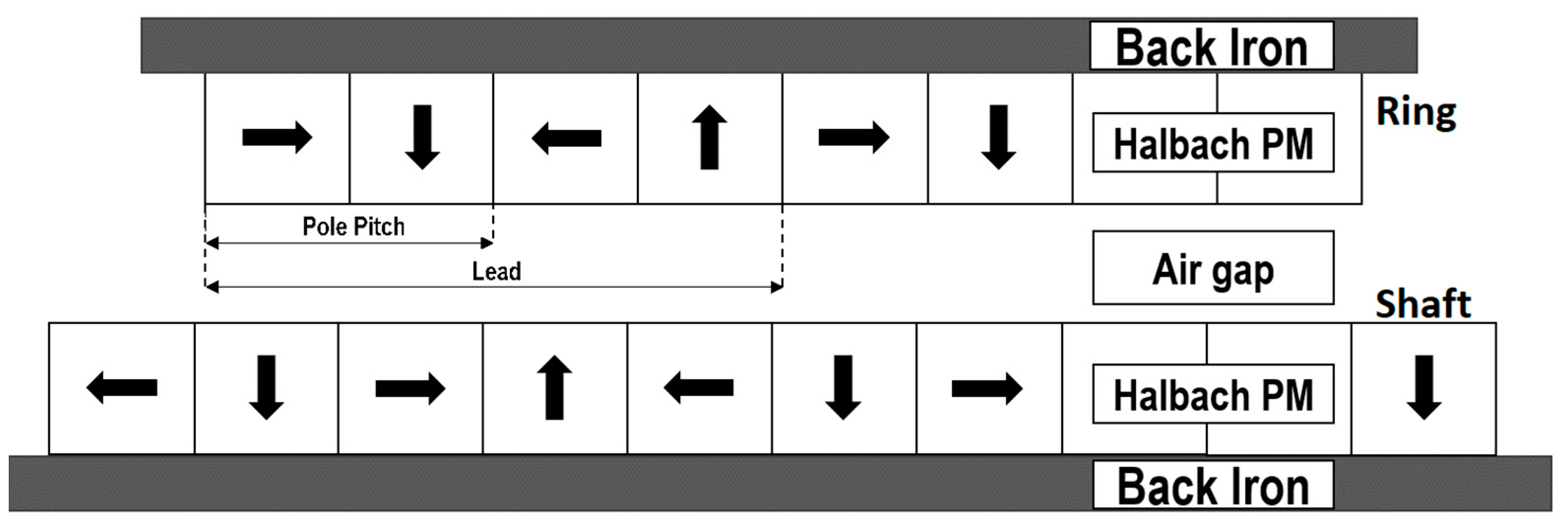
A two-dimensional representation of an MLA cross-section is shown in Figure 1 and the three-dimensional representation is provided in Figure 2.

The shaft and ring configuration, both having helical permanent magnets, are the two components of this system. The permanent magnets are arranged in accordance with the segmented magnetic configuration, the main advantage of which is the enhancement of the magnetic field interactions between shaft and the ring subsystems in the air gap region [3,7,15]. A general segmented magnetic arrangement consists of four magnetic segments, with the alternate piece magnetization rotated by 90° about the vector tangent to the shaft, within an axial distance of the lead $\lambda$ (equal to $2\tau$).

The magnet ratio, $M_R$, is the ratio of axial direction length of the radially magnetized permanent magnet, ${\tau }_r$, to the pole length, $\tau$.

$$M_R=\frac{{\tau }_r}{\tau }$$

(1)

The individual segments in Figure 1 have the same axial width, and two such segments together form a pole. With a magnet ratio of 0.5, this segmented magnet case reduces to the Halbach array. In the present work, this generalization of the magnet ratio will be considered.

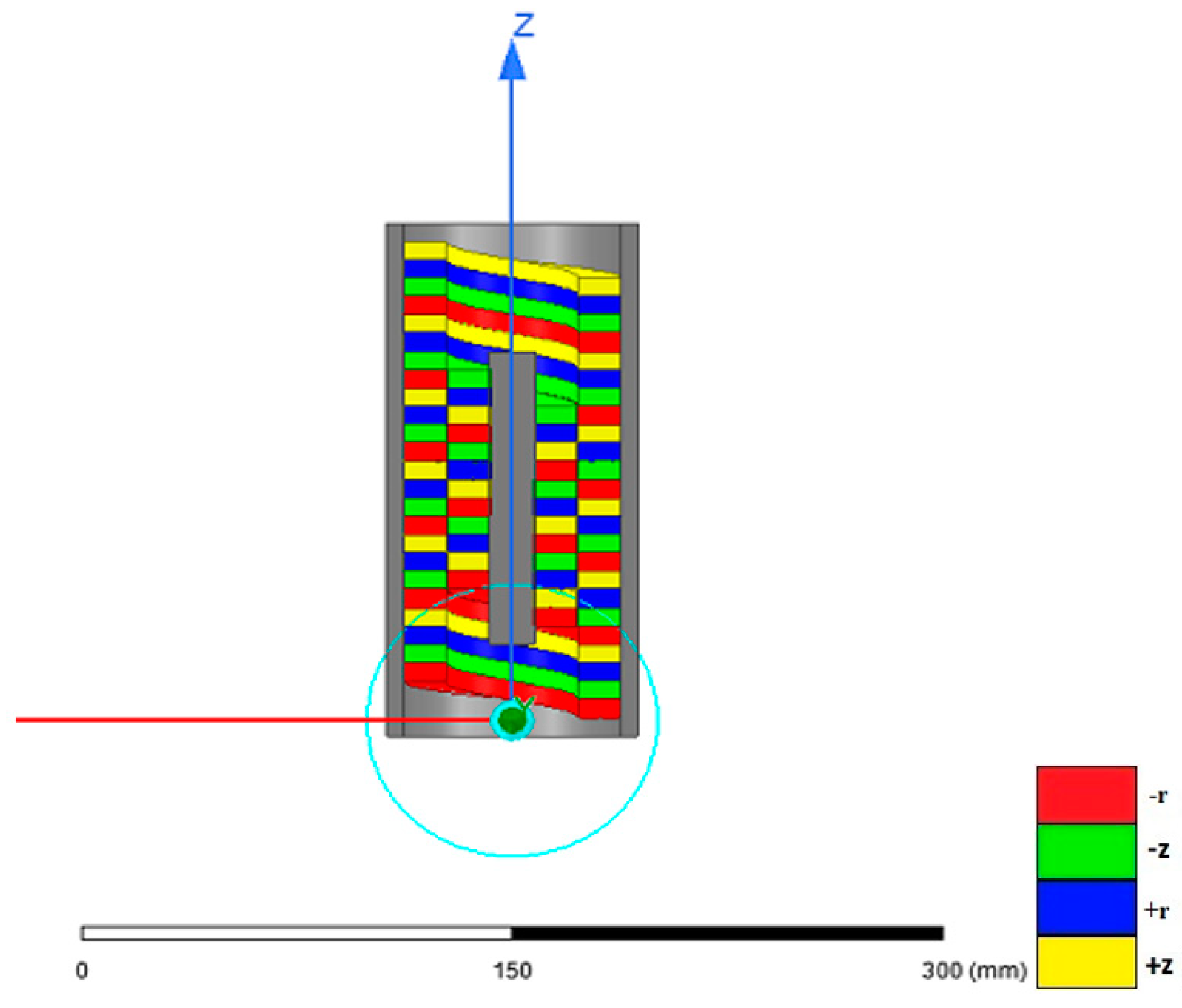
The segmented magnetic arrangement creates a concentrated magnetic flux on the active side of the array while reducing the flux on the passive side [13]. This is possible due to the spatially rotating pattern of the magnetization due to the arrangement of the magnets, thereby rotating the magnetization vector by 90° in the alternate permanent magnet segments, as shown in Figure 2.

Shown in Figure 2 is the configuration that is described in the work below. Both components, the shaft and the ring, have helical permanent magnets in the segmented magnetic arrangement [3,7,10,14,15,23,24]. The red magnet is the radially inward magnetized magnet (−r), green is axially magnetized magnet in the positive direction (+z), the blue magnet is radially outward magnetized magnet (+r), and the yellow magnet is axially magnetized in the negative direction (−z). This sort of arrangement produces the rotating pattern of the magnetization.

2.2. Analytical Modeling

An analytical model of the proposed MLA is developed in this section. The magnetic flux and thrust forces generated during the motion of the shaft through the ring are computed in this model.

2.2.1. Flux Density Model

The magnetic field distribution within the region of the air gap of the MLA will be three-dimensional. With a small air gap, preferably less than the pole pitch which is the length of radially magnetized magnet segment plus the length of the axially magnetized magnet segment, the field distribution can be approximated to be axially symmetric [1,5,17,22].

Based on the magnetic theory, the magnetic field of a permanent magnet is produced by both the regional distributed current as well as the surface distributed current.

From the properties of magnetic field, the region distributed current density is given by

$$\overrightarrow{J_v}=\nabla \times \overrightarrow{M}$$

(2)

and from [17] the surface distributed current density is given by

$$\overrightarrow{J_s}=\left(\overrightarrow{M}-\overrightarrow{M_{air}} \right)\times \overrightarrow{n}$$

(3)

where r is the radial direction and z is the axial direction in Figure 3. Considering the permanent magnet segment as a square of side length l, the angle between the magnetization vector$\overrightarrow{ M}$ and the z direction is α.

Thus, the magnetization vector $\overrightarrow{ M}$ can be expressed as

$$\overrightarrow{ M}=M\mathit{cos}\alpha \overrightarrow{z}+M\mathit{sin}\alpha \overrightarrow{r}$$

(4)

Inside the permanent magnet,

$$\overrightarrow{J_v}=\nabla \times \overrightarrow{M}=0$$

(5)

In the interface between the magnets and the air, the surface distributed current vectors are presented as [17]

$$\begin{gathered} \overrightarrow{J_{s1}}=\overrightarrow{M}\times \left(-\overrightarrow{r}\right)=-M\mathit{cos}\alpha ·\overrightarrow{\mathsf{Ө}} \\ \overrightarrow{J_{s2}}=\overrightarrow{M}\times \left(-\overrightarrow{z}\right)=M\mathit{sin}\alpha ·\overrightarrow{\mathsf{Ө}} \\ \overrightarrow{J_{s3}}=\overrightarrow{M}\times \left(\overrightarrow{r}\right)=M\mathit{cos}\alpha ·\overrightarrow{\mathsf{Ө}} \\ \overrightarrow{J_{s4}}=\overrightarrow{M}\times \left(\overrightarrow{z}\right)=-M\mathit{sin}\alpha ·\overrightarrow{\mathsf{Ө}} \end{gathered}$$

(6)

From [20], for a system with 4-segmented magnets, the magnetization vector is rotated by 90° in different PM segments. Therefore, α takes the values 0°, 90°, 180°, or 270°. Thus, the distributions of magnetization components $M_r$ and $M_z$ can be expressed using a Fourier series representation.

$$\begin{gathered} M_z={\displaystyle \sum }_{k=1,3,5\dots }^{\infty }\frac{4B_r}{{\mu }_{0}k\pi }{A}_{zk}\mathit{sin}\left(\frac{k\pi }{\tau }z\right) \\ {M}_r={\displaystyle \sum }_{k=1,3,5\dots }^{\infty }\frac{4B_r}{{\mu }_{0}k\pi }{A}_{rk}\mathit{cos}\left(\frac{k\pi }{\tau }z\right) \end{gathered}$$

(7)

where, $A_{zk}$ and $A_{rk}$ are given by

$$\begin{gathered} A_{zk}=\mathit{sin}\left(\frac{k\pi }{2}\right)\mathit{sin}\left(\frac{k\pi \left(1-M_R\right)}{2}\right) \\ {A}_{rk}=\mathit{sin}\left(\frac{k\pi }{2}{M}_R\right) \end{gathered}$$

(8)

An analogous structure of the MLA configuration with respect to the shaft and ring is shown in Figure 4 below, where the magnets on ring have surface distributed currents producing the magnetic field. Therefore, the ring is modeled as a slotless stator consisting of rotating rectangular coils with current distribution to form the magnetization of each permanent magnet.

The following assumptions are considered for the derivation of the analytical solution of magnetic field distribution in the MLA.

• Magnetic field distributions are calculated from the product of magnetic field intensity produced by the magnetic segments and the relative permeance at any position;
• The permeability of the back irons of the ring and shaft is infinite;
• Air gap length is small, so that the magnetic field distribution can be approximated as axially symmetric;
• The back-iron is not saturated and the eddy current and the hysteresis losses in the back irons in the system are neglected;
• Magnet thickness is the same for the ring and shaft magnets;
• The magnetic field distribution calculations and the thrust force calculations are two dimensional (2D). The 2D results are same for 3D, which is validated using FEA.

The magnet segments on the ring are considered to be rectangular, current-carrying coils with surface current density. The model includes three regions, in particular (I) air gap; (II) permanent magnets; (III) back iron.

From [20], the flux density $\overrightarrow{B}$ in tesla and the flux intensity, $\overrightarrow{H}$ in ampere per meter in the regions I, II and III are:

$$\overrightarrow{B_I}={\mu }_0\overrightarrow{H_I}$$

(9)

$$\overrightarrow{B_{II}}={\mu }_r{\mu }_0\overrightarrow{H_{II}}+{\mu }_0\overrightarrow{M}$$

(10)

$$\overrightarrow{B_{III}}={\mu }_0{\mu }_{iron}\overrightarrow{H_{III}}$$

(11)

where, ${\mu }_r$ and ${\mu }_{iron}$ are relative permeabilities.

The magnetic field intensity vectors relative to z and r directions, given by $H_z$ and $H_r$, are derived from the magnetic scalar potential ($\phi$)

$$H_z=-\frac{\partial \phi }{\partial z} \mathrm{and} H_r=-\frac{\partial \phi }{\partial r}$$

(12)

The distribution in regions I, II and III are all governed by the Laplace equation in two-dimension as

$$\frac{{\partial }^2\phi }{\partial z^2}+\frac{{\partial }^2\phi }{\partial r^2}=0$$

(13)

The distribution of the magnetization components $M_r$ and $M_z$ is homogeneous harmonic distribution. From [20], the solution for magnetic scalar potential in the different regions are given as

$${\phi }_n\left(r,z\right)={\displaystyle \sum }_{k=1,3,5\dots }^{\infty }\left(A_{nk}{e}^{k\frac{\pi }{\tau }r}+B_{nk}{e}^{-k\frac{\pi }{\tau }r}\right)\mathit{cos}\left(k\frac{\pi }{\tau }z\right)$$

(14)

where, n = 1, 2 or 3, referring to the three regions, and the parameters $A_{nk}$ and $B_{nk}$ are the constants in those regions to be calculated using the boundary conditions. The back-iron is ignored in the model assuming infinite permeability. Therefore, the synthetic boundary condition on the surface (r = R_s) is the Neumann boundary condition, where the permeability of iron is greater than that of air. Additionally, the Dirichlet boundary condition is adopted in the region r = R₀.

Therefore

$$\begin{gathered} B_{zI}\left(r,z\right){|}_{r=R_s}=0 \\ {B}_{rIII}\left(r,z\right){|}_{r=R_o}=0 \end{gathered}$$

(15)

where, $B_r$ and $B_z$ are respectively the r and z direction components of $\overrightarrow{B}$.

From [20], because $B_{zII}\left(r,z\right)$ and $B_{rII}\left(r,z\right)$ are both governed by (10), the boundary conditions between R_r and R_m2 shall be complicated and therefore, the expressions for the magnetic field distributions will be difficult to solve. Hence, adopting the synthetic boundary conditions at r = R_r and r = R_m2 results in a simpler model. $M_r$ is governed by (7) and $M_z$ is replaced by a virtual equivalent surface current $J_s$ which is given by:

$$J_s=\frac{M_z}{{\mu }_r}$$

(16)

Then, the synthetic boundary conditions at r = R_r and r = R_m2 are as follows:

$$H_{zI}\left(r,z\right){|}_{r=R_{m2}}=H_{zII}\left(r,z\right){|}_{r=R_{m2}}+\frac{M_z}{{\mu }_r}$$

(17a)

$$B_{rI}\left(r,z\right){|}_{r=R_{m2}}=B_{rII}\left(r,z\right){|}_{r=R_{m2}}$$

(17b)

$$H_{zIII}\left(r,z\right){|}_{r=R_r}=H_{zII}\left(r,z\right){|}_{r=R_r}+\frac{M_z}{{\mu }_r}$$

(17c)

$$B_{rIII}\left(r,z\right){|}_{r=R_r}=B_{rII}\left(r,z\right){|}_{r=R_r}$$

(17d)

Solving (13), the general solutions in the three regions and on the surface of the stator core, subjected to the distributions of the magnetization components in (7) and the boundary conditions (15) and (17a,b,c,d), are provided below.

Flux density in airgap and synthetic ring coils Region I -

$$B_{zI}\left(r,z\right)={{\displaystyle \sum }}_{k=1,3,5}^{\infty }\frac{4B_r}{k\pi }\left(A_{rk}-\frac{E_b{E}_d-e^{-k\frac{\pi }{\tau }{h}_m}{E}_e{E}_a+e^{-k\frac{\pi }{\tau }{h}_m}{E}_e{E}_c-e^{-2k\frac{\pi }{\tau }{h}_m}{E}_b{E}_f}{E_d{E}_c-e^{-2k\frac{\pi }{\tau }{h}_m}{E}_a{E}_f}\right)\left(\frac{e^{2k\frac{\pi }{\tau }\left(r-R_s\right)}-1}{e^{-2k\frac{\pi }{\tau }{h}_g}+1}\right)e^{k\frac{\pi }{\tau }\left(R_{m2}-r\right)}\mathit{sin}\left(k\frac{\pi }{\tau }z\right)$$

(18a)

$$B_{rI}\left(r,z\right)={{\displaystyle \sum }}_{k=1,3,5}^{\infty }\frac{4B_r}{k\pi }\left(A_{rk}-\frac{E_b{E}_d-e^{-k\frac{\pi }{\tau }{h}_m}{E}_e{E}_a+e^{-k\frac{\pi }{\tau }{h}_m}{E}_e{E}_c-e^{-2k\frac{\pi }{\tau }{h}_m}{E}_b{E}_f}{E_d{E}_c-e^{-2k\frac{\pi }{\tau }{h}_m}{E}_a{E}_f}\right)\left(\frac{e^{2k\frac{\pi }{\tau }\left(r-R_s\right)}+1}{e^{-2k\frac{\pi }{\tau }{h}_g}+1}\right)e^{k\frac{\pi }{\tau }\left(R_{m2}-r\right)}\mathit{cos}\left(k\frac{\pi }{\tau }z\right)$$

(18b)

Flux density in Permanent magnet Region II -

$$B_{zII}\left(r,z\right)={{\displaystyle \sum }}_{k=1,3,5}^{\infty }\frac{4B_r}{k\pi }\left(A_{rk}-\frac{e^{k\frac{\pi }{\tau }\left(r-R_{m2}\right)}{E}_b{E}_d-e^{k\frac{\pi }{\tau }\left(r-R_{m2}-h_m\right)}{E}_e{E}_a-e^{k\frac{\pi }{\tau }\left(R_r-r\right)}{E}_e{E}_c+e^{k\frac{\pi }{\tau }\left(R_r-r-h_m\right)}{E}_b{E}_f}{E_d{E}_c-e^{-2k\frac{\pi }{\tau }{h}_m}{E}_d{E}_f}\right)\mathit{sin}\left(k\frac{\pi }{\tau }z\right)$$

(19a)

$$B_{rII}\left(r,z\right)={{\displaystyle \sum }}_{k=1,3,5}^{\infty }\frac{4B_r}{k\pi }\left(A_{rk}-\frac{e^{k\frac{\pi }{\tau }\left(r-R_{m2}\right)}{E}_b{E}_d-e^{k\frac{\pi }{\tau }\left(r-R_{m2}-h_m\right)}{E}_e{E}_a+e^{k\frac{\pi }{\tau }\left(R_r-r\right)}{E}_e{E}_c-e^{k\frac{\pi }{\tau }\left(R_r-r-h_m\right)}{E}_b{E}_f}{E_d{E}_c-e^{-2k\frac{\pi }{\tau }{h}_m}{E}_d{E}_f}\right)\mathit{cos}\left(k\frac{\pi }{\tau }z\right)$$

(19b)

Flux density in back iron Region III -

$$B_{zIII}\left(r,z\right)={{\displaystyle \sum }}_{k=1,3,5}^{\infty }\frac{4B_r}{k\pi }\left(A_{rk}-\frac{e^{-2k\frac{\pi }{\tau }{h}_m}{E}_e{E}_a-e^{-k\frac{\pi }{\tau }{h}_m}{E}_b{E}_d-E_e{E}_c+e^{-k\frac{\pi }{\tau }{h}_m}{E}_b{E}_f}{e^{-2k\frac{\pi }{\tau }{h}_m}{E}_a{E}_f-E_d{E}_c}\right)\left(\frac{e^{-2k\frac{\pi }{\tau }\left(r-R_0\right)}+1}{e^{-2k\frac{\pi }{\tau }{h}_g}-1}\right)e^{-k\frac{\pi }{\tau }\left(R_r-r\right)}\mathit{sin}\left(k\frac{\pi }{\tau }z\right)$$

(20a)

$$B_{rIII}\left(r,z\right)={{\displaystyle \sum }}_{k=1,3,5}^{\infty }\frac{4B_r}{k\pi }\left(A_{rk}-\frac{e^{-2k\frac{\pi }{\tau }{h}_m}{E}_e{E}_a-e^{-k\frac{\pi }{\tau }{h}_m}{E}_b{E}_d-E_e{E}_c+e^{-k\frac{\pi }{\tau }{h}_m}{E}_b{E}_f}{e^{-2k\frac{\pi }{\tau }{h}_m}{E}_a{E}_f-E_d{E}_c}\right)\left(\frac{e^{-2k\frac{\pi }{\tau }\left(r-R_0\right)}-1}{e^{-2k\frac{\pi }{\tau }{h}_g}-1}\right)e^{-k\frac{\pi }{\tau }\left(R_r-r\right)}\mathit{cos}\left(k\frac{\pi }{\tau }z\right)$$

(20b)

where

$$E_a=\left(e^{-2k\frac{\pi }{\tau }{h}_g}-1\right)+\frac{1}{{\mu }_r}\left(e^{-2k\frac{\pi }{\tau }{h}_g}+1\right)$$

(21a)

$$E_b=A_{zk}\frac{1}{{\mu }_r}\left(e^{-2k\frac{\pi }{\tau }{h}_g}+1\right)+A_{rk}\left(e^{-2k\frac{\pi }{\tau }{h}_g}-1\right)$$

(21b)

$$E_c=\left(e^{-2k\frac{\pi }{\tau }{h}_g}-1\right)-\frac{1}{{\mu }_r}\left(e^{-2k\frac{\pi }{\tau }{h}_g}+1\right)$$

(21c)

$$E_d=\left(e^{-2k\frac{\pi }{\tau }{h}_b}+1\right)+\frac{{\mu }_{iron}}{{\mu }_r}\left(1-e^{-2k\frac{\pi }{\tau }{h}_b}\right)$$

(21d)

$$E_e=A_{zk}\frac{{\mu }_{iron}}{{\mu }_r}\left(e^{-2k\frac{\pi }{\tau }{h}_b}+1\right)+A_{rk}\left(e^{-2k\frac{\pi }{\tau }{h}_b}+1\right)$$

(21e)

$$E_f=\left(e^{-2k\frac{\pi }{\tau }{h}_b}+1\right)-\frac{{\mu }_{iron}}{{\mu }_r}\left(1-e^{-2k\frac{\pi }{\tau }{h}_b}\right)$$

(21f)

In the above equations, the thickness of the air gap is given by h_g = R_m1 − R_m2, the thickness of the magnetic section is h_m = R_m2 − R_r, and the thickness of the back iron is h_b = R_r − R₀.

2.2.2. Thrust Force Calculations

Based on the work in [3] for an MLA system, with the flux density model developed in this work, the thrust force can now be computed. The magnets on the outer rotor ring can be represented by current carrying coils distributed on both sides of the magnets. The equivalent current density, J_c is given as [7,10]

$$J_c=\frac{B_r}{{\mu }_0{\mu }_r}$$

(22)

where, B_r is the remanence (T), ${\mu }_0$ is the permeability in vacuum (H/m) and ${\mu }_r$ is the relative permeability (non-dimensional).

From [10,17], the thrust force $F$, acting on the ring as a result of interaction of the magnetic field on shaft and the equivalent current on ring, is given by:

$$F=\oint \left(J_c\times B\right)dS$$

where, $S$ is the surface area of the current sheet.

Thus, referring to [10,17], the thrust force to be calculated, acting on the pole of the ring due to the interaction of the magnetic field produced and the equivalent current model on the shaft is given as

$$F_{pole}=\oint \left(J_{ci}\times B\right)dS$$

(23)

where, i= 1, 2, 3, 4 indicate the surfaces, $S_1$, $S_2$, $S_3$ and $S_4$ as shown in Figure 5.

Therefore, the total thrust force acting on one pole of the ring is given by

$$F_{pole}=F_1+F_2+F_3+F_4=\oint \left(J_{c1}\times B\right)dS+\oint \left(J_{c2}\times B\right)dS+\oint \left(J_{c3}·B\right)dS+\oint \left(J_{c4}·B\right)dS$$

(24)

where, $S$ is the surface area of the current sheet for sides 1,2,3 and 4, indicated as $S_1$, $S_2$, $S_3$ and $S_4$.

From (6)

$$\begin{gathered} \overrightarrow{J_{c1}}=\overrightarrow{J_{c3}}=\frac{B_r}{{\mu }_0{\mu }_r}·\overrightarrow{\mathsf{Ө}} \\ \overrightarrow{J_{c2}}=\overrightarrow{J_{c4}}=-\frac{B_r}{{\mu }_0{\mu }_r}·\overrightarrow{\mathsf{Ө}} \end{gathered}$$

(25)

To proceed to the total force calculation, consider: (1) the force acting on the radially oriented magnets ($F_1+F_2$), and (2) the force acting on the axial-oriented magnets of the segmented magnetic array pole ($F_3+F_4$).

Therefore, from [7,10], and from (18b) and (23)

$$F_1+F_2={\displaystyle \sum }_{k=1,3,5}^{\infty }4\pi J_c{I}_{rkI}\mathit{sin}\left(\frac{k\pi }{\tau }\frac{{\tau }_r}{2}\right)\mathit{cos}\left(\frac{k\pi }{\tau }{z}_d\right)$$

(26)

where, $z_d$ is the axial displacement of the radial-oriented magnetic segment on the ring with respect to the radial-oriented magnetic segment on the shaft, and ${\tau }_r$ is the axial length of the radial magnet segment.

The variable $I_{rkI}$ is the main component variable of the force equation acting on radial-oriented magnets, given by

$$I_{rkI}=\left(i_1+i_2\right)i_{rk}$$

(27)

where, $i_{rk}$ is the common component variable of the force equation acting on radial-oriented magnets and axial-oriented magnets, given by

$$i_{rk}=\frac{4B_r}{k\pi }\left(A_{rk}-\frac{E_b{E}_d-e^{-k\frac{\pi }{\tau }{h}_m}{E}_e{E}_a+e^{-k\frac{\pi }{\tau }{h}_m}{E}_e{E}_c-e^{-2k\frac{\pi }{\tau }{h}_m}{E}_b{E}_f}{E_d{E}_c-e^{-2k\frac{\pi }{\tau }{h}_m}{E}_a{E}_f}\right)\left(\frac{1}{e^{-2k\frac{\pi }{\tau }{h}_g}+1}\right)$$

(28)

$$i_1=\left(\frac{\tau }{k\pi }\right)\left(R_s{e}^{k\frac{\pi }{\tau }\left(R_{m2}-R_s\right)}-R_{m1}{e}^{k\frac{\pi }{\tau }\left(R_{m2}+R_{m1}-2R_s\right)}\right)-{\left(\frac{\tau }{k\pi }\right)}^2\left(e^{k\frac{\pi }{\tau }\left(R_{m2}-R_s\right)}-e^{k\frac{\pi }{\tau }\left(R_{m2}+R_{m1}-2R_s\right)}\right)$$

(29)

$$i_2=\left(\frac{\tau }{k\pi }\right)\left(R_{m1}{e}^{k\frac{\pi }{\tau }\left(R_{m2}-R_{m1}\right)}-R_s{e}^{k\frac{\pi }{\tau }\left(R_{m2}-R_s\right)}\right)-{\left(\frac{\tau }{k\pi }\right)}^2\left(e^{k\frac{\pi }{\tau }\left(R_{m2}-R_s\right)}-e^{k\frac{\pi }{\tau }\left(R_{m2}-R_{m1}\right)}\right)$$

(30)

where $i_1$ and $i_2$ are sub-component variables in the force calculations.

Also, from (18a) and (23)

$$F_3+F_4={\displaystyle \sum }_{k=1,3,5}^{\infty }4\pi J_c{I}_{rkII}\mathit{sin}\left(\frac{k\pi }{\tau }\left(\frac{\tau -{\tau }_r}{2}\right)\right)\mathit{sin}\left(\frac{k\pi }{\tau }\left(z_d-\frac{\tau }{2}\right)\right)$$

(31)

where $I_{rkII}$ is main-component variable of force acting on axial-oriented magnets, given by

$$I_{rkII}=\left(i_1-i_2\right)i_{rk}$$

(32)

Thus, (24) can be re-written as

$$\begin{gathered} F_{pole}=\left[{\displaystyle \sum }_{k=1,3,5}^{\infty }4\pi J_c{I}_{rkI}\mathit{sin}\left(\frac{k\pi }{\tau }\frac{{\tau }_r}{2}\right)\mathit{cos}\left(\frac{k\pi }{\tau }{z}_d\right)\right] \\ +\left[{\displaystyle \sum }_{k=1,3,5}^{\infty }4\pi J_c{I}_{rkII}\mathit{sin}\left(\frac{k\pi }{\tau }\left(\frac{\tau -{\tau }_r}{2}\right)\right)\mathit{sin}\left(\frac{k\pi }{\tau }\left(z_d-\frac{\tau }{2}\right)\right)\right] \end{gathered}$$

(33)

where $F_{pole}$ is the force for a single pole in an infinite long array without any edge effect losses or interaction losses, which are the ideal conditions. The peak magnetic flux magnitude is associated with a single pole or a few poles, in a multi-pole system, and the thrust force due to that peak magnetic performance of a single or a few individual poles can be calculated using (33). However, in a multi-pole system, equation (33) cannot be simply multiplied by the number of active poles to calculate the magnetic thrust force of the entire MLA system, due to the existence of magnetic flux losses, explained in further sections.

3. Pole Corrections Calculations

After analytically calculating the thrust force experienced by one pole of the ring in an infinite long array without any losses, to calculate the total thrust force experienced by the ring, the force on one pole is multiplied by the number of poles as seen in previous works [3,7]. This is the methodology used in previous works with the conventional magnetic arrangement, as the error would be negligible for an MLA with a large number of poles and small embodiments of the ring and shaft framework [3,7].

However, upon further investigation on various ring-shaft systems of varying dimensions, it was found that not all of the active poles contribute to the thrust force calculations equally. Thus, simply multiplying with the number of active poles could potentially over-estimate the thrust force of the system because the poles on both ends of the ring and shaft system were not contributing to the flux field as were the poles in the middle.

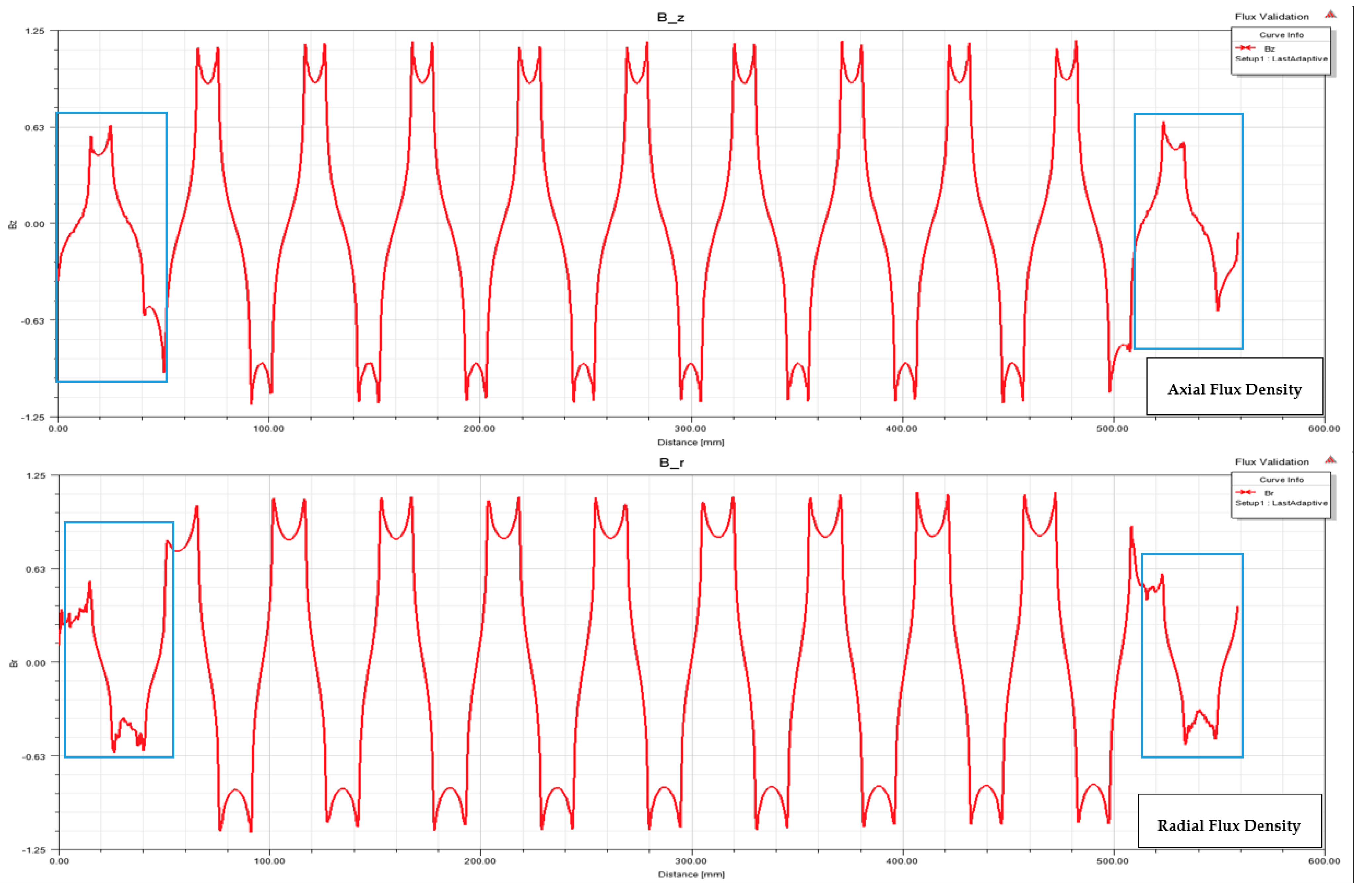
A multi-pole MLA with segmented magnetic arrangement in vacuum illustrates the flux density plots in Figure 6 for one shaft. The axial flux density and the radial flux density plots indicate that the poles at the edges contribute lower resultant flux than the poles at the center of the ring-shaft system. This is due to the magnetic flux losses at the ends where for the segmented magnetic field lines; there is no further magnetization field to connect to and, thus, in a way it mitigates gradually. For these edge conditions and observed interaction conditions, an analysis was conducted to quantify the losses under different conditions, such as positioning, dimensional variations, changing the air gap, and increase of the number of active poles.

The same conditions are seen when the model is tested with different sizes for ring and shaft, with segmented magnet array, and with different number of active leads. For a longer actuator with a higher number of leads, the edge losses may extend to other poles that are farther away from the edges, towards the center of the embodiment. In some cases, significant losses in magnetic flux appeared in more than three poles away from the edges, compared to the flux of the poles at the center. Since the shaft in this study has fewer magnet leads compared to the ring, the edge conditions present themselves on the edges of the extreme ends of magnetic arrangement on the shaft. If the ring has fewer number of magnetic leads than the shaft, then the ring will present these edge conditions instead, as the fewer magnetic leads on the ring interact with only a few numbers of magnetic leads on the shaft.

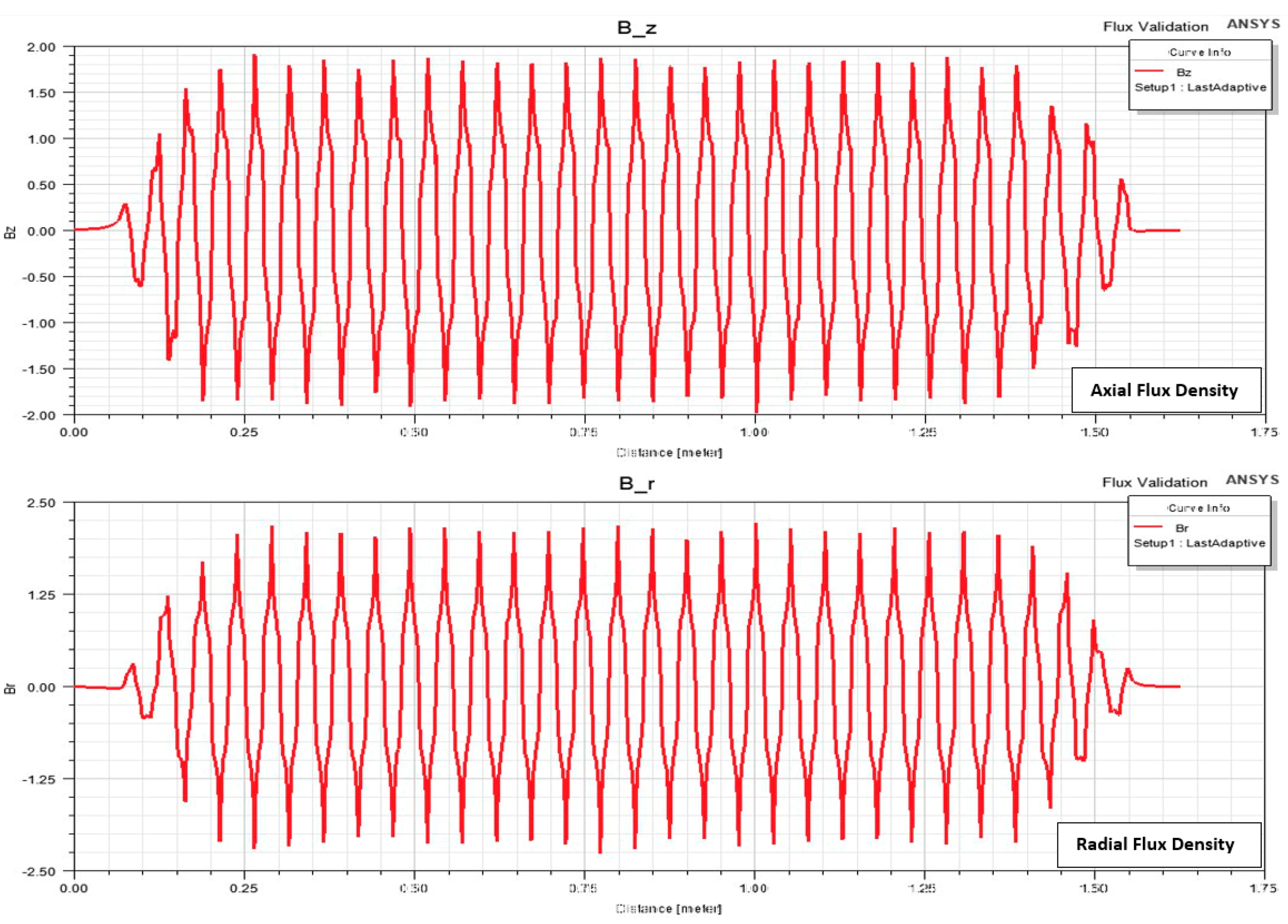
In a multi-pole magnetic flux plot for the interacting ring and shaft arrangement, it can be observed that the peaks of the resultant magnetic fields of the arrangement, for each individual pole, do not remain consistent with the maximum flux peak obtained during the interaction, as calculated by the single pole calculations from the subdomain model under ideal conditions. This constitutes the observed magnetic interaction effect, presented in Figure 7.

It should be noted that these observed interaction effects, together with the edge conditions, are collectively called the magnetic Flux Effects, which can only be modeled via FEA.

A visual representation of the observed interaction condition is presented in Figure 7. The observed interaction condition remains the same whether if the ring or the shaft have higher relative number of leads with respect to each other and increases with increase in number of poles directly.

To account for these magnetic Flux Effects, or losses, the Pole Correction Factor ($P_C$) is introduced and subtracted from the total number of poles $\left(p\right)$ engaged between the ring and the shaft, and the following expression is employed

$$\left(p-P_C\right)·F_{Pole}=F_{FEA}$$

(34)

Equation (34) can be written as

$$P_C=p-\frac{F_{FEA}}{F_{Pole}}$$

(35)

where, $F_{FEA}$ is the result from the FEA modeling for a system with $p$ number of poles and $F_{Pole}$ is calculated analytically for one pole as explained in (33). The pole correction factor P_c accounts for the correction of poles required to predict the accurate result.

To account for these losses in the flux density and to formulate a robust mathematical model, systematic analysis of the data was conducted to reproduce the actual edge conditions and interaction conditions analytically.

For this analysis, varying dimensions, such as different air gaps, segmented magnet lead lengths and thicknesses of the magnet and the back-iron, were considered and analyzed via the Finite element analysis. The FEA modeling was conducted in Ansys electronics desktop 2020R2, where the ring and shaft embodiments were simulated to produce the results for the net thrust force exerted by the ring on the shaft. The solution convergence is determined at less than 1% energy error in Ansys Maxwell. The results were compared with the resultant thrust force, calculated analytically per pole, using the model presented above. The variations noted, with different physical aspects in view, and the geometric ratios were considered. Using the Buckingham π theorem, all sets of possible non-dimensional geometric ratios, or π groups, were studied for parametric model identification of these losses in the system.

Using the π groups to analyze the variations in the analytical result and the FEA result, with respect to the variations in these π groups, a linear regression model was calculated iteratively for calculation of the losses using a combinatorial iterations methodology, assessing different combinations of the non-dimensional π groups produced earlier. The number of dimensional parameters needed to fulfill this analysis were iteratively selected, and each of these non-dimensional π groups represent ratios of dimensional parameters from the gathered data. The developed formulation accounts for the losses that were prevalent in all the three-dimensional embodiments assessed in this study. Using $P_C$, which accounts for the correction of poles required to predict the accurate result and therefore, is a parameter for losses correction; a normalized correction factor was developed and assessed iteratively with the π groups discovered before.

The formula that was generated that included the non-linear relationship of the Actual Pole Correction Normalized factor, called $P_C{N}_{Actual}$.

Equation (34) can be re-written as

$$\left(1-\frac{P_C}{p}\right)=\frac{F_{FEA}}{p·F_{Pole}}=P_C{N}_{Actual}$$

(36)

For $m$ number of leads, the number of poles, $p$, is equal to twice the number of leads, i.e., $p=2·m$.

The variation in the losses with the varying π groups is narrowed down iteratively to the π groups having the most influence on this estimation, presented in

Table 1. π groups having most influence on edge conditions and interaction conditions (Dimensionless).

π Groups	Dimensionless Value
π1	($\lambda$ /Rm1)
π2	(hg/$\lambda$)
π3	(MR—0.5)

. This was accomplished by minimizing the percent error between the actual value (FEA) and the estimate, iteratively via parametric model regression of the Estimated Pole Correction Normalized factor, $P_C{N}_{Estimated}$, with respect to the different π groups. An error histogram is presented in Figure 8.

The value for $P_C{N}_{Estimated}$ was calculated as:

$$P_C{N}_{Estimated}=1.0108-0.2183·{\pi }_1+\left(0.045367·{\pi }_1{}^2\right)-{\pi }_3·M_{MR}$$

(37)

where $M_{MR}$ is the residual model for varying magnet ratios from greater than 0.5 to a magnet ratio of 0.8 and is given as:

$$M_{MR}=0.51259+0.15048·{\pi }_1-\left(0.35488·{\pi }_1{}^2+3.2253\right)·{\pi }_2$$

(38)

Therefore, the thrust force for $p$ number of poles system in Table 1, given below, is analytically calculated as:

$$F_{Thrust}=p·P_C{N}_{\mathit{Estimated}}·F_{pole}$$

(39)

where $F_{pole}$ is the single pole thrust force given by (33).

This model was used to calculate the value of thrust force exerted by the shaft onto the ring, accounting for the edge conditions and the interaction conditions, and was validated for different embodiments with different dimensions and magnet grades via Finite Element Analysis. Out of the 650+ FEA studies conducted for this study, 368 cases were used for validation of the model concerning manufacturable embodiments of the MLA. Prediction accuracy will tend to be an overfit if more cases are used for calibration than used in the study. In the presented investigation, the range was set for the modeling parameters to prevent any non-practical geometry dimensions of the MLA system. This model is calibrated for the range presented in

Table 2. Model Calibration Ranges.

Parameters	Variable Descriptions	Variable Range
π1	($\lambda$/Rm1)	($\lambda$/Rm1) ∈ (0.14,3)
π2	(hg/$\lambda$)	(hg/$\lambda$) ∈ (0.01,0.125)
π3	(MR—0.5)	MR ∈ [0.5,0.8]
π4	(λ/hm)	(λ/hm) ∈ (0.4,10)
Airgap	hg	hg ≤ 2 mm

.

The limits for π₁ and π₄ ensure that the three-dimensional embodiment is not a superficial design where the shaft is too thick or too thin relative to the magnet thickness. The limits of π₂ ensures that the airgap is not too large relative to the lead of the magnetic arrangement. The model has been calibrated to a maximum value of 2 mm for airgaps; anything more shall only deteriorate the efficiency of the MLA system and is not a good practice. Among the validation dataset, the maximum error between $P_C{N}_{Actual}$ from (36) and the obtained $P_C{N}_{Estimated}$ from (37), was observed to be 5.6%, as shown in Figure 9. The 5.6% error for a case with 2mm airgap and a 5.1% error for a case with 0.8 magnet ratio—two scenarios at the boundaries of the ranges presented in Table 2.

The derived model has been validated for different Neodymium Iron Boron magnet grades [25].

The properties of different magnet grades are presented in Figure 10. Magnets with various grades as listed have been employed in the MLA system force modeling, which have been validated by FEA simulations. The percent errors of the model estimate compared to the actual force results (via FEA) were all under 5%.

Another term from the $P_{C}N$ calculations that can be obtained is the utilized magnet efficiency, or the magnet volume efficiency in the MLA system, corresponding to the utilization and performance of the system with respect to the magnetic material volume present. From (36):

$$\left(1-\frac{P_C}{p}\right)=\frac{F_{FEA}}{p·F_{Pole}}=P_C{N}_{Actual}$$

where, $\frac{P_C}{p}$ is the ratio of the pole correction required over the total number of poles in the system. In MLA scenarios with lower $P_C$, the edge loss of the magnetic flux would be less significant, and therefore, the loss of the thrust force is less compared to the cases when $P_C$ is high. In such case, the utilization of magnets in the MLA system becomes more efficient to generate the thrust force, which causes a high magnetic utilized efficiency. In this study, (37) presents the estimation of $P_C{N}_{\mathit{Actual}}$, based on the beforementioned π groups, as $P_C{N}_{\mathit{Estimated}}$. Therefore, this magnet volume efficiency of the system depends directly upon $P_C{N}_{\mathit{Estimated}}$ and is given by:

$$\mathsf{ɳ}=\left(P_C{N}_{Estimated}·100\right)\%$$

(40)

4. Results and Validation

Following the formulation of the analytical expression for the magnetic flux, the thrust force calculations and the identification of edge conditions, and the interaction conditions based on the ratios π₁ (λ /Rm₁) and π₃ (λ /t), the validation of the entire computed model was conducted by finite element analysis in Ansys electronics desktop 2020R2, restrained to solution convergence at less than 1% energy error. An MLA system example is analyzed here, calculating the maximum magnetic thrust force, with analytical calculation (no flux loss), the present model (with flux loss), and FEA simulation, respectively.

Consider the MLA dimensions and parameters in

Table 3. Input Design Parameters (sample).

Description	Units	Value
Number of Leads on Ring	N/A	6
Number of Leads on Shaft	N/A	3
MLA Outer Diameter	mm	89.5
Shaft Back Iron Thickness, hb	mm	8
Ring Back Iron Thickness	mm	6
Magnet Thickness, hm	mm	15
Air-Gap Length, hg	mm	0.75
Lead, λ	mm	28
Pole Length, τ	mm	14
Magnet Grade	N/A	N48H
Remanence, Br	T	1.39
Rel. Permeability, μr	N/A	1.06
Magnet Ratio, MR	N/A	0.5
Length of the Ring	mm	196
Length of the Shaft	mm	112

, for which the results from the analytical model and the FEA are presented and compared below.

From Figure 11, there are three leads or six poles that are active at a time and are responsible for exerting force. The poles at the edges are the lesser contributing participants in the equivalent current-carrying coil system. The poles other than at the edges have inconsistent interaction losses, which are not visible in the equivalent current-carrying coil system but can be visually seen in the magnet-to-magnet flux interaction plot in Figure 7.

Figure 12 presents the individual magnetic arrangements on both the shaft and the ring, which are helically mounted on the outer surface of the shaft and the inner surface of the ring, respectively.

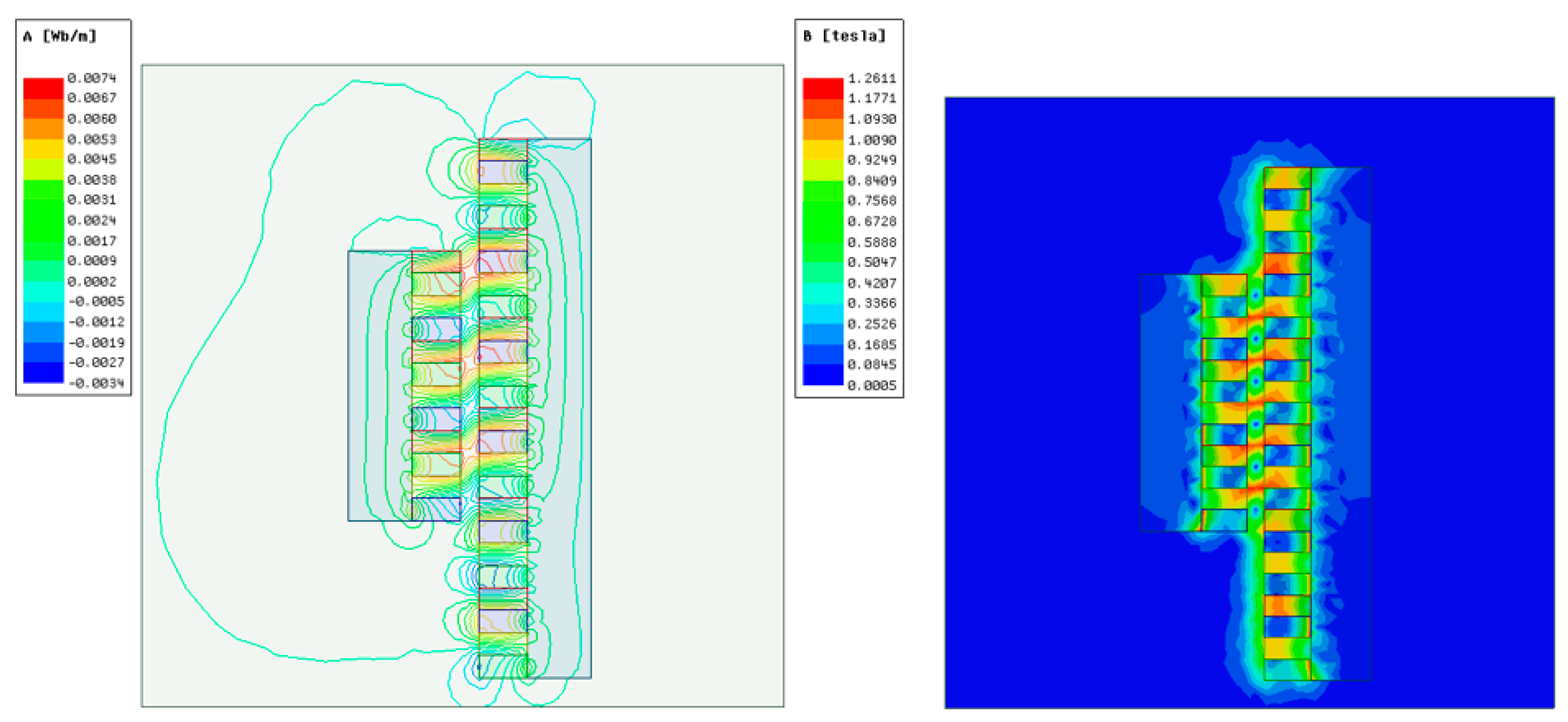
From the FEA, the 2D magnetic field distribution is shown in Figure 13 which includes both the ring and the shaft. This magnetic flux representation is in 2D because the 3D representation will be chaotic to visualize.

The figures below show the flux density calculations for the shaft from the analytical model, (18a) and (18b), as function of the axial displacement.

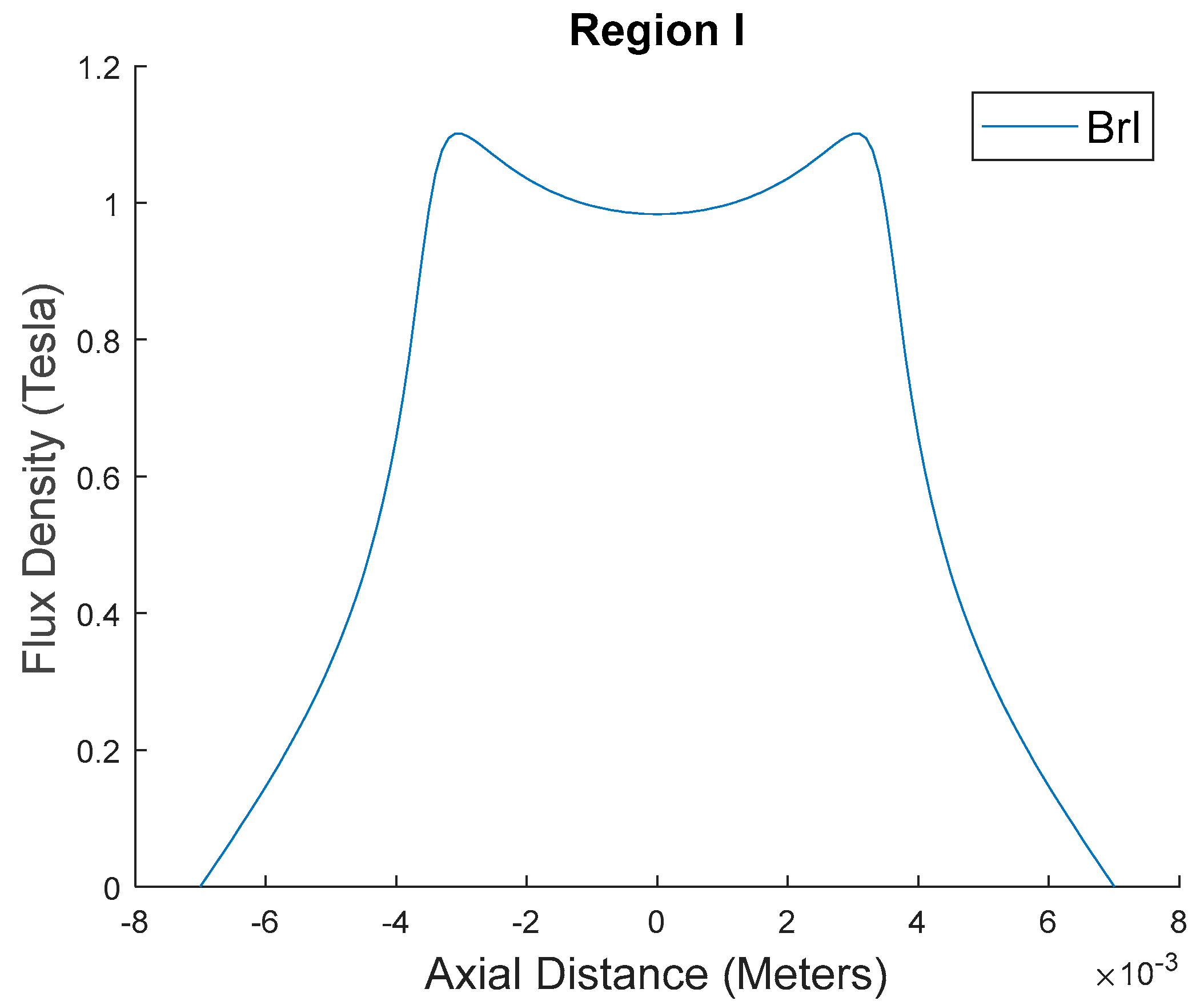
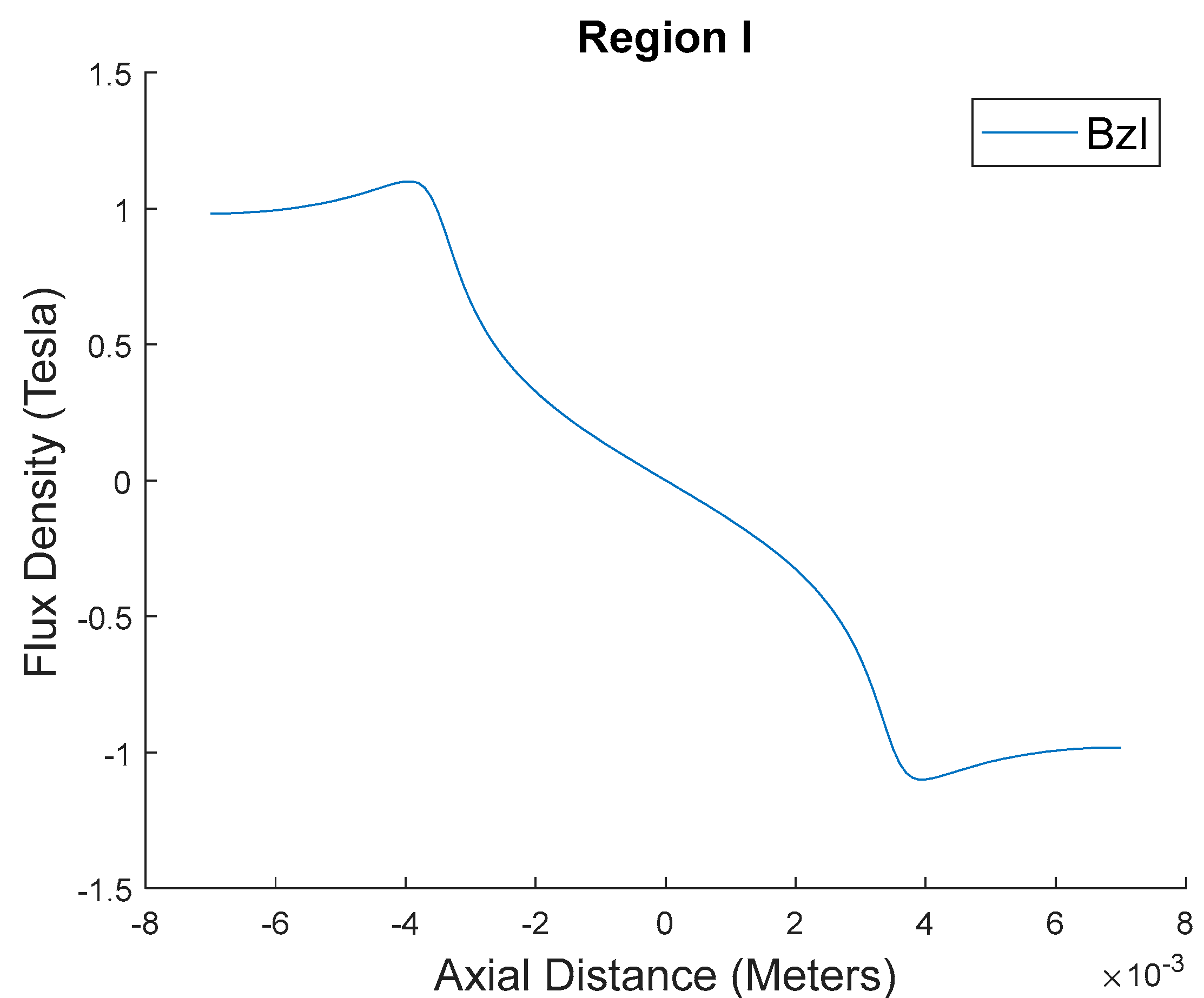
The wave forms for the magnetic flux density in the region of the air gap are presented above in Figure 14 and Figure 15 for the radial flux density and the axial flux density, respectively.

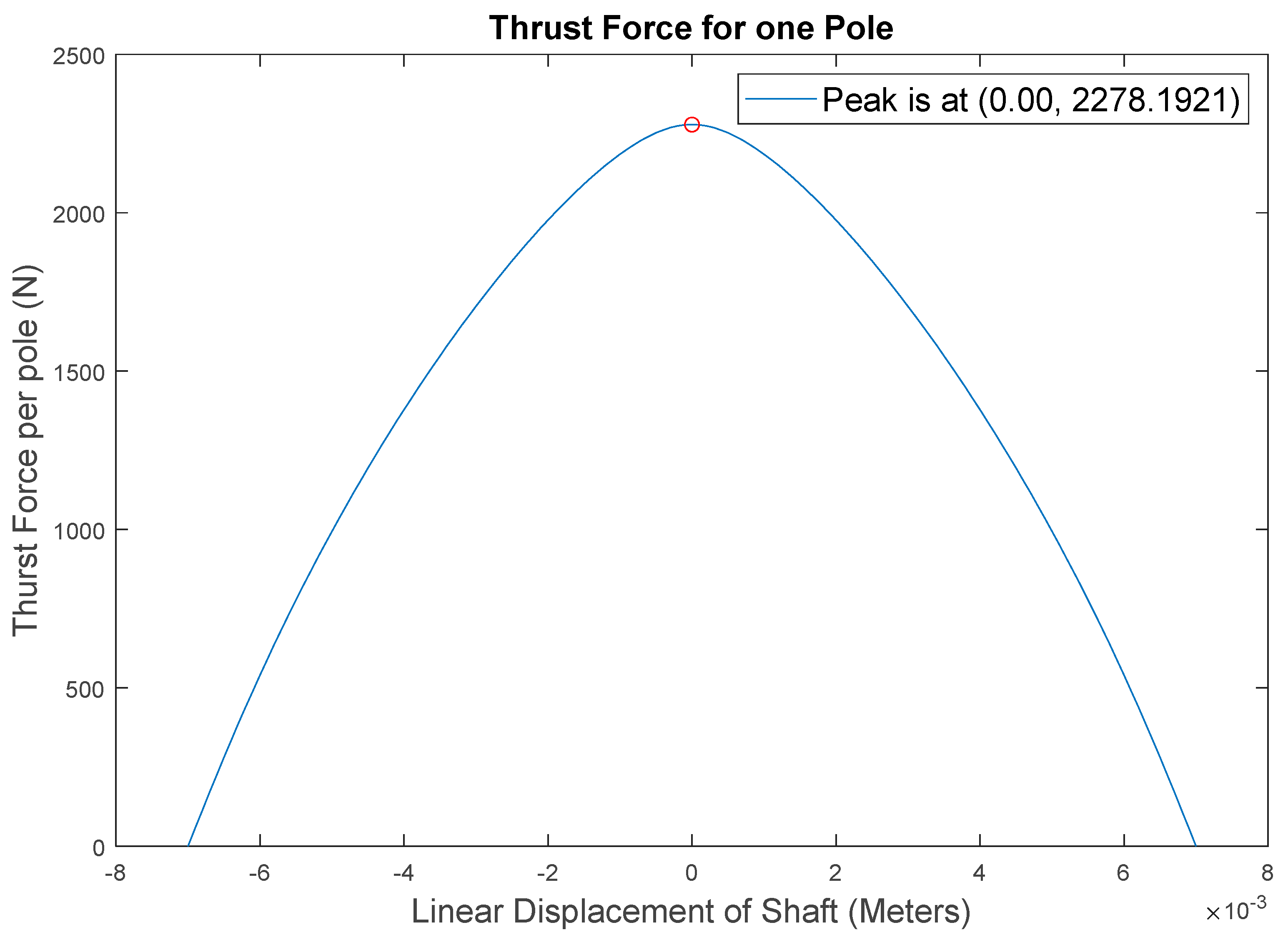
When the pole displacement is zero, or half the lead, the resultant thrust force is nearly zero. It is only when the pole displacement starts to rise from zero that the system experiences force due to the magnetic flux interactions among the various segmented array magnetic poles. The thrust force peak shown for one pole in Figure 16 is achieved when the relative displacement of the ring with respect to the shaft, or vice-versa, is $\left(2n-1\right)\frac{\tau }{2}$, where n = 1, 2, 3….

Figure 16 shows that the Peak Thrust Force ($F_{pole}$) from (33) for a single pole is equal to 2278.19 N, which corresponds to one radially magnetized magnet segment plus one axially magnetized magnet segment, without accounting for any correction because analytically, no losses exist for a single pole under ideal conditions. Therefore, with respect to six poles, the net force should be equal to 13669.14 N without accounting for losses. The thrust force calculated using the finite element analysis is 10912 N. Thereby, analytical modeling without considering flux losses significantly overestimated the thrust force with presenting an error of 25.26%.

Using the present model with flux losses considered, the thrust force could be calculated from (39),

$$F_{Thrust}=p·P_{C}N·F_{pole}=11,160.75 N$$

The analytical prediction from the presented model with losses has an error of about 2.28% with respect to the FEA prediction of 10912 N. The magnet volume efficiency in this case is $\mathsf{ɳ}$ =82.36%, calculated using (40). Results are summarized in

Table 4. Results Summary.

Prediction	Value
FEA Prediction	10,912 N
$\mathrm{Prediction} \mathrm{of} \mathrm{Analytical} \mathrm{Model} \mathrm{without} \mathrm{Losses} (p·F_{pole}$)	13,669.14 N
Prediction with Flux Losses considered (FThrust)	11,160.75 N
Error between FEA Prediction and FThrust	2.28%

.

In a design optimization process considering force requirements and dimensional constraints for MLAs, the iterations required for design optimization would be large in number. Usually, for each iteration, an FEA analysis would need to be conducted. This could result in potentially running FEA several times, as many as the iterations in number. However, using this study, the results from (39) and (40) can be used to determine the optimality of the current design iteration and be compared with other iterations by running the model in a loop. The result with the highest thrust force with respect to the same magnetic volume, i.e., the design with the highest efficiency, is the optimum case, and can be validated using FEA and experiments. Fewer FEA validations are required, if not just one, to find the best design, based on given dimensional and force constraints, saving time and expenses required for such an optimization problem.

5. Conclusions

An analytical model for magnetic flux density and thrust force calculation has been developed for Segmented Magnetic Linear Actuators, based on a ring and shaft framework. The model established is based on magnetic scalar potential magnetic theory and the concept of equivalent currents and is used to predict the magnetic flux density and magnetic thrust force for a single pole in an infinitely long MLA under ideal conditions. The thrust force prediction for multiple pole systems was performed considering the edge losses and the observed interaction losses of the magnetic flux density on the framework and their resultant influence on the overall thrust force provided by the segmented MLA system. These losses, collectively called the magnetic Flux Effects, were thoroughly studied, and it was found that they are non-linearly proportional to the non-dimensional ratios of system geometric dimensions (${\pi }_1$, ${\pi }_2$ and ${\pi }_3$) and can only be modeled using FEA. A data driven model was developed to estimate the correction factor for MLA force calculation.

The data driven regression model, developed iteratively using these ratios, calculates the Normalized Pole Correction Factor, $P_C{N}_{\mathit{Estimated}}$, using the non-dimensional parameters for estimation of $P_C{N}_{\mathit{Actual}}$, which, in turn, was derived from the Pole Correction factor ($P_C$) explored in this paper. Combined with the subdomain model, this hybrid model was validated using finite element analysis in Ansys electronics desktop 2020R2. The presented model is valid for the parameter restrictions presented in Table 2, which has practically implementable and manufacturable ranges for various parameters, especially the varying magnet ratio from 0.5 to 0.8, which are the values where the segmented magnetic performance thrives and can be quantitatively analyzed by calculating the magnet volume efficiency ($\mathsf{ɳ}$).

A study example shows that compared with the high-fidelity FEA simulation, the analytical model without considering flux loss would significantly over-estimate the system thrust force by 25.3%, while the present model, considering flux loss, only has 2.28% error in predicting system thrust force.

The proposed model is useful in the design and optimization of a force dense MLA subjected to dimensional constraints and force requirements. The optimization of the geometrical variations and variations of the magnet ratios of the segmented magnets can be performed by using the model developed in this study, running it in a loop, and comparing the maximum thrust force and magnet volume efficiency for the variations, without the need for running many experimental trials or FEA studies for every iteration considered. The model has been validated using the FEA and produces less than 5% error between the calculated force and the actual force under the given dimensional constraints.

The developed subdomain models are applicable to lubrication free, segmented magnetic Linear Actuators, motors, and gear boxes. However, the edge effect and interaction effect calculations cannot be applied to all these potential applications in the same manner because these calculations were based on non-dimensional parameters and FEA data driven analytics. Further studies can be conducted for application of this framework in other engineering fields by recalibration of the model for the losses.

References

1. Xu, T.; Yu, J.; Yan, X.; Choi, H.; Zhang, L. Magnetic Actuation Based Motion Control for Microrobots: An Overview. Micromachines 2015, 6, 1346–1364. [Google Scholar] [CrossRef]
2. Jin, P.; Fang, S.; Lin, H.; Wang, X.; Zhou, S. A novel linear and rotary Halbach permanent magnet actuator with two degrees-of-freedom. J. Appl. Phys. 2012, 111, 07E725. [Google Scholar] [CrossRef]
3. Ji, J.; Ling, Z.; Wang, J.; Zhao, W.; Liu, G.; Zeng, T. Design and Analysis of a Halbach Magnetized Magnetic Screw for Artificial Heart. IEEE Trans. Magn. 2015, 51, 1–4. [Google Scholar] [CrossRef]
4. Zhu, Z.Q.; Howe, D. Halbach permanent magnet machines and applications: A review. IEE Proc. Electr. Power Appl. 2001, 148, 299–308. [Google Scholar] [CrossRef]
5. Lu, K.; Xia, Y.; Wu, W.; Zhang, L. New helical-shape magnetic pole design for Magnetic Lead Screw enabling structure simplification. 2015, 51, 1–4. IEEE Trans. Magn. 2015, 51, 1–4. [Google Scholar] [CrossRef]
6. Holm, R.K.; Berg, N.I.; Walkusch, M.; Rasmussen, P.O.; Hansen, R.H. Design of a Magnetic Lead Screw for Wave Energy Conversion. IEEE Trans. Ind. Appl. 2013, 49, 2699–2708. [Google Scholar] [CrossRef]
7. Wang, J.; Atallah, K.; Wang, W. Analysis of a Magnetic Screw for High Force Density Linear Electromagnetic Actuators. IEEE Trans. Magn. 2011, 47, 4477–4480. [Google Scholar] [CrossRef]
8. Fujimoto, Y.; Kominami, T.; Hamada, H. Development and Analysis of a High Thrust Force Direct-Drive Linear Actuator. IEEE Trans. Ind. Electron. 2009, 56, 1383–1392. [Google Scholar] [CrossRef]
9. Krebs, G.; Tounzi, A.; Pauwels, B.; Willemot, D.; Piriou, F. Modeling of A Linear and Rotary Permanent Magnet Actuator. IEEE Trans. Magn. 2008, 44, 4357–4360. [Google Scholar] [CrossRef]
10. Wang, J.; Jewell, G.; Howe, D. A general framework for the analysis and design of tubular linear permanent magnet machines. IEEE Trans. Magn. 1999, 35, 1986–2000. [Google Scholar] [CrossRef] [Green Version]
11. Kouhshahi, M.B.; Bird, J.Z. Analysis of a magnetically geared lead screw. In Proceedings of the 2016 IEEE Energy Conversion Congress and Exposition (ECCE), Milwaukee, WI, USA, 18–22 September 2016; pp. 1–5. [Google Scholar] [CrossRef]
12. Jang, S.-M.; Choi, J.-Y.; Lee, S.-H.; Cho, H.-W.; Jang, W.-B. Analysis and Experimental Verification of Moving-Magnet Linear Actuator with Cylindrical Halbach Array. IEEE Trans. Magn. 2004, 40, 2068–2070. [Google Scholar] [CrossRef]
13. Halbach, K. Design of permanent multipole magnets with oriented rare earth cobalt material. Nucl. Instrum. Methods 1980, 169, 3605–3608. [Google Scholar] [CrossRef]
14. Jang, S.-M.; Choi, J.-Y.; Cho, H.-W.; Lee, S.-H. Dynamic characteristic analysis and experiments of moving-magnet linear actuator with cylindrical Halbach array. IEEE Trans. Magn. 2005, 41, 3814–3816. [Google Scholar] [CrossRef]
15. Ling, Z.; Ji, J.; Wang, F.; Bian, F. Design and analysis of a field modulated magnetic screw for artificial heart. AIP Adv. 2017, 7, 056717. [Google Scholar] [CrossRef] [PubMed]
16. Mallek, M.; Tang, Y.; Lee, J.; Wassar, T.; Franchek, M.A.; Pickett, J. An Analytical Subdomain Model of Torque Dense Halbach Array Motors. Energies 2018, 11, 3254. [Google Scholar] [CrossRef]
17. Qi, Z.; Mengchun, P.; Dixiang, C. Analytic calculation of magnetic field and force in Halbach permanent magnet linear motor. In Proceedings of the IEEE 2011 10th International Conference on Electronic Measurement and Instruments, ICEMI, Chengdu, China, 16–19 August 2011; Volume 4, pp. 77–80. [Google Scholar] [CrossRef]
18. Mallinson, J. One-sided fluxes—A magnetic curiosity? IEEE Trans. Magn. 1973, 9, 678–682. [Google Scholar] [CrossRef]
19. Mark, S.; Søren, E.; Christensen, S. Analysis and Control of a Magnetic Lead Screw for Servo Application. Master’s Thesis, Aalborg University, Aalborg, Denmark, 2014. [Google Scholar]
20. Jin, P.; Yuan, Y.; Lin, H.; Fang, S.; Ho, S. General Analytical Method for Magnetic Field Analysis of Halbach Magnet Arrays Based on Magnetic Scalar Potential. J. Magn. 2013, 18, 95–104. [Google Scholar] [CrossRef]
21. Zhu, Z.; Howe, D.; Chan, C. Improved analytical model for predicting the magnetic field distribution in brushless permanent-magnet machines. IEEE Trans. Magn. 2002, 38, 229–238. [Google Scholar] [CrossRef] [Green Version]
22. Xiao-Fan, G.; Yong, Y.; Xiao-Jing, Z. Analytic expression of magnetic field distribution of rectangular permanent magnets. Appl. Math. Mech. 2004, 25, 297–306. [Google Scholar] [CrossRef]
23. Ravaud, R.; Lemarquand, V. Force and Stiffness of Passive Magnetic Bearings Using Permanent Magnets. Part 1: Axial Magnetization. IEEE Trans. Magn. 2009, 45, 2996–3002. [Google Scholar] [CrossRef]
24. Eckert, P.R.; Filho, A.F.F.; Perondi, E.; Ferri, J.; Goltz, E. Design Methodology of a Dual-Halbach Array Linear Actuator with Thermal-Electromagnetic Coupling. Sensors 2016, 16, 360. [Google Scholar] [CrossRef] [PubMed] [Green Version]
25. Arnold Magnetic Technologies. Neodymium Iron Boron Magnet Catalog. Arnold Magnetic Technologies. 2021. Available online: https://www.arnoldmagnetics.com/wp-content/uploads/2019/06/Arnold-Neo-Catalog.pdf (accessed on 31 August 2022).
Figure 1. Halbach array MLA components and configuration (in 2D representation).
Machines 11 00278 g001
Figure 2. The segmented magnetic array shaft and ring framework: highlighting the helical nature of magnetic arrangement (3D representation).
Machines 11 00278 g002
Figure 3. Surface Distributed current model.
Machines 11 00278 g003
Figure 4. Equivalent MLA system in 2D.
Machines 11 00278 g004
Figure 5. Force calculation over one pole pitch.
Machines 11 00278 g005
Figure 6. Multiple Poles Magnetic flux plots for the shaft with Segmented Magnetic Arrangement (Ansys electronics desktop).
Machines 11 00278 g006
Figure 7. Multiple poles magnetic flux plots for the entire ring & shaft framework with segmented magnetic arrangement (Ansys electronics desktop)—Presenting interaction condition where the peak magnetic flux for each pole is different.
Machines 11 00278 g007
Figure 8. Error Histogram for PcNActual vs. PcNEstimated over 368 data samples.
Machines 11 00278 g008
Figure 9. PcNActual vs. PcNEstimated: Relative Absolute Error over 368 data samples.
Machines 11 00278 g009
Figure 10. Remanence vs. Coercivity plot for different Neo-Magnet Grades -Separate cases for model validation.
Machines 11 00278 g010
Figure 11. 3D FEA model (Cross-Sectional View).
Machines 11 00278 g011
Figure 12. 3D Model of the Shaft (left) and the Ring (Right).
Machines 11 00278 g012
Figure 13. Magnetic field distribution and flux density on segmented magnet array-based MLA in 2D Cross-section.
Machines 11 00278 g013
Figure 14. Radial flux density as a function of axial distance—Calculated using (18b).
Machines 11 00278 g014
Figure 15. Axial flux density as a function of axial distance—Calculated using (18a).
Machines 11 00278 g015
Figure 16. Thrust force as a function of axial displacement—Calculated using (33).
Machines 11 00278 g016