Abstract
To solve the fault diagnosis difficulty of bearings with small data samples, a novel multi-information fusion vision transformer (ViT) model based on time–frequency representation (TFR) maps is proposed in this paper. The original vibration signal is decomposed into different scale sub-signals by the discrete wavelet transforms (DWTs), and the continuous wavelet transforms (CWTs) are used to transform these different scale sub-signals into time–frequency representation (TFR) maps, which are concatenated to input to the ViT model to diagnose the bearing fault. Through the multifaceted experiment analysis on the fault diagnosis of bearings with small data samples, the diagnosis results demonstrate that the proposed multi-information fusion ViT model can diagnose the fault of bearings with small data samples, with strong generalization and robustness; its average diagnosis accuracy achieved 99.85%, and it was superior to the other fault diagnosis methods, such as the multi-information fusion CNN, ViT model based on one-dimensional vibration signal, and ViT model based on the TFR of the original vibration signal.
1. Introduction
Rolling bearings are the critical components of rotating machinery, and their health conditions directly affect the performance of entire mechanical equipment. Bearing failure will lead to the abnormal operation of machinery, resulting in economic losses, and can even cause significant safety accidents [1,2]. Therefore, the fault diagnosis of rolling bearings have important research significance and practical application value in the industry scenario [3].
In recent years, with the development of deep learning a variety of deep learning models have been widely used for bearing fault diagnosis [4,5]. These applications effectively overcome the drawbacks of poor generalisation and robustness of a shallow neural network with manually extracted features [6,7]. A convolutional neural network (CNN) that exhibits significant advantages in feature extraction is also proposed, and Fuan et al. [8] applied the CNN to the fault diagnosis of rolling bearings. Although a CNN has more efficient parallel operations and can effectively extract features from time sequences with different scales and retain location information, it cannot capture the valuable features of long-range sequences or unequal attention to all input information [9].
In order to solve these problems, the transformer model based on an attention mechanism which completely discards the traditional cyclic and convolutional structures is proposed by Vaswani et al. [10]. But its encoder–decoder structure-based seq2seq network structure has some limitations in its application to computer vision (CV), for which the attention mechanism must still be used in conjunction with a CNN. Afterwards, the vision transformer (ViT) model is proposed [11], which can not only inherit the multiheaded self-attention mechanism and relative position embedding method of the transformer but can also be prone to capture the global spatiotemporal information of an image to complete the classification [12]. Presently, the ViT model has been successfully applied to the field of computer vision and fault diagnosis [13].
However, the ViT model requires large amounts of training data samples. In practical fault diagnosis applications, it is often not possible to collect sufficient fault data samples for each fault class, bearing fault diagnosis with small data samples has always been a challenging problem in the field of fault diagnosis. To solve the problem, generative adversarial network (GAN) are often used as the data augmentation method to increase the number of data samples. For examples, Kai Zhou et al. proposed a deep convolutional generative adversarial network (DCGAN) to generate data samples [14]. Jia Luo et al. proposed conditional deep convolutional generative adversarial networks (CDCGANs) to generate samples in a given direction and applied a CDCGAN to the field of fault diagnosis [15]. Arjovsky M. et al. proposed the Wasserstein GAN (WGAN) to solve the problems of training instability, gradient disappearance, and pattern collapse of traditional GAN and generate new data samples [16], which solves the problems of training instability and gradient disappearance but may also have the problem that the generated data samples are of low quality and sometimes even fail during convergence. The GAN increases the number of data samples, but it cannot produce sufficient sample diversities [17]. In other words, the data augmentation method increases the number of data samples, but it cannot cover the data distribution of all fault data samples. In addition, transfer learning is also used to diagnose the fault with high accuracy due to the lack of training data samples, which can use the knowledge learned from the source domain to accomplish new learning tasks in the target domain. Presently, many transfer learning methods and its variants have been developed to diagnose the fault of mechanical equipment with small data samples in the target domain [18,19,20,21]. Although the transfer learning methods can alleviate the overfitting problem under small data samples in some cases and achieve better diagnosis accuracy, they may yield undesirable diagnosis results because of the negative transfer.
Furthermore, the ViT model cannot capture the fault features concealed in the original vibration signals, which makes its diagnosis ability decrease. Information fusion methods are also utilized to solve the small sample problem, which can learn the feature from different signals to depict the fault-related information from different viewpoints and achieve a diagnosis result with higher accuracy and strong generalisation because of the mutual complementation among different signals, which can make use of all complementary features extracted from different signals to solve the diagnosis difficulty of small data samples. Presently, some information fusion methods based on deep learning models have been developed for application to the field of fault diagnosis, and they achieved good diagnosis results on the small data samples [22,23]. Duy used a CNN to fuse features extracted from time–frequency plot of three sensor signals to obtain a reliable and high diagnosis accuracy, even though these sensor signals contain strong noise [24]. Xia et al. input multiple vibration signals to a CNN to achieve a high diagnosis accuracy and robustness [25]. However, these information fusion methods need more sensor signals for the fault diagnosis. The single sensor is often used to measure the bearing vibration signal, which can limit the diagnostic ability of the information fusion method.
The traditional time–domain and frequency–domain analysis methods, which mainly analyse stationary signals, can extract the features to describe the fault-related information from the time domain and frequency domain, respectively, but they cannot depict the relationship between time and frequency. The time–frequency analysis method can decompose the original nonstationary signal into multiple sub-signals generally to obtain more fault-related information. For example, wavelet transforms (WTs) and empirical mode decomposition (EMD) are often used to denoise the original vibration signal and decompose it into multiple different scale sub-signals containing different features [26]. However, EMD and its variants are susceptible to mode mixing, which leads to a reduced decomposition performance [27]. Wavelet decomposition has the capability of multiresolution analysis and characterization of local features in dealing with nonlinear, nonsmooth characteristic signals [28]. In addition, discrete wavelet transform (DWT) can decompose the original vibration signal into the required scale sub-signals without reducing the amplitude; continuous wavelet transform (CWT) can transform the sub-signals into time–frequency representation (TFR) maps, which can detect the singularity of the different scale components. Thus, the DWT over CWT can detect the singularity of the required scale sub-signals for bearing fault diagnosis.
As mentioned above, in order to solve the problem of fault diagnosis with small data samples, the information fusion fault diagnosis method based on the ViT model and different scale sub-signals decomposed by the DWT over CWT is presented in this paper. The main contributions of the proposed method are summarised into three primary points:
(1) A multi-information fusion ViT model was proposed to diagnose the fault of bearings with high accuracy and strong robustness on the small data samples;
(2) The vibration signal is decomposed into the sub-signals of different frequency bands by the DWT method, and the corresponding TFR maps of the different sub-signals can be obtained by CWTs, which can describe the singularities of the different sub-signals for the fault-related information;
(3) The proposed information fusion ViT model can fuse multiple TFR maps of different scale sub-signals to capture more fault-related information for fault diagnosis.
The rest of the paper is organised into four additional sections. Section 2 introduces the bearing fault diagnosis method that combines wavelet transforms and a multi-information fusion ViT model. Section 3 presents a fault diagnosis flow chart for the proposed method. An experimental bearing fault diagnosis study based on the multi-information fusion ViT model is presented in Section 4. Finally, the conclusions are drawn in Section 5.
2. The Multi-Information Fusion ViT-Based Diagnosis Model
In order to solve the accuracy and generalization of small data sample fault diagnosis, a novel multi-information fusion ViT model that can capture more fault-related information from the concatenated TFR maps of different scale sub-signals is proposed, and the corresponding diagnosis scheme diagram is shown in Figure 1. The collected vibration signals are divided into different data samples by a sliding time window firstly, and then these data samples are decomposed into n different scale sub-signals by DWTs. After, the different scale sub-signals are transformed into n corresponding TFR maps using CWTs. Finally, the TFR maps of these n sub-signals are concatenated to input into the ViT model to diagnose the bearing fault, and the final diagnosis results are obtained.
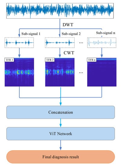
Figure 1.
Fault diagnosis scheme based on the proposed multi-information fusion ViT model.
2.1. DWT-Based Signal Decomposition
As described in Figure 1, to capture more fault-related information from small data samples to improve the diagnosis accuracy, the TFR maps of multiple different scale sub-signals are concatenated to input into the ViT model. In order to obtain the different scale sub-signals, DWT uses a set of base functions formed by wavelet scaling to decompose the original signal into different scale sub-signals with complete information in the pass frequency range [29]. Based on the concept of multiresolution analysis, the famous Mallat algorithm for wavelet decomposition and reconstruction is proposed by Mallat [30], which is described as follows.
Supposed that X is the time sequence of vibration signal x(t), and the orthogonal wavelet decomposition can be described by Equation (1):
where cj,k represents the scale coefficients, dj,k represents the wavelet coefficients, h and g are a pair of orthogonal mirror filter sets (QMF), j is the number of decomposition layers, and N is the data point number of the time sequence.
The wavelet reconstruction is the inverse of the wavelet decomposition, and the corresponding reconstruction equation is presented as Equation (2):
The multiresolution analysis property of a wavelet can decompose a signal at different scales with multiple resolutions, which can also decompose mixed signals consisting of various frequencies intertwined into different scale sub-signals to describe the characteristic information of the sub-signals of the different frequency bands. Figure 2 shows the results of a four-layer wavelet decomposition of an original signal to obtain an approximate signal A4 and a set of detailed signals, D1, D2, D3, and D4. Thus, the relationship between the decomposed sub-signals and the original signal X can be expressed as:
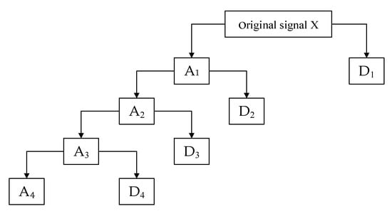
Figure 2.
DWT decomposition schematic. Ai indicates the ith layer approximate signal and Di represents the ith layer detailed signals.
2.2. CWT-Based Time–Frequency Representation Maps
The TFR maps of different scale sub-signals obtained by the time-frequency analysis method can reveal the relationship between the frequency components of the sub-signal and time, reflecting the vibration characteristic information of the signal. Considering that CWTs have good time–frequency localization capability and detect the singularity of the fault vibration signal, the CWT method was used to depict fault-related information from sub-signals in different frequency bands.
A basic function was translated and stretched to obtain Equation (4):
where τ and a are constants, and a > 0. When τ and a have different values, a cluster function can be obtained. When satisfies Equations (5)–(7), is referred to as the wavelet basis function.
where represents the Fourier transform of .
For any square integrable function , its continuous wavelet transform is defined by Equation (8):
where represents the energy finite space, a is the scale factor, representing the frequency-dependent scaling, and τ is the translational factor. a and τ determine the position of the wavelet window in the frequency and time domains. After the time-domain signal is transformed to obtain the scale domain, the signal scale received is converted into a TFR map using Equation (9):
where represents the centre frequency of the wavelet, is the sampling frequency of the signal, and is the actual frequency corresponding to scale a.
To make the transformed frequency sequence an equal difference sequence, the scale sequence take the following values:
where totalscal is the length of the scale sequence, which is set as 256. In addition, the actual frequency corresponding to the scale c/totalscal is fs/2. The value of the constant c can be calculated according to Equation (9), which can be obtained by the following equation:
Accordingly, the required scale sequence is obtained.
Generally, the wavelet basis function waveform selected should be similar to the fault characteristics of the signal [31]. Since the Morlet wavelet waveform is identical to the shock characteristics generated by bearing faults [32], the complex Morlet wavelet (cmor wavelet) has better adaptive performance. Here, the cmor wavelet function is adopted and given in Equation (12):
where is the bandwidth factor, and fc is the centre frequency factor.
2.3. ViT Model
The transformer network uses an acyclic network structure with parallel computation through an encoder–decoder and a self-attentive mechanism, drastically reducing the model training time [33]. Its structure is shown in Figure 3, which consists primarily of an embedding layer and a multilayer encoder–decoder. Each layer of the encoder consists of two sub-layers: a multiheaded attention layer and a feedforward connection layer. Each layer of the decoder consists of three sub-layers: a masked multiheaded attention layer, a multiheaded attention layer, and a feedforward connection layer. Each sub-layer is also followed by two sub-layers: a residual connection and layer normalisation. The transformer model is capable of long-range mining dependencies and parallel computation, and the local interactions do not limit this entirely self-attention-based mechanism of the transformer model. However, the transformer uses sequences as inputs, which is not directly applicable to two-dimensional images, and a transformer based on global information interactions tends to be computationally intensive and needs sufficient data samples.
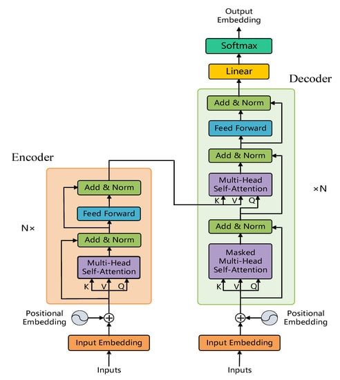
Figure 3.
Architecture of the transformer model.
Afterwards, the vision transformer (ViT) model for image classification tasks is proposed to solve these problems [11]. The ViT model consists of an embedding layer, an encoder, and a classifier, and its structure is shown in Figure 4. Firstly, the ViT model segments the input multilayer image into fixed-size image patches and flattens each image block into a sequence of image patches, and then performs a linear mapping of each image patch while adding position encoding to introduce the sequence position information, the images can retain their positional information. After, the new sequence of image patches is input into the transformer encoder, which is mainly composed of a multihead attention layer and a multilayer perceptron (MLP) layer; the multihead attention layer split the inputs into several heads so that each head can learn different levels of self-attention. Finally, the outputs of all the heads are concatenated and fed to the MLP head to obtain the classification results.
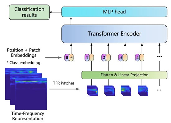
Figure 4.
Framework of the ViT model.
2.3.1. Embedding Layer
The ViT network firstly segments an image of size H × W × C into N = HW/P2 image patches of size P × P × C and then expands each patch into a one-dimensional vector to obtain . If d = N + 1 is the dimension of the ViT input vector space z0, the ViT model maps xp linearly and forms it into a d-dimensional vector space together with the category vectors, which is shown in Equation (13), as the input to the transformer encoder.
where is the learnable category vector, is the matrix for linear mapping, and is the location encoding information.
2.3.2. Position Encoding Module
Since the transformer framework does not contain recursive or convolutional operations, which is very important in time problems, to take full advantage of the location information, the ViT model introduces learnable location encoding Epos that extracts location information about image blocks through a learning process. The position encoding information is added together with the feature vector space and is sent to the encoder for feature information extraction. is a learnable matrix of dimensions [34].
2.3.3. Encoder
Figure 5a shows the internal structure of the ViT encoder, which consists of a stack of L identical layers for which the output of each layer serves as the input of the next layer. Each layer consists of two sub-layers: a multihead self-attention (MSA) layer and a multilayer perceptron (MLP) layer. The data are normalised using layer normalisation (LN) before entering each sub-layer and then are fused directly with the input for that sub-layer using residual joining after each sub-layer. Finally, after the L-layer network coding, the category vector is fed to the classifier to predict the image class. The computation process for the lth layer is expressed by Equations (14) and (15):
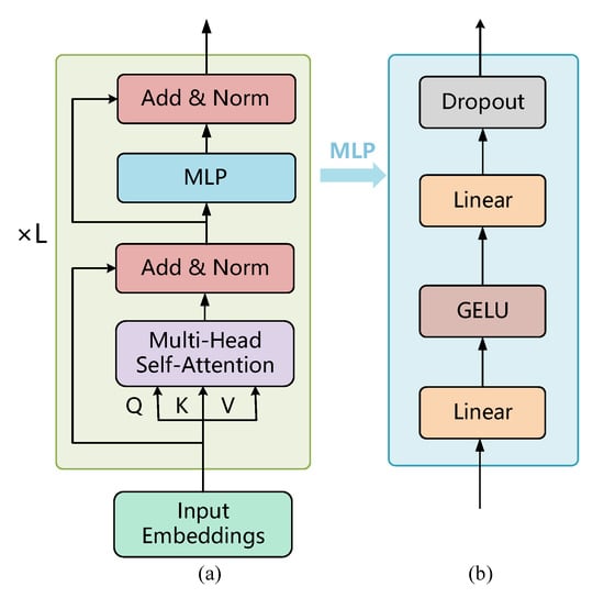
Figure 5.
(a) ViT encoder module and (b) internal structure of the MLP layer.
- Multihead self-attention layer
The transformer architecture solves the problem of limited convolutional kernel perceptual fields by introducing a self-attention mechanism to establish spatially long-range dependencies. The self-attention mechanism used by the ViT model is scaled dot product attention (SA), and its structure is shown in Figure 6. The scaled dot product attention is calculated using Equations (16) and (17):
where is the input sequence, which is projected through a linear mapping matrix UQKV to obtain three vectors: Q(Query), K(Key, and V(Value); h denotes the number of self-attentive heads; d/h is the output dimension of each self-attentive head; and dh is generally set to d/h to ensure that the number of model parameters remains unchanged when h is changed.
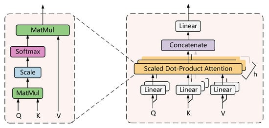
Figure 6.
Architecture of the multihead self-attention layer.
In addition, to improve the feature diversity and increase the expressiveness of the model, the ViT model uses a multihead self-attention mechanism. The multihead self-attentive layer uses multiple self-attentive heads for parallel computations; finally, the result is obtained by stitching the outputs of all the self-attentive heads together. The calculation process for the multihead attention is expressed by Equation (18):
where is the multiple attention weight matrix.
- MLP layer
The multilayer perceptron (MLP) is an extension of the single-layer perceptron, which can solve nonlinear problems that cannot be solved by the single-layer perceptron [35]. An MLP primarily consists of a fully connected layer and an activation function, and its structure is shown in Figure 5b. It is worth noting that ViT adds a dropout layer behind the fully connected layer of the MLP to improve the generalization ability of the network model. To improve the convergence speed of the network and avoid the gradient disappearance problem, the ViT model uses the Gaussian error linear units (GELU) activation function instead of the rectified linear unit (ReLU) activation function in the transformer network. The GELU activation function is calculated using Equation (19):
where x represents the input, and erf(•) denotes the Gaussian error function.
2.3.4. Classifier
The classifier serves to nonlinearly map the output of the encoder to obtain the final fault classification result. The classifier in the standard ViT model consists of a linear layer, a tanh activation function, and another linear layer. To reduce the computational effort, only one linear layer was used to form the classifier here. After the transformer encoder layer, the data are linearly transformed by the classifier to obtain a probability for each fault class, and the maximum value is taken as the final classified fault class y. The calculation process for the fault class classification is expressed by Equation (20):
2.3.5. Loss Function
The training process for the ViT model uses a general deep learning scheme with a stochastic gradient descent (SGD) algorithm to minimise the empirical risk. The loss function used by the ViT model is the cross-entropy (CE) loss function, which can be calculated using Equations (21) and (22):
where pi represents a sample class probability output sequence, c denotes the true class label of the sample, C denotes the number of labels of the sample, and N represents the number of training dataset samples [36].
3. Diagnosis Algorithm of the Multi-Information Fusion ViT Model
Figure 7 illustrates the fault diagnosis flow chart based on the multi-information fusion ViT model. Bearing vibration signals are divided into different data samples, which are divided into training dataset and testing dataset. The data samples in the training dataset are decomposed into sub-signals of different frequency bands by the DWT, and the corresponding TFR maps of the sub-signals can be obtained by CWTs. Then, these TFR maps of all the sub-signals are concatenated to train the ViT model. After, the TFR maps of the data sample in test dataset are concatenated to feed to the trained ViT model to obtain the diagnosis result.
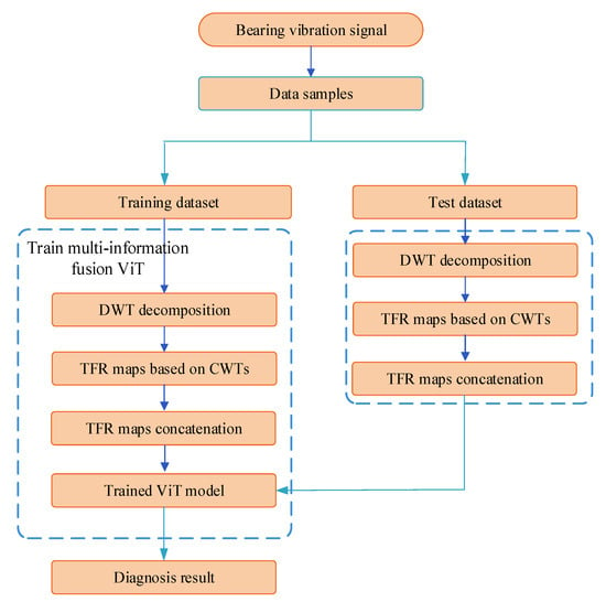
Figure 7.
Fault diagnosis process of the multi-information fusion ViT model.
4. Fault Diagnosis Analysis of Rolling Bearing
To verify the effectiveness of the multi-information fusion ViT model proposed in this paper, the Case Western Reserve University (CWRU) bearing vibration signals were used for the fault diagnosis experimental study [37]. Figure 8 shows the bearing fault test platform, primarily consisting of a motor, an acceleration sensor, a test bearing, and a dynamometer. A 6205-2RS JEM deep groove ball bearing was selected as the test bearing. Different bearing fault categories and damage levels were produced by the electric discharge machining (EDM) method. In addition, at the load of 0 HP and a spindle speed of 1797 r/min, drive-end bearing vibration signals were collected at a sampling frequency of 12 kHz.
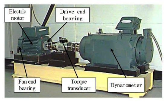
Figure 8.
Bearing fault test platform [37].
4.1. Dataset Description
In order to validate the diagnosis performance of the proposed multi-information fusion ViT model on small data samples, the fault diagnosis analysis was conducted using datasets of different sizes. Table 1 shows the detailed statistics for Dataset A, which contained a total of 10 bearing fault conditions, nine fault classes and one normal condition. The number of training data samples of each fault class was 100, the number of test data samples of each fault class was 60, and the total number of data samples for the training and test were 1000 and 600, respectively. In addition, there were 1024 data points in each data sample.

Table 1.
Detailed statistics of Dataset A.
4.2. Diagnosis Analysis
The original data samples were decomposed and transformed by DWT and CWT methods to obtain the TFRs maps for different scale sub-signals, such as four detailed signals, D1, D2, D3, and D4, and an approximate signal A4. The resolution of the TFRs was adjusted to a typical model input size, 224 × 224 × 3, using a dual cubic interpolation algorithm [38]. Figure 9 shows the one-dimensional detailed and approximate sub-signal and their corresponding TFRs maps, indicating that these different scale sub-signals exhibit different vibration characteristics in different frequency bands. Obviously, these detailed sub-signals and approximate sub-signal changes can be displayed from multiple angles through these TFRs, which can effectively describe the subtle fault characteristics of a sub-signal. These also demonstrate that different scale sub-signals can contain the different fault-related information. Thus, these TRFs of different scale sub-signals can be used as characteristic diagrams to characterise the fault conditions of bearings for fault diagnosis. Here, the TFR maps of the detailed signals D1, D2, D3, and D4 and an approximate signal A4 are concatenated to feed to the ViT model.
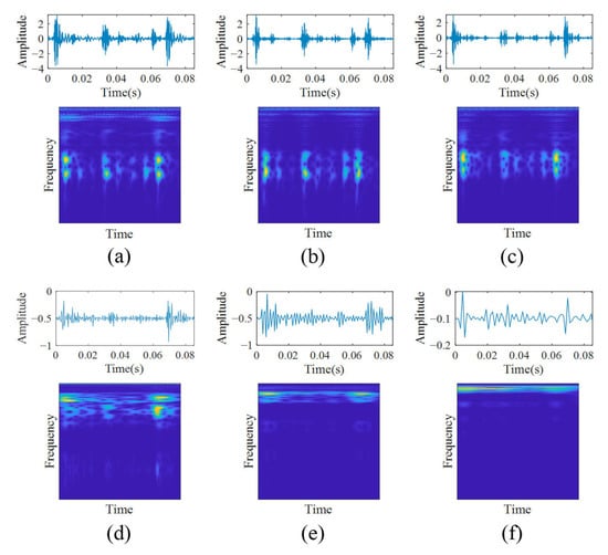
Figure 9.
Signal waveform and TFR map: (a) raw signal; (b) detailed signal D1; (c) detailed signal D2; (d) detailed signal D3; (e) detailed signal D4; (f) approximate signal A4.
To verify the effectiveness and superiority of the proposed multi-information fusion ViT model in this study, three others fault diagnosis models, such as the ViT model based on one-dimensional vibration signal (1D-ViT), ViT model based on the TFR of the original vibration signal, and a multi-information fusion CNN model based on the TFRs of different scale sub-signals, are also used for the fault diagnosis of bearings. The detailed model structures and hyperparameter settings of four fault diagnosis models are shown in Table 2 and Table 3.

Table 2.
Structure and hyperparameter selection for the multifeature fusion ViT model and two benchmark models.

Table 3.
Structure and hyperparameter selection for the multifeature fusion CNN model.
To test the stability of the diagnosis model, five-fold cross-validation tests were also conducted, the diagnosis accuracy statistics for the experimental results are listed in Table 4. Table 4 shows that the proposed multi-information fusion ViT model could achieve the highest diagnosis accuracy with 100%. Its lowest diagnosis accuracy and mean accuracy were 99.67% and 99.85%, respectively, and its highest diagnosis accuracy and lowest diagnosis and mean accuracy were the highest among the four diagnosis models. The highest diagnosis accuracy and lowest diagnosis and mean accuracy of the 1D-ViT model, at 89.33%, 86.17%, and 87.97%, respectively, were all the lowest among the four diagnosis models. In addition, the highest diagnosis accuracy and lowest diagnosis and mean accuracy of the ViT based on TFR was lower than that of the multi-information fusion CNN. These results indicate that the multi-information fusion ViT based on the TFRs of different scale sub-signals is superior to the multi-information fusion CNN and the 1D-ViT and ViT based on TFR. This is mainly because that the multi-information fusion ViT can extract more fault-related information from the TFRs of different scale sub-signals to improve the diagnosis accuracy, and the information fusion of all different scale sub-signals can improve the diagnosis accuracy. In addition, from Table 4 it can be seen that the difference between the highest diagnosis accuracy and lowest diagnosis accuracy of the multi-information fusion ViT model was only 0.33%, which was the lowest among all four diagnosis models. This also demonstrates that the multi-information fusion ViT model based on the TFRs of different scale sub-signals has strong stability because of the more fault-related information extraction from the different scale sub-signals.

Table 4.
Test results for the bearing dataset produced by the diagnostic models.
In addition, Figure 10 gives the confusion matrix of the highest and lowest diagnosis results of the proposed multi-information fusion ViT model, with accuracies of 100% and 99.67%, respectively. The columns represent the identified fault class labels, while the rows represent the true fault class labels for the different fault classes. Figure 10a show that each fault class of bearings were all identified with 100% accuracy, and Figure 10b displays that the diagnosis accuracy of each fault class of bearings was 100%, except for the medium rolling element fault. These experimental results also demonstrate that the proposed multi-information fusion ViT model can effectively identify all bearing fault classes further.
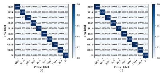
Figure 10.
Confusion matrix of (a) the best diagnosis result and (b) the worst diagnosis result for Dataset A produced by the multi-information fusion ViT model.
4.3. Diagnosis Generalization Analysis on Different Small Data Samples
In order to verify the diagnosis generalization of the proposed multi-information fusion ViT model on small data samples, five datasets (A, B, C, D, and E) with different numbers of training data samples were introduced for the diagnosis analysis. Thereinto, the total number of training samples for Datasets B, C, D, and E were 500, 240, 150, and 90, respectively, each dataset contained 600 test data samples, and the number of training data samples and test samples of each fault class in each dataset was the same. Figure 11 provides the diagnosis accuracy produced by the multi-information fusion ViT, the multi-information fusion CNN, and the 1D-ViT and ViT based on TFR on the Datasets A, B, C, D, and E. From Figure 11, it can be seen that the diagnosis accuracy of the multi-information fusion ViT were all the highest on these five datasets among these four diagnosis models. The diagnosis accuracy of the multi-information fusion ViT on these five datasets was higher than that of the ViT based on TFR, and the diagnosis accuracy of the 1D-ViT on these five datasets was the lowest among the four diagnosis models. All these indicate that the diagnosis generalization of the multi-information fusion ViT was superior to the other three diagnosis models even though the number of the training data samples was small. This was mainly because the multi-information fusion ViT can extract more fault-related information from the TFRs of different frequency band sub-signals.
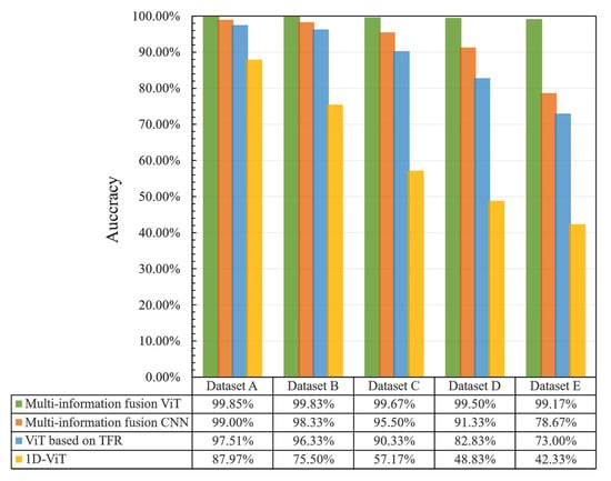
Figure 11.
Diagnosis accuracy for Datasets A, B, C, D, and E.
In addition, Figure 11 also shows that the diagnosis accuracy of these four diagnosis models decreased as the number of training samples decreased, but the diagnosis accuracy of the multi-information fusion ViT was still relatively high on the five datasets. Even though the total number of training data samples was 90, the diagnosis accuracy of the multi-information fusion ViT achieved 99.17%; this also demonstrates that the multi-information fusion ViT could diagnose the fault of bearings with the small data samples effectively and had a strong diagnosis generalization on the small data samples.
4.4. Anti-Noise Diagnosis Ability Analysis
To verify the diagnosis robustness of the proposed multi-information fusion ViT model, Gaussian white noise with a variety of signal-to-noise ratios (SNRs) was added to the data samples of Dataset A for fault diagnosis experiments [39]. The diagnosis results are shown in Figure 12. It can be seen that the proposed multi-information fusion ViT model could achieve the highest diagnosis accuracy on Dataset A with different SNRs, and the diagnosis accuracy of the 1D-ViT was the lowest among the four diagnosis models, the diagnosis accuracy of ViT based on TFR on Dataset A with different SNRs were all lower than that of the multi-information fusion CNN model. This is mainly because the TFR had a better noise suppression effect while characterizing more fault-related information compared with the one-dimensional vibration signal, and the multi-information fusion ViT model could extract more fault-related information from the TFRs of the different scale sub-signals and improve the anti-noise ability because of the multi-TRF maps fusion.
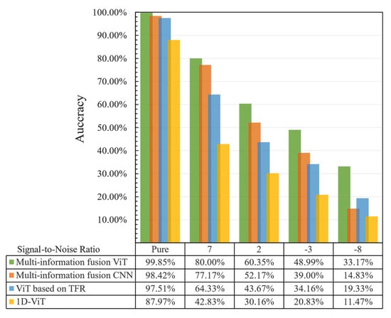
Figure 12.
Diagnostic accuracies of the different fault diagnosis methods at different signal-to-noise ratios.
Figure 12 also displays that the diagnosis accuracy of all these four methods decreased with the decreasing SNR. When the SNR was two, the diagnosis accuracy of the proposed multi-information fusion ViT model could achieve 60.35%, but the diagnosis accuracy of the other three diagnosis models was lower than 52.2%. In addition, when SNR was −8, the diagnosis accuracy of the proposed multi-information fusion ViT model is only 33.17%, but the diagnosis accuracy of the other three diagnosis models was lower than 20%. Obviously, even though the small data samples contained noise, the proposed multi-information fusion ViT model could diagnose the bearing fault effectively, and its anti-noise diagnosis ability was superior to the other three diagnosis models. This further demonstrates that the proposed multi-information fusion ViT model had strong robustness.
5. Conclusions
In this paper, a novel multi-information fusion ViT model based on the TFRs of different frequency band sub-signals was proposed to diagnose the bearing fault with the small data samples. In this method, the bearing vibration signal was decomposed into different scale sub-signals of s using DWTs firstly, and then the sub-signals were transformed into the TFRs by CWTs. Finally, the TFRs were concatenated to input to the ViT model to diagnose the bearing faults.
The effectiveness of the proposed multi-information fusion ViT model for the fault diagnosis of bearings with small data samples were verified by comparison with the multi-information fusion CNN and 1D-ViT and ViT based on TFR. At the same time, through a multifaceted comparison of the four methods on different small data samples and noisy data samples, the diagnosis results demonstrated that the proposed multi-information fusion ViT model had stronger generalization and robustness than the multi-information fusion CNN and 1D-ViT and ViT based on TFR for the fault diagnosis of bearings with small data samples. These results indicate that the multi-information fusion ViT model has promising prospects in the field of fault diagnosis with small data samples.
Author Contributions
Conceptualization, Z.X.; methodology, X.T. and Z.X.; software, X.T. and Z.X.; validation, Z.X. and Z.W.; formal analysis, X.T.; investigation, X.T. and Z.X.; data curation, X.T.; writing—original draft preparation, X.T. and Z.X.; writing—review and editing, X.T. and Z.X.; visualization, X.T.; supervision, Z.W.; project administration, Z.X.; funding acquisition, Z.X. All authors have read and agreed to the published version of the manuscript.
Funding
This research was funded by the National Natural Science Foundation of China (Grant No. 51775391), the Open Research Foundation of State Key Lab. of Digital Manufacturing Equipment & Technology in the Huazhong University of Science & Technology (Grant No. DMETK F2017010).
Data Availability Statement
The data that were used to support this study are available at the Case Western Reserve University Bearing Data Center [37].
Conflicts of Interest
The authors declare no conflict of interest.
References
- Upadhyay, R.K.; Kumaraswamidhas, L.A.; Azam, M.S. Rolling element bearing failure analysis: A case study. Case Stud. Eng. Fail. Anal. 2013, 1, 15–17. [Google Scholar] [CrossRef]
- Zhao, X.; Jia, M.; Bin, J.; Wang, T.; Liu, Z. Multiple-Order Graphical Deep Extreme Learning Machine for Unsupervised Fault Diagnosis of Rolling Bearing. IEEE Trans. Instrum. Meas. 2020, 70, 3506012. [Google Scholar] [CrossRef]
- Yan, X.; Jia, M. A novel optimized SVM classification algorithm with multi-domain feature and its application to fault diagnosis of rolling bearing. Neurocomputing 2018, 313, 47–64. [Google Scholar] [CrossRef]
- Shao, H.; Jiang, H.; Zhao, H.; Wang, F. A novel deep autoencoder feature learning method for rotating machinery fault diagnosis. Mech. Syst. Signal Process. 2017, 95, 187–204. [Google Scholar] [CrossRef]
- Zhang, H.; Wang, R.; Pan, R.; Pan, H. Imbalanced Fault Diagnosis of Rolling Bearing Using Enhanced Generative Adversarial Networks. IEEE Access 2020, 8, 185950–185963. [Google Scholar] [CrossRef]
- Hoang, D.-T.; Kang, H.-J. A survey on Deep Learning based bearing fault diagnosis. Neurocomputing 2019, 335, 327–335. [Google Scholar] [CrossRef]
- Zhang, S.; Zhang, S.; Wang, B.; Habetler, T.G. Deep learning algorithms for bearing fault diagnostics—A comprehensive review. IEEE Access 2020, 8, 29857–29881. [Google Scholar] [CrossRef]
- Fuan, W.; Hongkai, J.; Haidong, S.; Wenjing, D.; Shuaipeng, W. An adaptive deep convolutional neural network for rolling bearing fault diagnosis. Meas. Sci. Technol. 2017, 28, 095005. [Google Scholar] [CrossRef]
- Touvron, H.; Cord, M.; Douze, M.; Massa, F.; Sablayrolles, A.; Jégou, H. Training data-efficient image transformers & distillation through attention//International Conference on Machine Learning. PMLR 2021, 139, 10347–10357. [Google Scholar]
- Vaswani, A.; Shazeer, N.; Parmar, N.; Uszkoreit, J.; Jones, L.; Gomez, A.N.; Kaiser, Ł.; Polosukhin, I. attention is all you need. Adv. Neural Inf. Process. Syst. 2017, 30, 5998–6008. [Google Scholar]
- Dosovitskiy, A.; Beyer, L.; Kolesnikov, A.; Weissenborn, D.; Zhai, X.; Unterthiner, T.; Dehghani, M.; Minderer, M.; Heigold, G.; Gelly, S.; et al. An Image is Worth 16x16 Words: Transformers for Image Recognition at Scale. In Proceedings of the International Conference on Learning Representations, Virtual Conference, 26 April–1 May 2020. [Google Scholar]
- Yuan, L.; Chen, Y.; Wang, T.; Yu, W.; Shi, Y.; Jiang, Z.; Tay, F.E.H.; Feng, J.; Yan, S. Tokens-to-Token Vit: Training Vision Transformers from Scratch on Imagenet. In Proceedings of the IEEE/CVF International Conference on Computer Vision, Montreal, QC, Canada, 10–17 October 2021; pp. 558–567. [Google Scholar]
- Ding, Y.; Jia, M.; Miao, Q.; Cao, Y. A novel time–frequency Transformer based on self–attention mechanism and its application in fault diagnosis of rolling bearings. Mech. Syst. Signal Process. 2022, 168, 108616. [Google Scholar] [CrossRef]
- Zhou, K.; Diehl, E.; Tang, J. Deep convolutional generative adversarial network with semi-supervised learning enabled physics elucidation for extended gear fault diagnosis under data limitations. Mech. Syst. Signal Process. 2023, 185, 109772. [Google Scholar] [CrossRef]
- Luo, J.; Huang, J.; Ma, J.; Li, H. An evaluation method of conditional deep convolutional generative adversarial networks for mechanical fault diagnosis. J. Vib. Control. 2021, 28, 1379–1389. [Google Scholar] [CrossRef]
- Arjovsky, M.; Chintala, S.; Bottou, L. Wasserstein generative adversarial networks//International conference on machine learning. PMLR 2017, 70, 214–223. [Google Scholar]
- Yang, J.; Liu, J.; Xie, J.; Wang, C.; Ding, T. Conditional GAN and 2-D CNN for Bearing Fault Diagnosis with Small Samples. IEEE Trans. Instrum. Meas. 2021, 70, 3525712. [Google Scholar] [CrossRef]
- Yan, R.; Shen, F.; Sun, C.; Chen, X. Knowledge Transfer for Rotary Machine Fault Diagnosis. IEEE Sensors J. 2019, 20, 8374–8393. [Google Scholar] [CrossRef]
- He, Z.Y.; Shao, H.D.; Wang, P.; Janet, L.; Cheng, J.S.; Yang, Y. Deep transfer multi-wavelet auto-encoder for intelligent fault diagnosis of gearbox with few target training samples. Knowl. Based Syst. 2020, 191, 105313. [Google Scholar] [CrossRef]
- Chen, W.; Qiu, Y.; Feng, Y.; Li, Y.; Kusiak, A. Diagnosis of wind turbine faults with transfer learning algorithms. Renew. Energy 2020, 163, 2053–2067. [Google Scholar] [CrossRef]
- Cao, P.; Zhang, S.; Tang, J. Preprocessing-free gear fault diagnosis using small datasets with deep convolutional neural network-based transfer learning. IEEE Access 2018, 6, 26241–26253. [Google Scholar] [CrossRef]
- Li, X.; Jiang, H.; Niu, M.; Wang, R. An enhanced selective ensemble deep learning method for rolling bearing fault diagnosis with beetle antennae search algorithm. Mech. Syst. Signal Process. 2020, 142, 106752. [Google Scholar] [CrossRef]
- Zhang, Y.; Wang, J.; Zhang, F.; Lv, S.; Zhang, L.; Jiang, M.; Sui, Q. Intelligent fault diagnosis of rolling bearing using the ensemble self-taught learning convolutional auto-encoders. IET Sci. Meas. Technol. 2022, 16, 130–147. [Google Scholar] [CrossRef]
- Hoang, D.T.; Tran, X.T.; Van, M.; Kang, H.J. A Deep Neural Network-Based Feature Fusion for Bearing Fault Diagnosis. Sensors 2021, 21, 244. [Google Scholar] [CrossRef] [PubMed]
- Xia, M.; Li, T.; Xu, L.; Liu, L.; De Silva, C.W. Fault diagnosis for rotating machinery using multiple sensors and convolutional neural networks. IEEE/ASME Trans. Mechatron. 2017, 99, 101–110. [Google Scholar] [CrossRef]
- Silik, A.; Noori, M.; Altabey, W.A.; Ghiasi, R.; Wu, Z. Comparative Analysis of Wavelet Transform for Time-Frequency Analysis and Transient Localization in Structural Health Monitoring. Struct. Durab. Heal. Monit. 2021, 15, 1–22. [Google Scholar] [CrossRef]
- Zhang, J.; Feng, F.; Marti-Puig, P.; Caiafa, C.F.; Sun, Z.; Duan, F.; Solé-Casals, J. Serial-EMD: Fast empirical mode decomposition method for multi-dimensional signals based on serialization. Inf. Sci. 2021, 581, 215–232. [Google Scholar] [CrossRef]
- Chaovalit, P.; Gangopadhyay, A.; Karabatis, G.; Chen, Z. Discrete wavelet transform-based time series analysis and mining. ACM Comput. Surv. 2011, 43, 1–37. [Google Scholar] [CrossRef]
- Morlet, J. Seismic tomorrow: Interferometry and quantum mechanics//Geophysics. SOC Explor. Geophys. 1976, 41, 366. [Google Scholar]
- Mallat, S.G. A theory for multi-resolution signal decomposition: The wavelet representation. IEEE Trans. Pattern Anal. Mach. Intell. 1989, 11, 674–693. [Google Scholar] [CrossRef]
- Kankar, P.K.; Sharma, S.C.; Harsha, S.P. Fault diagnosis of ball bearings using continuous wavelet transform. Appl. Soft Comput. 2011, 11, 2300–2312. [Google Scholar] [CrossRef]
- Chen, Z.; Cen, J.; Xiong, J. Rolling Bearing Fault Diagnosis Using Time-Frequency Analysis and Deep Transfer Convolutional Neural Network. IEEE Access 2020, 8, 150248–150261. [Google Scholar] [CrossRef]
- Gehring, J.; Auli, M.; Grangier, D.; Yarats, D.; Dauphin, Y.N. Convolutional sequence to sequence learning//International conference on machine learning. PMLR 2017, 70, 1243–1252. [Google Scholar]
- Carion, N.; Massa, F.; Synnaeve, G.; Usunier, N.; Kirillov, A.; Zagoruyko, S. End-to-End Object Detection with Transformers. In Proceedings of the European Conference on Computer Vision, Glasglow, Scotland, 23–28 August 2020; pp. 213–229. [Google Scholar]
- Taud, H.; Mas, J.F. Multilayer Perceptron (MLP). In Geomatic Approaches for Modeling Land Change Scenarios; Springer: Cham, Switzerland, 2018; pp. 451–455. [Google Scholar]
- Srivastava, N.; Hinton, G.; Krizhevsky, A.; Sutskever, I.; Salakhutdinov, R. Dropout: A simple way to prevent neural networks from overfitting. J. Mach. Learn. Res. 2014, 15, 1929–1958. [Google Scholar]
- The Case Western Reserve University Bearing Data Center. Bearing Data Center Fault Test Data. 1998. Available online: http://csegroups.case.edu/bearingdatacenter/pages/download-data-file (accessed on 23 January 2021).
- Keys, R. Cubic convolution interpolation for digital image processing. IEEE Trans. Acoust. Speech Signal Process. 1981, 29, 1153–1160. [Google Scholar] [CrossRef]
- Hebda-Sobkowicz, J.; Zimroz, R.; Wyłomańska, A. Selection of the Informative Frequency Band in a Bearing Fault Diagnosis in the Presence of Non-Gaussian Noise—Comparison of Recently Developed Methods. Appl. Sci. 2020, 10, 2657. [Google Scholar] [CrossRef]
Disclaimer/Publisher’s Note: The statements, opinions and data contained in all publications are solely those of the individual author(s) and contributor(s) and not of MDPI and/or the editor(s). MDPI and/or the editor(s) disclaim responsibility for any injury to people or property resulting from any ideas, methods, instructions or products referred to in the content. |
© 2023 by the authors. Licensee MDPI, Basel, Switzerland. This article is an open access article distributed under the terms and conditions of the Creative Commons Attribution (CC BY) license (https://creativecommons.org/licenses/by/4.0/).