A Dynamic Self-Attention-Based Fault Diagnosis Method for Belt Conveyor Idlers

Abstract

Idlers are typical rotating parts of a belt conveyor carrying the conveyor belt and materials. The complex operating noise and unstable features lead to poor accuracy of sound-based idler fault diagnosis. This paper proposes a fault diagnosis method for belt conveyor idlers based on Transformer’s dynamic self-attention (DSA). Firstly, the A-weighted time-frequency spectrum of the idler sound is extracted as the input. Secondly, based on the DSA block, the multi-frequency cross-correlation DSA algorithm is designed to extract the cross-correlation features between different frequency bands in the input feature map, and the global DSA algorithm is applied to perceive and enhance the global correlation features in parallel. Finally, the cross-correlation and global correlation features are concatenated and linearly projected into a fault-type space to diagnose typical bearing and roller faults of idlers. The method makes full use of the relevant information scattered in different frequency bands of the idler running sound under complex working conditions and reduces the negative effect of the strong running noise on the extraction of weak fault features. Experimental results show that the fault diagnosis accuracy is 94.6% and the latency is 27.8 ms.

1. Introduction

Belt conveyors are continuous transportation equipment in modern production. Featured with large transportation capacity, long distance, low freight, and high efficiency, belt conveyors have been widely used in the coal industry, mines, ports, electric power, metallurgy, chemical industry, and other fields [1,2]. Idlers are the key components of a belt conveyor carrying the conveyor belt and materials. Due to poor lubrication, fatigue, foreign debris intrusion of the bearing, uneven load, or heavy impact on the roller, etc. [3], the idlers suffer from abnormal vibration and noise, damage, fracture, jamming, and other faults, resulting in increased transportation energy consumption and serious accidents, such as deviation, tearing, and fire of the conveyor belt. Due to the large number, scattered distribution, and complex working conditions of idlers, diagnosing faults of idlers by using their running sound appears to be an efficient approach. However, the strong running noise of belt conveyors will submerge the running sound of idlers, which seriously reduces accuracy and reliability, posing a severe challenge to the fault diagnosis method.

Recent successes in artificial intelligence have promoted and significantly increased the use of machine-learning and deep-learning technologies in the fault detection and diagnosis of belt conveyors. In terms of idler fault diagnosis, Muralidharana et al. present an idler fault diagnosis method based on a decision tree (DT) algorithm, which uses the statistical metrics of idler vibration signals to train the DT-based fault diagnosis model, and the experimental results show a good performance in the classification of four types of idler faults [4]. Ravikumar et al. propose an idler fault diagnosis method based on the K-star algorithm, which uses the time-domain features of idler vibration signals as the input of the K-star algorithm and achieves better idler fault classification results [5]. Peng et al. propose an idler fault diagnosis method based on convolutional neural networks (CNN), where the CNN is trained by using the wavelet packet decomposition features extracted from idler sound signals, and this method achieves accurate and robust idler fault diagnosis [6]. Yang et al. present an idler fault diagnosis method based on deep convolutional neural networks (DCNN), which uses Mel frequency cepstrum coefficients (MFCC) of idler sound signals as the input to train the DCNN, and compared with support vector machine (SVM) and CNN, this method shows more accurate results in the prediction of idler fault degree [7]. Liu et al. propose a method for idler fault diagnosis based on machine learning, where the MFCC of idler sound signals is also used as the input to train the gradient boosting decision trees (GBDT) in fault classification, and the experimental results show that this method achieves a diagnostic accuracy of 94.53% on the test set [8]. In the aspects of conveyor belt fault detection, Qu et al. propose a conveyor belt damage detection method based on adaptive depth convolution networks, which realizes faster and more reliable conveyor belt damage detection than SVM [9]. Mao et al. present a defect classification algorithm for steel cord conveyor belt defects based on improved skewness decision tree SVM [10]. Che et al. propose a longitudinal tear detection method for conveyor belts based on SVM, which uses the audio and video features of longitudinal tearing to train SVM, and this method achieves more accurate detection results than K-nearest neighbors and random forest (RF) algorithms [11]. Meanwhile, machine-learning and deep-learning technologies are becoming increasingly pervasive as a means of improving the accuracy and robustness of the conveyor belt deviation fault detection [2,12], conveyor belt speed measurement [13], and positioning of inspection devices for belt conveyors [14] in a complex environment. With loud running and environmental noise in the working scene of belt conveyors, the energy of the interference part in the collected sound or vibration signal is much stronger than the useful signal. Extracting inconspicuous useful features from the chaotic signal is the key challenge to the fault diagnosis algorithm.

Idlers are typical rotating machinery. In recent years data-driven machine-learning and deep-learning algorithms have consolidated their leading position in the fault diagnosis of rotating machinery [15,16]. Zhang et al. propose a bearing fault diagnosis method based on SVM: by determining the search interval and optimal parameter combination in the feature space, the SVM classification model is optimized to improve the accuracy of fault diagnosis [17]. Jiang et al. propose a fault degree identification method for wind turbine gearboxes based on multiscale convolutional neural networks (MSCNN), which is used to extract multiscale and complementary high-level fault features and classify faults, and this method achieves better identification results than traditional CNNs [18]. Li et al. propose a rotating machinery fault diagnosis method based on deep-transfer learning, which transfers the diagnostic knowledge learned from the sufficient supervision data of multiple rotating machines to the target equipment through domain adversarial training, to improve the fault diagnostic accuracy of rotating machinery under weak supervision [19]. Xing et al. propose a gear fault diagnosis method based on deep-belief networks. Aiming at the problem of feature distributions changing under new working conditions, the distribution-invariant deep-belief network is used to learn distribution-invariant features directly from raw vibration data, to improve the accuracy of gear fault diagnosis under varying working conditions [20]. Aiming at the same problem under new working conditions, Moshrefzadeh et al. propose a bearing fault diagnosis method based on subspace k-nearest neighbors (S-KNN), using spectral amplitude modulation and improved kurtosis of the modified signal’s squared envelope spectrum algorithms to decompose the vibration signals and extract features and train the S-KNN model using the obtained feature vectors. The experimental results show that the classification result of S-KNN based on the features is better than that of SVM [21]. As for the machine-learning-based algorithms, the performance of feature-extraction algorithms has a significant impact on their diagnosis results, and as for the deep-learning-based algorithms, which combine feature extraction and classification to achieve end-to-end fault diagnosis, network architectures, and data sets are the key points, and as the network cannot run in parallel in the depth direction, a deeper network suffers from a longer inference latency.

In 2017, Google proposed a sequence prediction network based on a self-attention mechanism called Transformer [22], which is outstanding in natural language processing. In 2020, Facebook successfully introduced the transformer structure into machine vision. This network detects the target in parallel using the correlation between the target and the whole image content, and it outperforms the CNN baseline Faster RCNN [23]. Since then, Transformer has rapidly emerged in machine vision tasks such as low-level computer vision [24], object detection [25], video question answering [26], image quality evaluation [27], etc. Different from CNNs focusing on local features [28], Transformer uses the dynamic self-attention mechanism to establish the global correlation between elements in the sequence, so it focuses on the global features [25]. To extract the periodic or constant broadband weak features from signals with strong noise interference, a global feature perception way is more suitable than a local one. The idler sound signal is submerged by strong energy noise, and the fault features are correlated by the time and frequency axes of its time-frequency domain (TFD) feature map [29]. Using CNNs to perceive the global fault features requires a deep network, while Transformer can achieve better performance by using a much shallower one. Using Transformer’s DSA mechanism to extract multi-frequency cross-correlation (MF-Cov) features from the TFD feature map of faulty idler sound, as well as perceive and enhance the global correlation features, will facilitate improvements in the accuracy of the idler fault diagnosis algorithm under strong noise background.

In order to improve the accuracy and reliability of the sound-based idler fault diagnosis method under strong noise, an idler fault diagnosis method based on DSA is proposed in this paper. The A-weighted TFD feature map of the idler running sound is used as the input, then based on Transformer’s DSA, the MF-Cov DSA algorithm is designed to extract the cross-correlation features between different bands in the input feature map, and the global DSA algorithm is applied to perceive and enhance the global correlation features in parallel. Then both features are concatenated and linearly projected into the low dimensional fault type space to realize fault diagnosis.

The rest of this paper is organized as follows. Section 2 presents the sound feature analysis of faulty idlers. and provides a de-tailed description of the proposed method. The experimental results and analysis are presented in Section 3. The conclusions are stated in Section 4.

2. Materials and Methods

2.1. Sound Feature Analysis of Faulty Idlers

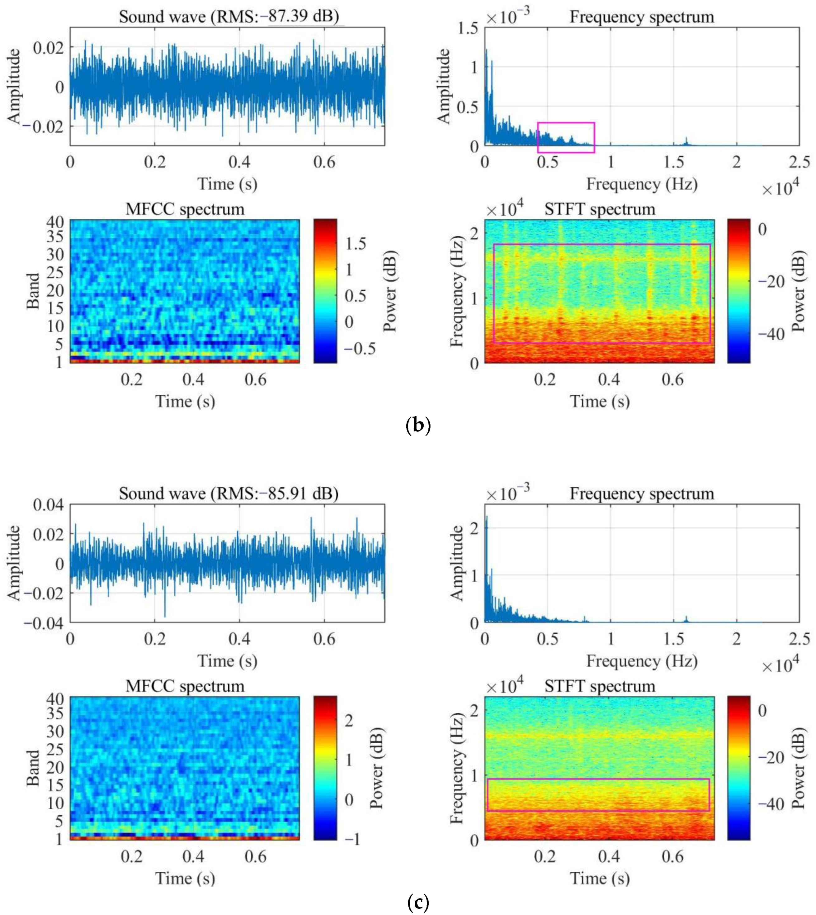
Idler faults are divided into bearing faults and roller faults, which are mainly characterized by multi-frequency cross-correlation and global correlation on the time-frequency spectrum. Ideally, for the intact idler, there should be no noise in the middle- and high-frequency bands of the time-frequency spectrum of the running sound. When an idler bearing fails, the fault point will be periodically collided or rubbed, resulting in the middle- and high-frequency abnormal sound modulated by a specific frequency range of periodic pulse or dynamic waveform. Obvious side frequency will appear in the Fourier spectrum, and periodic fringes will also appear in the time-frequency spectrum, that is, if the inner ring, outer ring, or rolling element of the bearing fails, according to the number, size, contact angle, and other parameters of the rolling element, the fault characteristic frequency (the envelope period of the specific frequency band sound emitted by the faulty idler, i.e., ball pass frequency outer race, ball pass frequency inner race, ball spin frequency, etc.) has specific multiple relationships with the rotation frequency, so the side frequency and fringe appear in the carrier frequency band (i.e., the middle- and high-frequency band), and the difference between the side and carrier frequencies or the frequency of the fringe is the fault characteristic frequency. When the idler is jammed, the continuous friction between the idler roller and conveyor belt will emit an inconspicuous friction sound, and its energy is evenly distributed in a wide frequency range. However, in real working conditions, as shown in Figure 1, due to the strong energy and broadband running noise emitted by the driving components, conveyor belts, adjacent idlers, and anti-slanting rollers, and by the frame resonance, for the intact idler, the middle- and high-frequency of its running sound contains noise, as shown in the rectangular boxes of Figure 1a. For the idler with bearing faults, its weak sound is submerged by the strong running noise of the belt conveyor, resulting in imperceptible changes in the sound intensity, and the side frequency on the Fourier spectrum is not significant, and the period of the fringe on the time-frequency spectrum is unstable due to the change of bearing radial force and insufficient lubrication, as shown in the rectangular boxes of Figure 1b. After the idler is jammed, the broadband energy in the frequency spectrum overlaps with the middle- and low-frequency operation noise, as shown in the rectangular boxes of Figure 1c. The low-frequency part of the time-frequency spectrum has strong running noise and modulation wave with the same frequency as the rotation speed, and the latter is strongly related to the fault characteristic frequency, that is, the multi-frequency cross-correlation feature. The frequency spectrum of the roller friction sound and the conveyor running noise overlap, and the energy in the overlapped part has a wide distribution range, that is, the global correlation feature.

From the short-time Fourier transform (STFT) spectrum, it can be seen that the low-frequency (0–5 kHz) running noise always exists and longitudinal stripes show up in the STFT spectrum of the bearing fault in Figure 1b, and different bearing faults (i.e., inner ring, outer ring, and rolling element faults) show different stripe spacing. However, the stripe strength and spacing of the same fault are not uniform because the rolling elements rotate randomly, and the force at the fault point changes dynamically during rotation. When the idler is jammed, the friction sound appears as a uniform energy band in the middle-frequency band of the STFT spectrum, which is different from that of the intact state. Since Mel frequency cepstral (MFC) makes a weighted sum of the energy of specific frequency bands in the STFT spectrum, the above-mentioned features are not salient. These features are widely distributed along the time and frequency axes of the TFD spectrum in different forms, so it is hard to diagnose these faults accurately by using the traditional feature extraction and fault classification methods. The requirement for a fault diagnosis algorithm is to be able to extract rotation frequency and fault characteristic frequency information, perceive and synthesize global features, intelligently extract discriminant features, and overcome the interference of strong running noise.

2.2. Dynamic Self-Attention-Based Idler Fault Diagnosis Method

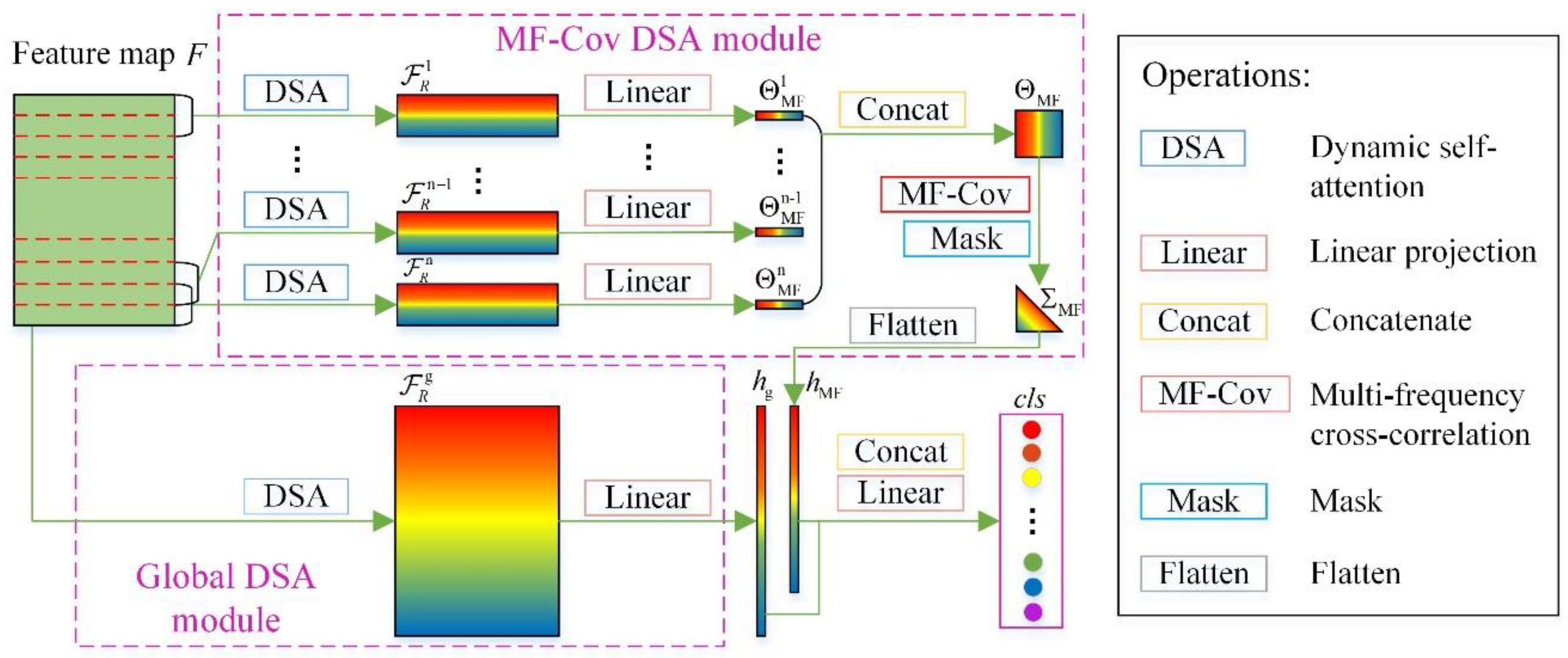
The proposed method is shown in Figure 2: the collected idler running sound is preprocessed in TFD to obtain the feature map, which is the input to the idler fault diagnosis model based on DSA to obtain the fault prediction label. In the training stage, samples in the training set are used as input, and the cross-entropy loss function is used to calculate the loss of predicted labels and true labels and then to optimize the model parameters. In the test stage, samples in the test set are used as input, and the output predicted label is the diagnosis result.

For the extraction and enhancement of the rotation frequency, fault characteristic frequency and global correlation information, and the classification of different faults, we propose the fault diagnosis model based on the DSA unit of Transformer, which includes two parallel intelligent information processing branches, namely, MF-Cov DSA module and global DSA module, aimed at dealing with the periodic bearing faults and globally related idler jamming faults, respectively. After the output of the two modules is concatenated, the predicted label is obtained through linear projection.

2.3. Time-Frequency Domain Feature Extraction and Preprocessing Method

The distribution of carrier and modulation frequencies along the time axis can indicate different idler faults. Due to the strong running noise, paying too much attention to the instantaneous frequency will lead to poor robustness of the extracted features. Therefore, the Fourier transform-based features such as MFCC and STFT spectrums are more robust and intuitive than the spectrums of Hilbert Huang transform and wavelet transform. Both MFC and STFT need to frame and window the signals, and then perform fast Fourier transform (FFT) on each frame. Different from STFT, MFC uses a set of triangular windows to obtain the weighted sum for the power spectrum of each frame and then uses discrete cosine transform to obtain the feature coefficients. MFC compresses and transforms the STFT spectrum along the frequency axis to get more concise and representative features. It is dedicated to speech feature extraction and compresses the amount of information as much as possible while maintaining speech intelligibility. In addition, it pays more attention to medium- and low-frequency sound and combines broadband information, which will inevitably lead to the loss of useful features, especially in the sound feature extraction of rotating machinery.

STFT spectrum is the most original TFD feature of the idler running sound as it contains a large number of broadband noises that pollute the spectrum of faulty idler sound. However, arbitrary band filtering may damage the useful features. Therefore, we propose a method to preprocess the STFT spectrum using the acoustic gain curve. According to the characteristics of mechanical fault sound and running noise, A-weighting or C-weighting can be used to maintain or enhance the useful frequency components on the STFT spectrum, and attenuate or eliminate the irrelevant frequency components, which can improve the signal-to-noise ratio (SNR) of TFD feature map. Given the STFT spectrum of a sound sample $S=\left[S_1 S_2\dots S_{\mathrm{T}}\right]$, T is the frame number,$S_i \left(i=1,2,\dots ,\mathrm{T}\right)$ is the frequency spectrum of each frame, each spectral line of the weighted STFT spectrum $\tilde{S}$ can be expressed as:

$${\tilde{S}}_i=S_i\odot {\psi }_x, i=1,2,\dots ,\mathrm{T}$$

(1)

where $\odot$ represents element product, $x$ can be A or C, ${\psi }_A$ and ${\psi }_C$ represent the weight vectors of A-weighting and C-weighting. The elements of ${\psi }_A$ can be determined by:

$${\psi }_A\left(f\right)=\frac{{10}^{-A_{1000}/20}{f}_4^2{f}^4}{\left(f^2+f_1^2\right){\left(f^2+f_2^2\right)}^{0.5}{\left(f^2+f_3^2\right)}^{0.5}\left(f^2+f_4^2\right)}$$

(2)

where $f$ is the frequency, $A_{1000}$ = −2.000 dB is a constant expressed in decibels, which provides an amplitude gain of 0 dB frequency weighting at $f$ = 1000 Hz, $f_1$ = 20.6 Hz, $f_2$ = 107.7 Hz, $f_3$ = 737.9 Hz, $f_4$ = 12,194 Hz [30]. The elements of ${\psi }_C$ can be determined by:

$${\psi }_C\left(f\right)=\frac{{10}^{-C_{1000}/20}{f}_4^2{f}^4}{\left(f^2+f_1^2\right)\left(f^2+f_4^2\right)}$$

(3)

where $C_{1000}$ = −0.062 dB is a constant providing an amplitude gain of 0 dB frequency weighting at $f$ = 1000 Hz. Figure 3 shows the gain curves of A-weighting and C-weighting. It can be seen that A-weighting enhances the frequency components in the range of 1–10 KHz, eliminates the components below 20 Hz, and other frequency components, while C-weighting retains most of the audible sound and does not enhance the components of mechanical fault sound.

2.4. Idler Fault Diagnosis Model Based on Dynamic Self-Attention

Figure 4 illustrates the proposed idler fault diagnosis model based on DSA, the preprocessed TFD feature map $\tilde{S}$ is taken as the input $F$, and it is sent to MF-Cov DSA module and global DSA module in parallel, then advanced MF-Cov feature vector $h_{\mathrm{MF}}$ and global correlation feature vector $h_{\mathrm{g}}$ can be obtained. Both features are concatenated and linearly projected into the fault-type space to realize fault diagnosis. MF-Cov DSA module and global DSA module are the main feature extraction modules, both are based on the DSA block of Transformer.

2.4.1. Dynamic Self-Attention

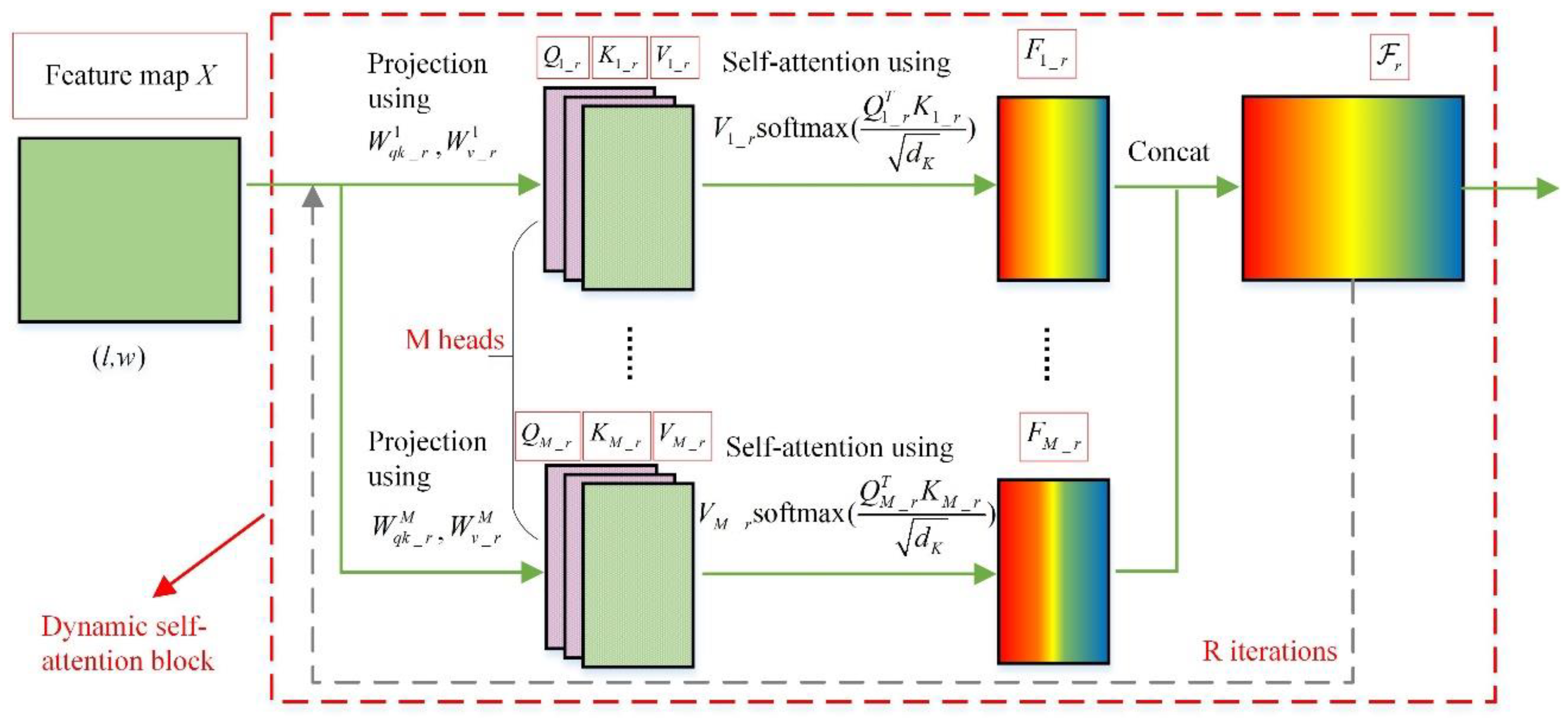
The standard or visual Transformer uses a DSA-based module to encode and decode the positional encoded input, then the decoder outputs the final detection results. DSA uses $M$ groups of projection matrices to map the input to $M$ groups of query/key/value embeddings, which are the feature maps focusing on different parts. The dimension length of each embedding is reduced to 1/$M$, and the self-attention operation is carried out for each group of embeddings, that is, the multi-head self-attention operation. Then, the obtained results are concatenated along feature axis and taken as the input of next iteration. The output of DSA is obtained after $R$ iterations, with the same size as the input [22], and its structure is presented in Figure 5.

Firstly, the learnable projection matrices $W_{qk\_r}^i$, $W_{v\_r}^i$ $\left(i=1,2,\dots , M\right)$ are used to project the input feature $X$ with size (l, w) into a low dimensional feature space to obtain $M$ groups of query/key/value embeddings:

$$\begin{gathered} Q_{i\_r},K_{i\_r}=X{W}_{qk\_r}^i, i=1,2,\dots , M \\ V_{i\_r}=X{W}_{v\_r}^i, i=1,2,\dots , M \end{gathered}$$

(4)

where $r$, $l$ and $w$ are the index of iterations, the length of time sequence, and the length of feature dimension, respectively. The query/key embeddings of each head share the same projection matrix to reduce the number of parameters, overfitting risk, and training difficulty of the model. In the low dimensional feature space, the length of time dimension remains unchanged, and the length of feature dimension is reduced to $1/M$. Each element of the same dimension is connected to all elements at that time through the same column of the learnable projection matrix, and has a global receptive field at that time. The establishment of such global connections is conducive to the intelligent identification of fault features and common noise in the input, so that the useful features are not submerged by strong running noise.

Secondly, the multi-head self-attention operation is conducted to get $M$ high-level feature maps:

$$F_{i\_r}=V_{i\_r}softmax\left(\frac{Q_{i\_r}^T{K}_{i\_r}}{\sqrt{d_K}}\right), i=1,2,\dots , M$$

(5)

where $d_K$ is the dimension length of key embeddings. $\mathrm{Softmax}(·)$ maps vector entries between $\left(0, 1\right)$. For a 2-dimensional matrix $A$ with size $\left(d,d\right)$, the operation will be conducted on the last dimension:

$$softmax\left(A\right)=\left[\begin{array}{ccc}\frac{e^{A_{11}}}{{{\displaystyle \sum }}_{j=1}^d{e}^{A_{1j}}}& \cdots & \frac{e^{A_{1d}}}{{{\displaystyle \sum }}_{j=1}^d{e}^{A_{1j}}}\\ ⋮& \ddots & ⋮\\ \frac{e^{A_{d1}}}{{{\displaystyle \sum }}_{j=1}^d{e}^{A_{dj}}}& \cdots & \frac{e^{A_{dd}}}{{{\displaystyle \sum }}_{j=1}^d{e}^{A_{dj}}}\end{array}\right]$$

(6)

Multi-head self-attention uses the dot product between row vectors in query/key embeddings to dynamically establish the correlations on the time axis of the input TFD features, i.e., the operation of $softmax\left(Q_{i\_r}^T{K}_{i\_r}/\sqrt{d_K}\right)$, which is established in the low-dimensional feature space to augment the features that play important roles in the fault classification along the time axis. Query/key embeddings are dynamically established based on the input feature map, and this dynamic self-attention mechanism benefits a shallow network from perceiving global features, such as periodic stripes or constant broadband energy bands on the TFD feature map. A shallow structure translates into a strong ability to transfer and extract features and is easy to run in parallel.

Thirdly, the obtained $M$ high-level feature maps $F_{i\_r} \left(i=1,2,\dots , M\right)$ are concatenated along the feature axis to get the output ${ℱ}_r$ with the same size as the input:

$${ℱ}_r=Concat\left(F_{i\_r}, F_{2\_r}, \dots , F_{M\_r}\right)$$

(7)

Equations (4), (5) and (7) are iterated $R$ times with the last updated ${ℱ}_r$ as input to get the output of DSA block ${ℱ}_R$. The above operations are equivalent to a dynamic basis transformation. After this transformation, the information entropy along the time axis on the feature map decreases, and the envelope information is transformed to the frequency axis. The dynamic self-attention operation is abbreviated as $\mathrm{DSA}(·)$.

2.4.2. Multi-Frequency Cross-Correlation Dynamic Self-Attention

The structure of MF-Cov DSA is shown in Figure 4. In order to extract features in different frequency bands, feature map $F$ is divided into $n$ sub features $F_i$ ($i=1,2,\dots ,n$) along the frequency axis, with an overlap rate of 0.5. Each sub feature is input to an independent DSA block, and then the high-level feature maps are obtained:

$${ℱ}_R^i=DSA\left(F_i\right), i=1,2,\dots ,n$$

(8)

Since the information entropy along the time axis on the output ${ℱ}_R^i$ decreases, the time dimension is compressed to 1 by using linear projection:

$${\Theta }_{MF}^i={\left({ℱ}_R^i{W}_{MF}^i\right)}^T, i=1,2,\dots ,n$$

(9)

where $W_{MF}^i$ is the $i$-th linear transformation vector. The multi-frequency feature vectors ${\Theta }_{MF}^i$ are concatenated along the compressed time axis to form the multi-frequency feature matrix ${\Theta }_{MF}$, and MF-Cov operation is defined as follows:

$${\Sigma }_{MF}=Mask\left({\Theta }_{MF}{\Theta }_{MF}^T\right)$$

(10)

where ${\Theta }_{MF}{\Theta }_{MF}^T$ is to calculate the autocorrelation matrix of ${\Theta }_{MF}$. Since the autocorrelation matrix is symmetric along the main diagonal, the mask operation is used to retain the lower triangle of the autocorrelation matrix and remove the main diagonal elements. In this way, the autocorrelation information of each multi-frequency feature vector is removed and only the cross-correlation information is retained. The reason for this is that the TFD feature map contains low frequency running noise with significant intensity, and the multi-frequency autocorrelation information of the noise dominates the autocorrelation matrix. However, this information will mislead fault discrimination. The cross-correlation information contains the correlation features between various frequency bands, which is beneficial to the extraction and enhancement of useful information.

Sequentially, the flatten operation is performed on ${\Sigma }_{MF}$, that is, it is flattened into advanced MF-Cov feature vector $h_{\mathrm{MF}}$, and this is the output of MF-Cov DSA module, with a dimension of $n\left(n-1\right)/2$.

2.4.3. Global Dynamic Self-Attention

The global DSA performs DSA operation on the entire feature map $F$, which aims to obtain the global correlation feature, and is expressed as:

$${ℱ}_R^g=DSA\left(F\right)$$

(11)

Since the information entropy along the time axis decreases, a learnable linear projection vector $W_t$ is used to reduce the time dimension of ${ℱ}_R^{\mathrm{g}}$ to 1, and the obtained vector is the advanced global correlation feature vector $h_g$:

$$h_g={ℱ}_R^g{W}_t$$

(12)

2.4.4. Diagnosis Result Output and Loss Function

Finally, $h_{\mathrm{MF}}$ and $h_{\mathrm{g}}$ are concatenated along the feature dimension, and then linearly projected to the predicted label by using a learnable classification projection matrix $W_c$

$$cls=W_{c}Concat\left(h_{MF}, h_g\right)$$

(13)

The dimension of $cls$ is C, that is, the number of idler fault types, and the index of the maximum element of $cls$ corresponds to the index of the fault type.

The idler fault diagnosis model uses the cross entropy loss function to optimize the parameters during training

$$Loss=-\left[{\displaystyle \sum }_{i=1}^{C}Labe{l}_{i}log\left(\frac{e^{cl{s}_i}}{{{\displaystyle \sum }}_{j=1}^C{e}^{cl{s}_j}}\right)+\left(1-Labe{l}_i\right)log\left(1-\frac{e^{cl{s}_i}}{{{\displaystyle \sum }}_{j=1}^C{e}^{cl{s}_j}}\right) \right]$$

(14)

where $Labe{l}_i$ is the $i$-th entry of the fault-type label, and $Label$ is a one-hot vector.

3. Results and Discussion

3.1. Experimental Setup

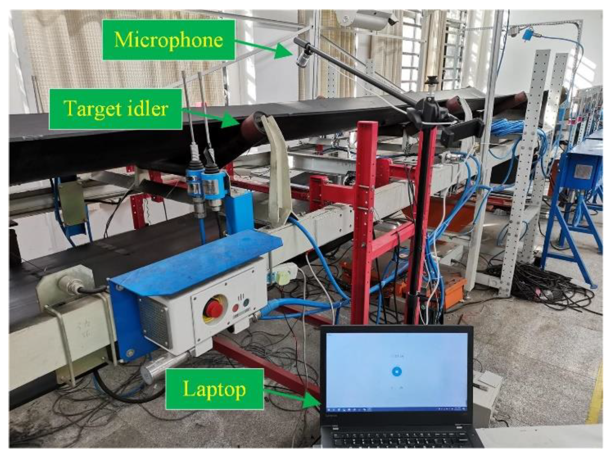
To evaluate the performance of the proposed method, an experimental platform for the fault diagnosis of a belt conveyor idler is built, which is configured to simulate the real working conditions, as shown in Figure 6. The belt conveyor is 7.7 m long and 1.0 m wide, including 5 trough idler sets with a trough angle of 30° and a set spacing of 1.5 m. The target idler is the outer wing idler of the second set, and its parameters are shown in

Table 1. Idler parameters.

Parameter	Value
Length (mm)	375
Diameter (mm)	89
Bearing type	6204
Number of rolling elements	8
Contact angle (°)	10

. The main noise sources are the belt conveyor frame, adjacent idlers, conveyor belt, anti-slanting rollers, motor, etc.

3.2. Data Acquisition

Seventeen faulty idlers are prepared to simulate the typical faults in real conditions and one intact idler is set as a reference, and the fault descriptions are listed in

Table 2. Fault descriptions of idlers/bearings.

Stage	Code	Manifestation	Parameter
Intact	A0	Normal	-
Incipient	A11/A12/A13	Pits on inner ring/outer ring/rolling element	Diameter: 1 mm, depth: 0.5 mm
	A21/A22/A23		Diameter: 2 mm, depth: 0.5 mm
	A31/A32/A33		Diameter: 3 mm, depth: 1.0 mm
Final	B1	Bearing filled with coal particles	Particle diameter < 1 mm
	B2	Rustiness	Level B [31]
	B3	Eccentric rotation	Radial runout tolerance: 2 mm
	C1	Cage damaged	Fracture: 3/8
	C2	Filled with metal debris	Thickness < 0.1 mm
	C3	Raceway wear through	Slot size: 5 × 1 mm
Catastrophic	D1	Jamming	Speed: 0 rpm
	D2	Roller wear through	Speed: 0 rpm, fissure size: 30 × 1.5 cm

. The target idler is replaced with 18 idlers in turn, the load is kept at 50 N, and the belt conveyor is run at the rated speed of 1.6 m/s for 2 h. One hundred samples are taken at equal time intervals at a sampling rate of 44,100 Hz with an omnidirectional microphone about 20 cm away from the target idler and the duration of each sample of 1 s. Finally, 18 × 100 samples are obtained and divided into a training set and a test set with an empirical proportion of 7:3. More details about the data set can be found in our previous work [29].

3.3. Experimental Results and Analysis

Firstly, the number of heads $M$ and iterations $R$ of the DSA block are determined using the control variable method. Secondly, the weighting method is determined by experimental comparison. Thirdly, the performance of the proposed method is compared with that of the existing typical machine-learning and deep-learning methods to demonstrate its superiority, and the negative effects of MFCC and positional encoding on the fault diagnosis model are analyzed experimentally and theoretically.

In order to keep the dimension number of $h_{\mathrm{MF}}$ and $h_{\mathrm{g}}$ roughly equal and the bandwidth of each sub feature moderate, the parameter $n$ (i.e., the number of input sub feature maps of MF-Cov DSA) is set to an empirical value of 31. The proposed idler fault diagnosis model is optimized on the training set by using the stochastic gradient descent with the momentum (SGDM) algorithm. The initial learning rate is 0.001, and it is reduced by half every 2000 cycles. The momentum coefficient, weight decay coefficient, and training epochs are 0.9, 0.0005, and 8000, respectively. The training is performed on the NVIDIA 2080Ti GPU of a desktop.

3.3.1. Super Parameters Determination of the Dynamic Self-Attention Block

The number of heads $M$ and iterations $R$ in the DSA block are the key factors affecting the diagnosis performance. The former determines the diversity of the extracted discriminant features, which is associated with diagnostic accuracy, and the latter affects the inference latency and fitting performance of the model. Since the global DSA module includes an independent DSA block, in order to determine the most appropriate parameters, a fault diagnosis model containing only the global DSA module is used for testing. The input is the A-weighted STFT spectrum of the idler sound sample, with a frame length of 1024, an overlap length of 900 [29], and an FFT length of 1024. When investigating the effect of $M$ or $R$, the other one is fixed as 1 and 2, respectively. The models are configured as different $M$ and $R$ are trained on the training set, then evaluated on the test set, and the results are shown in Figure 7. It can be seen that when $R$ is fixed as 1 and $M$ is 2, the accuracy reaches the maximum value of 93.1%; when $M$ is fixed as 2, $R$ is 1 or 2, the accuracy also reaches the maximum value of 93.1%. However, a larger $R$ means a larger model, which increases the demand for computing power, memory, energy consumption, and inference latency.

As shown in Figure 7a, the accuracy decreases with the increase in $M$, and this is related to the multi-head self-attention mechanism. With the increase in heads, the projection matrices shrink, resulting in a lower dimension of the feature space and loss of useful information. The training losses of all models configured with different $M$ and $R$ converge below 0.001 in the experiment, and with the increase in $R$, as shown in Figure 7b, the accuracy decreases, which reveals that when the number of iterations is larger than 2, the model is overfitted due to the excessive parameters.

Therefore, to ensure optimal idler fault diagnostic accuracy and real-time performance, the number of heads $M$ and iterations $R$ in the DSA block are set to 2 and 1, respectively.

3.3.2. Weighting Method

In order to verify the effect of the weighting method, the proposed models with optimal parameters ($M$= 2, $R$= 1) are trained and tested with A-weighted, C-weighted, and unweighted STFT spectrums of idler sound samples as input, respectively. The accuracy values of fault diagnosis are 94.6%, 94.3%, and 93.5%, respectively, which proves that A-weighted STFT spectrums would improve the accuracy of the fault diagnosis. It is also verified that A-weighting, which enhances the components of the mechanical fault sound, is more conducive to the sound-based idler fault diagnosis than C-weighting, which retains most audible frequency bands.

3.3.3. Performance Comparison and Analysis

The traditional machine-learning algorithms SVM, RF [32], and deep-learning algorithms ResNet-18 [33] and Densenet-121 [34] are selected as the compared algorithms, with the feature extraction algorithms of MFC and STFT, which are both configured with the frame length of 1024, overlap length of 900 [29], and FFT length of 1024. The one-against-one strategy [35] is adopted by SVM to handle the classification of 18 types of faults for its outstanding performance. As for the kernel function, both linear function kernel and radial basis function kernel are evaluated, and the algorithms are abbreviated as SVM-Linear and SVM-RBF, respectively. To facilitate the training and testing, the MFCC feature matrix is flattened into a vector and input into SVM. Since the STFT spectrum is much larger, it is resized using the nearest-neighbor interpolation algorithm, and then flattened into a vector of the same size as the MFCC vector. The number of trees in RF is set to a regular value of 500, and the random feature number of each tree is the square root of the feature vector’s length. MFCC and STFT spectrum matrices are preprocessed in the same way as that of SVM and input to RF. In accordance with the requirements of ResNet-18 and Densenet-121 for input size, the MFCC or STFT spectrum matrix is first resized to 224×224 using the area interpolation algorithm, and then duplicated 3 times along the channel axis and zero-centered as the input. The output dimension of the last fully connected layers in ResNet-18 and Densenet-121 is set to 18 to fit the number of fault types. ResNet-18 and Densenet-121 are initialized with the pre-trained parameters (https://github.com/pytorch/vision/blob/master/torchvision/models/resnet.py, https://github.com/pytorch/vision/blob/main/torchvision/models/densenet.py) and trained in the same way as of the ones in the proposed idler fault diagnosis model. As for the proposed model, when the input is MFCC, which has integrated the information of different frequency bands, the MF-Cov DSA module is not used; when the input is STFT spectrum, it is A-weighted. Each compared algorithm is evaluated on the desktop configured as Intel i7-7820X 3.6 GHz CPU and 16 GB RAM.

Table 3. Performance of each compared algorithm on the test set.

Algorithm	Feature	Accuracy	Latency (ms)	Model Size (MB)
SVM-Linear	MFCC	78.7%	450.0	75.0
SVM-RBF		71.1%	480.0	79.0
RF		64.8%	5.2	2.7
ResNet-18		77.6%	19.2	44.8
Densenet-121		63.9%	53.0	30.4
Ours		90.2%	1.2	0.02
SVM-Linear	STFT spectrum	68.3%	450.9	71.6
SVM-RBF		38.0%	515.6	73.6
RF		68.1%	6.3	2.0
ResNet-18		89.8%	23.0	44.8
Densenet-121		81.9%	54.4	30.4
Ours		94.6%	27.8	3.9

shows the performance of each compared algorithm on the test set. Whether the input is MFCC or STFT spectrum, our model performs best in accuracy with a very lightweight structure: the accuracy is 90.2% and 94.6%, and the inference latency is 1.2 ms and 27.8 ms, respectively. When MFCC is the input, the accuracy of machine-learning algorithms, especially SVM-linear, is better than that of deep-learning algorithms. However, the one-against-one strategy under multi-classes is time-consuming, resulting in poor performance of SVM in latency and model size. When the input is STFT spectrum, deep-learning algorithms, especially ResNet-18, perform better than machine-learning algorithms in accuracy. MFCC is a high-level feature refined on the STFT spectrum and is more suitable for machine-learning algorithms, which reveals that machine-learning algorithms are more dependent on feature saliency and poor in feature extraction. STFT spectrum contains abundant low-level features and is more suitable for deep-learning algorithms that are adept in feature extraction. When dealing with high-dimensional features, the linear function kernel is more conducive to the classification of SVM, since the nonlinear radial basis function kernel further increases the feature dimension and makes SVM overfit.

When the input is MFCC, the diagnostic accuracy of deep-learning algorithms and the proposed model is lower than that when the input is STFT spectrum, indicating that MFCC is not suitable for idler fault diagnosis. Firstly, MFCC maps the broadband power on the natural frequency scale to the Mel frequency scale according to the auditory characteristics of a human ear. Compared with frequency characteristics, MFCC focuses more on speech intelligibility, which is not an effective feature to classify the sound of faulty idlers. Secondly, MFCC retains more low-frequency power, which is mainly generated by the running noise of belt conveyors, and the useful features of medium and high frequency will be weakened or even submerged. Thirdly, MFCC uses DCT transform to extract the envelope of the power spectrum on the Mel frequency scale, and the envelope is mainly used to identify the formant, which is the recognition attribute of speech [36], but there are no formants in the faulty idler sound (as shown in Figure 1).

Based on the prediction results of various faults, as shown in Figure 8, most of the final and catastrophic faults (i.e., B1-B3, C1-C3, D1, D2) can be classified correctly by the proposed model with the input of MFCC and STFT spectrum. When the input is MFCC, small incipient faults (i.e., A12, A13) cannot be classified very well. When the input is STFT spectrum, the accuracy of A12 and A13 increases. With the input of MFCC, SVM-Linear cannot perform well in the classification of idler incipient faults (i.e., A11-A33) despite outperforming the compared machine-learning algorithms. With the input of the STFT spectrum, ResNet-18 misclassifies many of the small incipient faults (i.e., A11, A13).

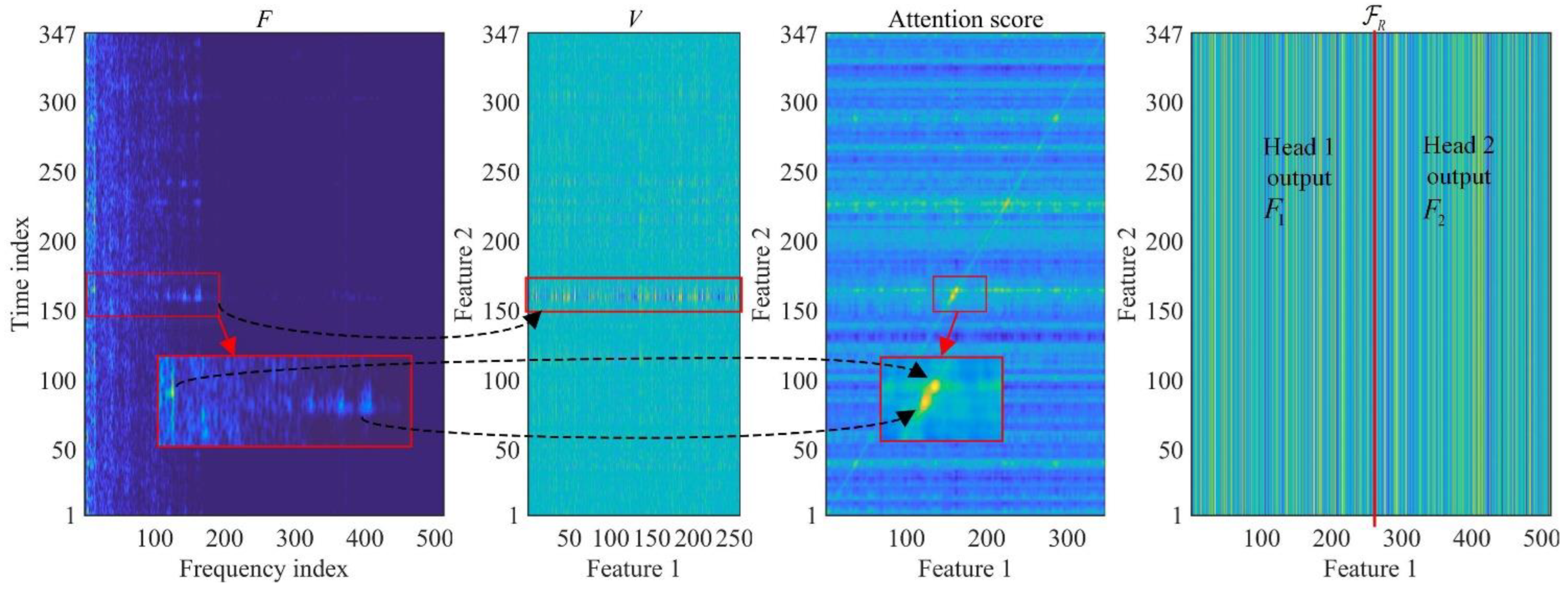
The DSA block is the key point that the proposed model performs better than or equivalent to the compared deep-learning algorithm in accuracy, inference latency, and model size. CNN needs to deepen the network to have a global receptive field, which may lead to the loss of inconspicuous but useful information in the forward transfer of the model, and the network cannot run in parallel in the depth direction. The proposed model can dynamically perceive useful global features via the projection matrices and establish the relationship between elements through the self-attention operation to enhance them, and then discriminant features are obtained via linear projections. With fewer parameters and a shallow network, the model can perceive, enhance, and integrate global features with a lower risk of overfitting and shorter inference latency. Figure 9 visualizes the main working process of DSA in the forward inference process of our model, where the input feature $F$ is STFT spectrum of the idler sound sample with a bearing cage damaged (C1). As the rolling elements collide with each other, intermittent medium- and high-frequency collision sound is emitted, which is shown as the stripes in the red box of the input feature $F$, and this stripe is retained and extended at the corresponding position in $V$. In the figure of attention score (i.e., the result of $softmax \left(Q_{i\_r}^T{K}_{i\_r}/\sqrt{d_K}\right)$), salient spots appear in the corresponding position, which enhances the corresponding features in $V$, while the running noise is not excessively enhanced. In the figure of self-attention output ${ℱ}_R$, elements along the feature 2 axis (corresponding to the time index axis of $F$) differ a little. It can be considered that almost all useful information of $F$ is compressed onto the feature 1 axis, so the extracted feature map is endowed with time translation invariance. Hence, ${ℱ}_R$ is no more suitable for iteration, and this illustrates the rationality of $R$ = 1. The outputs of multi-head self-attention $F_1$ and $F_2$ in ${ℱ}_R$ show different stripes, and this reveals that increasing the number of heads $M$ appropriately will increase the diversity of features.

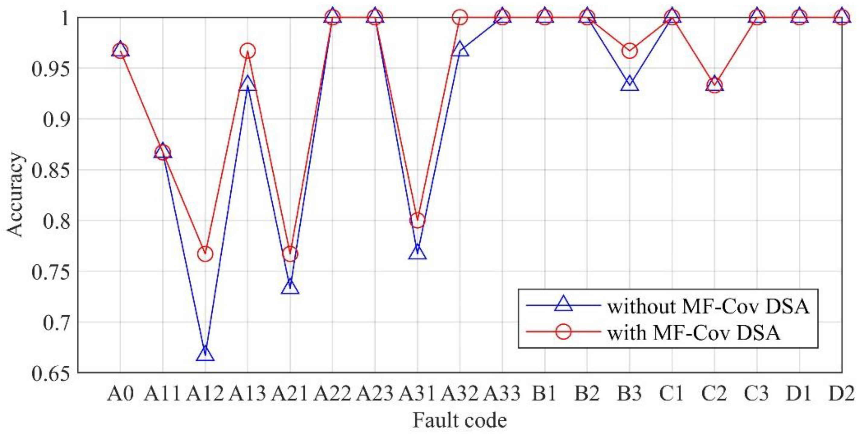
MF-Cov DSA module can significantly improve the diagnostic accuracy of incipient and final faults of idler bearing, especially for small-size idler bearing faults. Figure 10 shows the fault diagnosis results of our model with and without the MF-Cov DSA module. Without it, the diagnostic accuracy of small bearing faults (i.e., inner ring, outer ring and rolling element faults) is at a lower level, especially A12, A21 and A31. With the module, the diagnosis accuracy of almost all fault types has improved. It is worth noting that B3 fault (i.e., eccentric rotation) is characterized by stripes appearing periodically on the STFT spectrum at the same period as the roller rotation. Since the MF-Cov operation extracts the cross-correlation features of modulation information in different frequency bands, the diagnostic accuracy of this fault has also greatly improved.

Positional encoding is not used in the proposed model. Standard Transformer adds positional encoding to the feature map before the input. Typically, it uses the encoding method based on trigonometric functions [22]. Positional encoding is directly added to the input token, which interferes with the weak features of the input, leading to a decline in the accuracy of fault diagnosis. Experiments are carried out to reveal the effects of positional encoding. The STFT spectrums of the samples in the training set and test set are extracted and A-weighted, C-weighted, and unweighted, respectively. Before being used for training and testing, they are positionally encoded. Experimental results show that the diagnosis accuracy is 91.9%, 92.6%, and 93.0%, respectively. Compared with that without positional encoding, the accuracy has declined, especially the A-weighted or C-weighted one. It can be seen from Figure 3 that after they are A-weighted or C-weighted, the low-frequency components are attenuated, especially in the case of A-weighting, the part below 100 Hz is attenuated by more than 10 times. This leads to the following result: after the positional encoding is superimposed, it dominates the attenuated part. Position encoding contains many stripes, which affects the faults characterized by weak stripes, leading to the decline of diagnosis accuracy.

4. Conclusions

In this paper, a fault diagnosis method for belt conveyor idlers based on dynamic self-attention is proposed. Input with the A-weighted time-frequency spectrum of the idler running sound, a shallow network consisting of the MF-Cov DSA module and global DSA module is established to perceive, enhance, and synthesize the multi-frequency and global fault features and predict the fault type. The method improves the detection accuracy of the sound-based fault diagnosis method for incipient faults under complex working conditions, overcomes the dependence of traditional machine learning on feature saliency, and avoids the need to increase the network depth to extract global information in deep learning. The experimental results show that the method can detect and classify idler faults accurately and quickly.

The research provides a novel and practical idea for the fault diagnosis of belt conveyor idlers. The applicability analysis of sound features and the visualized analysis of the fault diagnosis model provides a theoretical and experimental reference for the fault diagnosis of similar equipment. Since the research is mainly aimed at the sound-based fault diagnosis of idlers under the interference of running noise, especially the initial fault of bearings (i.e., the failure of the inner ring, outer ring, and rolling element), it can be applied to the fault diagnosis and health management of related rotating machinery.

References

1. Li, J.; Miao, C.Y. The conveyor belt longitudinal tear on-line detection based on improved SSR algorithm. Optik 2016, 127, 7395–8202. [Google Scholar] [CrossRef]
2. Liu, Y.; Miao, C.Y.; Li, X.G.; Xu, G.W. Research on deviation detection of belt conveyor based on inspection robot and deep learning. Complexity 2021, 2021, 3734560. [Google Scholar] [CrossRef]
3. Vasić, M.; Stojanović, B.; Blagojević, M. Failure analysis of idler roller bearings in belt conveyors. Eng. Fail. Anal. 2020, 117, 104898. [Google Scholar] [CrossRef]
4. Muralidharana, V.; Ravikumarb, S.; Kangasabapathy, H. Condition monitoring of self aligning carrying idler (SAI) in belt-conveyor system using statistical features and decision tree algorithm. Measurement 2014, 58, 274–279. [Google Scholar] [CrossRef]
5. Ravikumar, S.; Kanagasabapathy, H.; Muralidharan, V. Fault diagnosis of self-aligning troughing rollers in belt conveyor system using k-star algorithm. Measurement 2019, 133, 341–349. [Google Scholar] [CrossRef]
6. Peng, C.; Li, Z.P.; Yang, M.J.; Fei, M.R.; Wang, Y.L. An audio-based intelligent fault diagnosis method for belt conveyor rollers in sand carrier. Control Eng. Pract. 2020, 105, 104650. [Google Scholar] [CrossRef]
7. Yang, M.J.; Zhou, W.J.; Song, T.X. Audio-based fault diagnosis for belt conveyor rollers. Neurocomputing 2020, 397, 447–456. [Google Scholar] [CrossRef]
8. Liu, X.W.; Pei, D.L.; Lodewijks, G.; Zhao, Z.Y.; Mei, J. Acoustic signal based fault detection on belt conveyor idlers using machine learning. Adv. Powder Technol. 2020, 31, 2689–2698. [Google Scholar] [CrossRef]
9. Qu, D.R.; Qiao, T.Z.; Pang, Y.S.; Yang, Y.; Zhang, H.T. Research on ADCN method for damage detection of mining conveyor belt. IEEE Sens. J. 2021, 21, 8662–8669. [Google Scholar] [CrossRef]
10. Mao, Q.H.; Ma, H.W.; Zhang, X.H.; Zhang, G.M. An improved skewness decision tree SVM algorithm for the classification of steel cord conveyor belt defects. Appl. Sci. 2018, 8, 2574. [Google Scholar] [CrossRef] [Green Version]
11. Che, J.; Qiao, T.Z.; Yang, Y.; Zhang, H.T.; Pang, Y.S. Longitudinal tear detection method of conveyor belt based on audio-visual fusion. Measurement 2021, 176, 109152. [Google Scholar] [CrossRef]
12. Liu, Y.; Wang, Y.P.; Zeng, C.; Zhang, W.C.; Li, J.Y. Edge detection for conveyor belt based on the deep convolutional network. In Proceedings of the 2018 Chinese Intelligent Systems Conference; Springer: Singapore, 2018; pp. 275–283. [Google Scholar]
13. Gao, Y.; Qiao, T.Z.; Zhang, H.T.; Yang, Y.; Pang, Y.S.; Wei, H.Y. A contactless measuring speed system of belt conveyor based on machine vision and machine learning. Measurement 2019, 139, 127–133. [Google Scholar] [CrossRef]
14. Yasutomi, A.Y.; Enoki, H. Localization of inspection device along belt conveyors with multiple branches using deep neural networks. IEEE Robot. Autom. Lett. 2022, 5, 2921–2928. [Google Scholar] [CrossRef]
15. Jiao, J.Y.; Zhao, M.; Lin, J.; Liang, K.X. A comprehensive review on convolutional neural network in machine fault diagnosis. Neurocomputing 2020, 417, 36–63. [Google Scholar] [CrossRef]
16. Peng, Y.W.; Ma, X.H. A fault diagnosis method of rolling bearings based on parameter optimization and adaptive generalized S-Transform. Machines 2022, 10, 207. [Google Scholar] [CrossRef]
17. Zhang, X.Y.; Qiu, D.Y.; Chen, F.A. Support vector machine with parameter optimization by a novel hybrid method and its application to fault diagnosis. Neurocomputing 2015, 149, 641–651. [Google Scholar] [CrossRef]
18. Jiang, G.Q.; He, H.B.; Yan, J.; Xie, P. Multiscale convolutional neural networks for fault diagnosis of wind turbine gearbox. IEEE Trans. Ind. Electron. 2019, 66, 3196–3207. [Google Scholar] [CrossRef]
19. Li, X.; Zhang, W.; Ding, Q.; Li, X. Diagnosing rotating machines with weakly supervised data using deep transfer learning. IEEE Trans. Industr. Inform. 2020, 16, 1688–1697. [Google Scholar] [CrossRef]
20. Xing, S.; Lei, Y.; Wang, S.; Jia, F. Distribution-invariant deep belief network for intelligent fault diagnosis of machines under new working conditions. IEEE Trans. Ind. Electron. 2021, 68, 2617–2625. [Google Scholar] [CrossRef]
21. Moshrefzadeh, A. Condition monitoring and intelligent diagnosis of rolling element bearings under constant/variable load and speed conditions. Mech. Syst. Signal Pr. 2021, 149, 107153. [Google Scholar] [CrossRef]
22. Vaswani, A.; Shazeer, N.; Parmar, N.; Uszkoreit, J.; Jones, L.; Gomez, A.N.; Kaiser, L.; Polosukhin, I. Attention is all you need. arXiv 2017, arXiv:1706.03762. [Google Scholar]
23. Carion, N.; Massa, F.; Synnaeve, G.; Usunier, N.; Kirillov, A.; Zagoruyko, S. End-to-end object detection with transformers. arXiv 2020, arXiv:2005.12872. [Google Scholar]
24. Chen, H.T.; Wang, Y.H.; Guo, T.Y.; Xu, C.; Deng, Y.; Liu, Z.; Ma, S.; Xu, C.; Xu, C.; Gao, W. Pre-trained image processing transformer. arXiv 2020, arXiv:2012.00364. [Google Scholar]
25. Wu, H.P.; Xiao, B.; Codella, N.; Liu, M.; Dai, X.; Yuan, L.; Zhang, L. CvT: Introducing convolutions to vision transformers. arXiv 2021, arXiv:2103.15808. [Google Scholar]
26. Yang, Z.K.; Garcia, N.; Chu, C.H.; Otani, M.; Nakashima, Y.; Takemura, H. A comparative study of language transformers for video question answering. Neurocomputing 2021, 445, 121–133. [Google Scholar] [CrossRef]
27. Cheon, M.; Yoon, S.J.; Kang, B.; Lee, J. Perceptual image quality assessment with transformers. arXiv 2021, arXiv:2104.14730. [Google Scholar]
28. Krizhevsky, A.; Sutskever, I.; Hinton, G.E. ImageNet classification with deep convolutional neural networks. Commun. ACM 2017, 60, 84–90. [Google Scholar] [CrossRef]
29. Liu, Y.; Miao, C.Y.; Li, X.G.; Ji, J.H.; Meng, D.J. Research on the fault analysis method of belt conveyor idlers based on sound and thermal infrared image features. Measurement 2021, 186, 110177. [Google Scholar] [CrossRef]
30. JJG-2002; Metrological Verification Regulation of P.R. China, Verification Regulation of Sound Level Meters. China Institute of Metrology: Beijing, China, 2002.
31. GB 8923-88; National Standards of P.R. China, Rust Grades and Preparation Grades of Steel Surfaces before Application of Paints and Related Products. National Bureau of Standards: Beijing, China, 1989.
32. Breiman, L. Random Forests. Mach. Learn. 2001, 45, 5–32. [Google Scholar] [CrossRef]
33. He, K.M.; Zhang, X.Y.; Ren, S.Q.; Sun, J. Deep residual learning for image recognition. In Proceedings of the 2016 IEEE Conference on Computer Vision and Pattern Recognition (CVPR), Las Vegas, NV, USA, 27–30 June 2016; pp. 770–778. [Google Scholar] [CrossRef]
34. Huang, G.; Liu, Z.; Maaten, L.; Weinberger, K.Q. Densely connected convolutional networks. arXiv 2016, arXiv:1608.06993. [Google Scholar]
35. Hsu, C.W.; Lin, C.J. A comparison of methods for multiclass support vector machines. IEEE Trans. Neural Netw. 2002, 13, 415–425. [Google Scholar] [CrossRef] [PubMed]
36. Lee, M.; Santen, J.; Mobius, B.; Olive, J. Formant tracking using context-dependent phonemic information. IEEE Trans. Speech Audio Process. 2005, 13, 741–750. [Google Scholar] [CrossRef]
Figure 1. The time domain, frequency domain, and TFD features of the running sound of idlers in different states. (a) Intact state; (b) Bearing outer ring fault; (c) Idler jamming.
Machines 11 00216 g001aMachines 11 00216 g001b
Figure 2. The dynamic self-attention-based idler fault diagnosis method.
Machines 11 00216 g002
Figure 3. Gain curves of A-weighting and C-weighting.
Machines 11 00216 g003
Figure 4. Idler fault diagnosis model based on dynamic self-attention.
Machines 11 00216 g004
Figure 5. The structure of the dynamic self-attention.
Machines 11 00216 g005
Figure 6. Experimental platform for the fault diagnosis of a belt conveyor idler.
Machines 11 00216 g006
Figure 7. The effect of super parameters on the diagnostic accuracy and model size. (a) Number of heads. (b) Number of iterations. In (a) R is fixed as 1, and in (b) M is fixed as 2.
Machines 11 00216 g007
Figure 8. Prediction confusion matrices of the representative algorithms with different input features, (a) Ours-MFCC; (b) Ours-STFT; (c) SVM-Linear-MFCC; (d) ResNet-18-STFT. The color of each grid changes from white to black, corresponding to 0-30. The darker the color is, the more samples of that type of fault are predicted.
Machines 11 00216 g008
Figure 9. Visualized forward inference process.
Machines 11 00216 g009
Figure 10. The diagnostic accuracy of the proposed model for each fault with and without MF-Cov DSA module.
Machines 11 00216 g010