Fault Detection in Aircraft Flight Control Actuators Using Support Vector Machines

Abstract

Future generations of flight control systems, such as those for unmanned autonomous vehicles (UAVs), are likely to be more adaptive and intelligent to cope with the extra safety and reliability requirements due to pilotless operations. An efficient fault detection and isolation (FDI) system is paramount and should be capable of monitoring the health status of an aircraft. Historically, hardware redundancy techniques have been used to detect faults. However, duplicating the actuators in an UAV is not ideal due to the high cost and large mass of additional components. Fortunately, aircraft actuator faults can also be detected using analytical redundancy techniques. In this study, a data-driven algorithm using Support Vector Machine (SVM) is designed. The aircraft actuator fault investigated is the loss-of-effectiveness (LOE) fault. The aim of the fault detection algorithm is to classify the feature vector data into a nominal or faulty class based on the health of the actuator. The results show that the SVM algorithm detects the LOE fault almost instantly, with an average accuracy of 99%.

1. Introduction

Flight reliability is paramount in aerial vehicle platforms, and the classic way to improve flight reliability is through hardware redundancy techniques. However, duplicating actuators in a system to achieve increased flight (control) fault tolerance poses substantial challenge due to their large size and mass and high price. An alternative way to address (and aim to improve) reliability is via analytical redundancy techniques. These techniques can be used to create a health monitoring (HM) system for the aircraft. HM systems can be used to predict failures of a flight control system on an aircraft by detecting faults, with the two main methods for fault detection being data-driven and model-based methods. This paper focuses on the use of data-driven methods to develop a fault detection algorithm for detecting primary flight control actuator faults. Data-driven methods are selected over model-based approaches as the latter normally requires a reasonably accurate mathematical model of a system with a failure, which may not be available. Data-driven methods require no detailed knowledge about the internal dynamics of a system.

The importance of flight reliability in aviation is highlighted by historic events. On 17 September 1908, the world’s first aviation fatality occurred when Orville Wright of the Wright Brothers crashed his aircraft, killing his passenger Thomas Selfridge, during a demonstration flight for the US army [1]. Since this first fatality, there have been monumental improvements in aircraft safety and certification, which now make air travel the safest mode of transport [2]. The main reason for these improvements in safety is due to the continuous evolution of modern aircraft technologies, such as the introduction of fly-by-wire (FBW) flight control systems. This arrangement replaces mechanical linkage and means that pilot inputs do not directly move the flight control surfaces. Instead, the inputs are read by a computer that, in turn, determines how to move the control surfaces to best achieve what the pilot wants, in accordance with which of the available flight control laws is active [3]. In 1984, the Airbus A320 became the first airliner to fly with an all-digital FBW control system [4]. FBW provides increased safety and efficiency, reduces workload for pilots, and enhances weight reduction and flight envelope protection.

Currently, a manned aircraft has stringent reliability requirements, which allow for less than a single catastrophic malfunction per ${10}^9$ h of operations. For decades, aircraft manufacturers have achieved this level of reliability via the use of hardware redundancy (HR) throughout the flight control system design, encompassing multiple control surfaces, actuation systems, sensors, and flight computers. Future generations of flight control systems, such as those for UAVs, are likely to be more adaptive and intelligent to cope with the additional safety and reliability requirements due to not having a pilot on board. Improving flight reliability of UAVs is considered to be one of the main concerns in integrating these aircraft into civil airspace [5]. According to a study conducted by the US Office of the Secretary of Defense, about 80% of flight incidents with UAVs are due to faults affecting sensors or flight control surfaces [5]. This need to improve reliability necessitates the development of sophisticated techniques that deviate from traditional methods. These techniques will need to provide fault diagnosis and fault tolerance in a timely and accurate manner. To allow autonomous aerial vehicles to continue their missions, there is an absolute necessity to identify unexpected changes (faults) in the system before they lead to a complete breakdown (failure) [6].

Redundancy is the main method of improving flight reliability and detecting faults. As mentioned, hardware redundancy techniques have been in use for decades. Traditionally, voting algorithms are used to check for consistency of behaviour among HR flight control subsystems and usually provide direct fault detection and identification. HR, however, carries a cost, payload, and power consumption penalty. This method leads to additional costs and increased weight, which are an impediment to autonomy. One of the main selling points of UAVs is the cost reduction benefit, which could be up to 40% for regional air mobility [7]. There is another type of redundancy called analytical redundancy that improves flight reliability and can detect faults. Analytical redundancy (AR) is the use of mathematical relations between real-time measured and estimated variables to detect and predict possible faults. Analytical redundancy incurs less weight and cost when compared to HR. The need for a faster, cleaner, and more energy-efficient aircraft has also made the use of analytical redundancy methods essential as the number of redundant components is reduced, and thus the aircraft mass is reduced, which increases the efficiency of an aircraft. The research work in this paper focuses on the use of analytical redundancy techniques.

Through the use of AR or HR techniques, faults on an aircraft can be detected. As defined in [8], a fault is an unpermitted deviation of at least one characteristic property or parameter of the system from acceptable/usual/standard conditions. Fault detection is the determination of the presence of faults in a system and of their times of occurrence. Fault detection is important for flight safety [9,10,11]. It is generally followed by fault isolation to determine the type and location of the faults. This complete process is called fault detection and identification (FDI). An efficient FDI system should be capable of monitoring the health status of actuators [12]. The three types of faults pertinent to aircraft are sensor faults, actuator faults, and process faults. This study will focus on the fault detection of an aircraft’s primary flight control actuators. Specifically, this research will focus on the loss-of-effectiveness (LOE) fault.

Fault detection via analytical methods can be categorised into two methods: model-based and data-driven methods. A model-based method is when the detection and isolation of faults in a system come from a comparison of the system’s available measurements with a priori information represented by the system’s dynamic model. In model-based approaches, Kalman filters are quite popular [13]. Although such model-based techniques have their advantages in terms of on-board and real-time implementation capabilities, their reliability for health monitoring often decreases as the system nonlinearities, complexity, and modelling uncertainties increase [14]. Data-driven approaches use information from previously collected data to identify the characteristics of faults. This information is then used to predict the future trend without any particular physical model of the system [15]. The database consists of observations of the monitored values, such as the state variables. The diagnosis can essentially be viewed as pattern recognition where new measurements are classified in predetermined models [5]. The two main differences between model-based approaches and data-driven approaches are the availability of a physical model and the use of training data to identify the characteristics of a damage state [15]. For this research the following two data-driven methods will be investigated: Support Vector Machines (SVMs) and Neural Networks (NN).

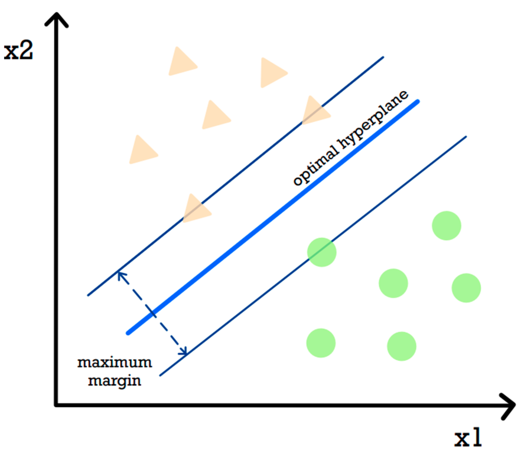
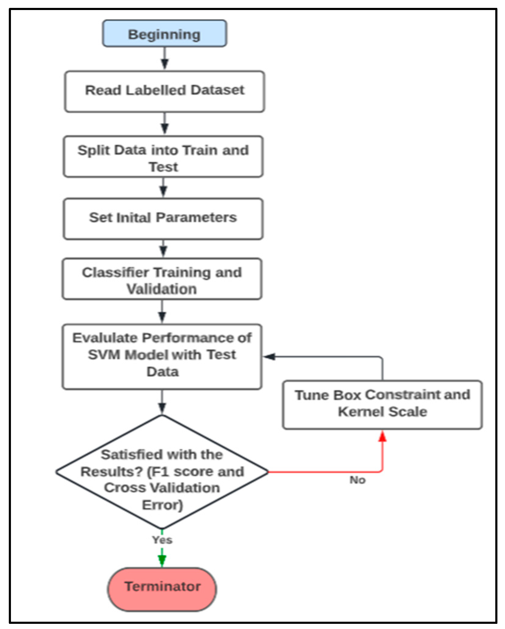
Support Vector Machine (SVM) is a supervised machine-learning classification algorithm. There are two main phases of training and prediction. Supervised learning requires labelling the fault cases in the training data. In the training phase, the model learns to fit the labelled data that are inputted into the SVM algorithm. The labelled dataset is first divided into two, where 80% of the data are for training and 20% of the data are for testing. The objective of SVMs is to find an optimal hyperplane with the maximum possible margin support vectors in a given data set. SVMs avoid local minima, to which Neural Networks are inherently prone. If the data are not linearly separable by the hyperplane, a kernel trick is used to transform the input space to a higher dimensional space. In [16], a SVM model is used to classify flight control actuator faults. The output of a SVM model is either nominal or faulty. Most machine-learning and deep-learning algorithms have parameters that can be adjusted that are called hyperparameters. Hyperparameters are important in building robust and accurate models. Hyperparameters can be tuned using Bayesian optimisation techniques to prevent the model from overfitting or underfitting. The results obtained in [16], using simulated data from a non-linear aircraft model to investigate a loss of actuator effectiveness, were promising with a classification accuracy of ${10}^{-5}$.

Neural Networks (NN) are considered the main class of traditional non-parametric detection methods. A NN algorithm is a representative data-driven method in which a network model learns a way to produce a desired output, such as the level of degradation, by reacting to the given inputs, such as time and usage conditions. The neurons in the network are nonlinear information-processing elements, and the interconnections between these neurons are known as weights. These weights are learned through supervised training algorithms, where the training data contain the inputs and their corresponding output labels. Using a NN for fault detection is a difficult practice, which involves the selection of the structure of the network, the number of neurons, the activation function, and the learning rate. There is no universal procedure to establish a proper NN, and there is no best structure for aircraft fault diagnosis [17]. For data-driven fault detection in an aircraft, NNs have mainly been used for fault detection of aircraft engines and air sensors, rather than actuation systems [14,18,19]. In [20], the application of NNs for the fault diagnosis of rotor failure in a hexacopter is examined. To monitor the rotor faults in real time, a time-series-assisted neural network was used, which showed promising results as the classification accuracy was 98.8%. With regard to testing NNs with real aircraft data, there have been few attempts as the uncertainty in the data caused by bias and noise impacts the weight parameters. This issue has been noted, with current research being shifted towards adaptive neural networks. In [21], the researchers demonstrated that by updating the NN weights with extended Kalman filter algorithms, the accuracy and response time of a NN-based fault detection system for aircraft actuator failures improved. However, the downside of this approach is that a high-fidelity model of the aircraft is required as well as a data-driven neural network.

Given the above overview of the two methods, SVM is the chosen approach in this work. The rationale is that a SVM method avoids the local minima to which NNs are inherently prone, and there is also a more structured method to tune the hyperparameters of a SVM method.

The work in this paper strongly contributes to enabling flight reliability by proposing a SVM data-driven fault diagnosis method to detect and identify faults in an aircraft flight control actuation system. The nonlinear model of the motion of a UAV is used to develop and validate the approach. The performance of the SVM FDI algorithm is tested and validated for failures (loss of effectiveness) of elevator and aileron actuators. The proposed algorithm demonstrates fast detection and isolation time and high accuracy despite the noisy data.

This paper is structured as follows. First, the nonlinear model of the aircraft, together with the longitudinal flight controller, is presented in Section 2. Secondly, the design and implementation of the SVM fault detection method is provided in Section 3. Lastly, the method is validated and analysed in Section 4, while Section 5 presents a discussion of the results and concludes the paper.

2. Modelling of the Nonlinear Aircraft Model and Longitudinal Flight Controller

The primary objective of this project is to develop a mathematical model of a vertical take-off and landing (VTOL) aircraft with failure modes. A longitudinal flight controller is also designed so that closed-loop fault diagnosis can be performed. The aircraft model is not used as part of the fault detection algorithm. The purpose of the model is to provide a platform to simulate flight data and faults. The aircraft chosen is a SWIFT VTOL aircraft, and the aircraft is modelled in Simulink and MATLAB using the equations of motion. The aircraft was originally designed by MFE Fighter VTOL and has been modified and manufactured by TETRA DRONES. The SWIFT VTOL was designed for research purposes at Cranfield University. It is a fixed-wing aircraft with a wingspan of 2.4 m. The aircraft can take off and land vertically as there are four rotors attached to the aircraft in a quadcopter-type setup; this can be seen in Figure 1.

Table 1. Details of SWIFT geometry.

Vertical Fin (NACA 0010)		Tail Wing (NACA 0010)
Semi Span	$0.34 \mathrm{m}$	Semi Span	0.38 m
MAC	$0.21 \mathrm{m}$	MAC	0.20 m
Main Wing (NACA 6412)		Entire Aircraft
Semi Span	$1.21 \mathrm{m}$	Length	1.44 m
MAC	$0.31 \mathrm{m}$	Mass	10 kg
Surface Area	$0.36{ \mathrm{m}}^2$	Cruise Speed	15 m/s
		${\mathit{I}}_{\mathit{x}\mathit{x}}$	1.25 kg/m3
		${\mathit{I}}_{\mathit{y}\mathit{y}}$	1.01 kg/m3
		${\mathit{I}}_{\mathit{z}\mathit{z}}$	2.24 kg/m3
		${\mathit{I}}_{\mathit{x}\mathit{z}}$	0.084 kg/m3

below presents the important details of the SWIFT geometry.

2.1. Equations of Motion for the Nonlinear Aircraft Model

The equations of motion used in the modelling of the SWIFT aircraft are presented here. First, the kinematic equations are presented, followed by the dynamic equations. The position of the aircraft in a fixed-earth axis is given by ${\mathit{x}}_e={\left[x_e, y_e, z_e\right]}^T$, and for the body axis, it is given by ${\mathit{x}}_b={\left[x_b, y_b,z_b\right]}^T$. The velocities are obtained by the derivation of the positions. The fixed earth velocities are given by ${\mathit{v}}_e={\left[v_e{}_x,v_e{}_y,v_e{}_z\right]}^T$, and the body axis velocities are given by ${\mathit{v}}_b={\left[v_b{}_x, v_b{}_y,v_b{}_z\right]}^T$. The change of coordinates from the fixed earth axis to the body axis is governed by the Euler angles ${\left[\phi ,\vartheta ,\psi \right]}^T$ for roll, pitch, and yaw. To obtain the velocity of the aircraft relative to the fixed-earth axis, the following kinematic transformation is performed:

$$\left[\begin{array}{c}{v}_e{}_x\\ v_e{}_y\\ v_e{}_z\end{array}\right]=\left[\begin{array}{ccc}cos \psi cos\theta & -sin\psi cos\varphi +cos\psi sin\theta sin\varphi & sin\psi sin\varphi +cos\psi sin\theta cos\varphi \\ sin\psi cos\theta & cos\psi cos\varphi +sin\psi sin\theta sin\varphi & -cos\psi sin\varphi +sin\psi sin\theta cos\varphi \\ -sin\theta & cos\theta sin\varphi & cos \theta \cos \varphi \end{array}\right]\left[\begin{array}{c}u\\ v\\ w\end{array}\right]$$

(1)

The angular rates in the body axis, ${\omega }_b={\left[p,q,r\right]}^T$, are also translated to the fixed-earth axis and are expressed from the derivatives of the Euler angles. The Euler rates are obtained from the inversion of this matrix, which gives Equation (2). Equations (1) and (2) represent the kinematic equations of the aircraft.

$$\left[\begin{array}{c}\dot{\varphi }\\ \dot{\theta }\\ \dot{\psi }\end{array}\right]=\left[\begin{array}{ccc}1& sin\varphi tan\theta & cos\varphi tan\theta \\ 0& cos\varphi & -rsin\varphi \\ 0& sin\varphi sec\theta & cos\varphi sec\theta \end{array}\right]\left[\begin{array}{c}p\\ q\\ r\end{array}\right]$$

(2)

Force and momentum equations are required to complete the mathematical model of the aircraft. This section starts by outlining each of the forces acting on the SWIFT aircraft and then moves on to outline the moments. The sum of the external forces in the body-fixed coordinate frame is equal to the rate of change of linear momentum of the system. In the body frame, the force equation takes the following form:

$$\left[\begin{array}{c}{\dot{v}}_b{}_x\\ {\dot{v}}_b{}_y\\ {\dot{v}}_b{}_z\end{array}\right]=\frac{1}{m}\left(F_{Total}\right)-\left[\begin{array}{c}p\\ q\\ r\end{array}\right]\times \left[\begin{array}{c}{v}_b{}_x\\ v_b{}_y\\ v_b{}_z\end{array}\right]$$

(3)

The total forces consist of gravity forces, aerodynamic forces, control surface forces, quadrotor forces, and thrust forces. The total force acting on the model is presented in the following equation:

$$F_{Total }=F_g+F_{aero}+F_{control}+F_{thrust}$$

(4)

Firstly, the gravitational force acting along the body axis is determined. The gravity force is a body force and acts in the $z_{Earth}$ axis direction. The components of this force in the perturbed $x$, $y,$ and $z$ directions are given by the following equations:

$$F_g{}_x=-mg\mathit{sin}\theta$$

(5)

$$F_g{}_y=mg\mathit{sin}\phi \mathit{cos}\theta$$

(6)

$$F_g{}_z=mg\mathit{cos}\phi \mathit{cos}\theta$$

(7)

Whenever the aircraft is disturbed from its equilibrium, the aerodynamic balance of the aircraft changes. The process of obtaining aerodynamic forces provides a considerable challenge due to the subtle interactions present in the motion. The equation for aerodynamic forces is given as follows:

$$F_{aero}=\overline{q}{s}_{ref}\left[\begin{array}{c}{C}_x\left(\alpha ,\beta ,V\right)\\ C_y\left(\alpha ,\beta ,V\right)\\ C_z\left(\alpha ,\beta ,V\right)\end{array}\right]$$

(8)

where $\overline{q}$ is the dynamic pressure; $s_{ref}$ is the aircraft reference area; $\alpha$ is the angle of attack; $\beta$ is the sideslip angle; and $V$ is the true airspeed. The aerodynamic coefficients, $C_{x,y,z}$, are non-linear functions. The values for the aerodynamic coefficients are calculated using DATCOM, which is a computer program that calculates non-dimensional aerodynamic coefficients and derivatives.

When control surfaces (such as the elevator or the aileron) are deflected, an additional force is created, i.e., $F_{control}$. The aerodynamic coefficients for the elevator and the aileron are obtained using DATCOM. The value of the control surface force is obtained from a function of the control input, the Mach number, the altitude, and the angles of attack and sideslip. The quadrotor force, $F_{quad}$, is used to represent the additional force needed during take-off and landing. This force acts in the z-axis and can be found by using a 1-D lookup table, which finds the thrust value in Newtons equivalent to the RPM of each of the four motors. The last force is the thrust force, $F_{thrust}$. An assumption is made that the thrust is aligned with the centre of gravity, and the motors and motor supporting rods do not produce extra drag during a longitudinal flight. The thrust force in forward flight in Newtons is calculated by using a 1-D lookup table, where a curve relating the thrust in a percentage to an overall RPM is calculated.

The external forces that act on the aircraft create moments. The moment equation is given with the following equation:

$$\dot{\omega }=I^{-1}\left(-\omega \times I\omega +M_{total}\right),$$

(9)

where $\omega ={\left(p, q,r\right)}^T$ and I is the inertia matrix. The following equation represents the sum of the total moments acting on the aircraft:

$$M_{total}=M_{aer{o}_{total}}+M_{cs}+M_{thrust}$$

(10)

The aerodynamic moments, $M_{aero}{}_{total}$, that act in the body axis are given by the following equation:

$$M_{aer{o}_{total}}=\left[\begin{array}{c}{L}_{aero}\\ M_{aero}\\ N_{aero}\end{array}\right]=\overline{q}{s}_{ref}\left[\begin{array}{c}b C_l\left(\alpha ,\beta ,V,\omega \right)\\ \overline{c} C_m\left(\alpha ,\beta ,V,\omega \right)\\ b C_n\left(\alpha ,\beta ,V,\omega \right)\end{array}\right]$$

(11)

where $C_l$, $C_m, \mathrm{and} C_n$ are the roll, pitch, and yawing moment coefficients, and $b \mathrm{and} \overline{c}$ are the semispan and the mean aerodynamic chord. Equation (11) is similar to Equation (8) obtained for the aerodynamic forces. The aerodynamic coefficients for $M_{aero}{}_{total}$ are obtained by using DATCOM. $M_{cs}$ represents the additional moments created when the control surfaces are deflected. Using the aerodynamic coefficients obtained from DATCOM, the moments due to the deflection of the elevator and aileron control surfaces can be ascertained. The values of the control surface moments are obtained from a function of the control input, the Mach number, the altitude, and the angles of attack and sideslip. Next, the moment produced due to thrust is $M_{thrust}$. An assumption is made that the thrust is aligned with the centre of gravity, and, therefore, $M_{thrust}$ is equal to zero. For simplification purposes, the propellor torque reaction from the four motors, which are used for a vertical take-off and landing, is not considered.

2.2. Longitudinal Flight Controller

Fault detection and isolation (FDI) methods are normally applied to open-loop systems. However, a FDI system might have significant interaction with the control system. To study the effect of a control system on FDI, as well as to obtain a better overall system performance and a lower overall complexity, the control system and fault detection system are simultaneously designed in this study.

For the SWIFT VTOL model, a linear–quadratic regulator (LQR) flight controller is proposed. An overview of the LQR design (schematic) is shown in Figure 2. The LQR method provides the “best” (or optimal, subjected to the weighting matrices’ choice for the states and the control effort) gain matrix $K$, without explicitly choosing to place the closed-loop poles in particular locations. Once the longitudinal state-space (SS) model of the SWIFT aircraft is generated, the SS model related to the elevator input is determined. The feedback states are the chosen longitudinal states: $x_{lon}=[u w q$ $\theta$]. The LQR method involves solving a cost function, which takes the following form:

$$J={{\displaystyle \int }}_0^{\infty }(x^{T}Qx+u^{T}Ru) dt$$

(12)

The goal is to develop a control strategy, $u=-Ku$, to minimise Equation (12). The variable $x$, contains the feedback states, which in this problem is $x_{lon}$. The matrices $Q$ and $R$ weight the cost of deviations of the state from a steady state and the cost of actuation. These matrices are often diagonal, and the diagonal elements are tuned to change the relative importance of the control objectives. Because of the well-defined quadratic cost function in Equation (12), the optimal controller gain $K$ can be solved. This type of control technique optimally balances the system error and the control effort based on the cost.

2.3. Fault Scenarios and Tests

Several tests are performed using the SWIFT model in order to generate simulated flight data for the SVM model. Figure 3 illustrates the actuator and control block from the SWIFT Simulink model. The elevator and aileron control signals include a timed switch, which applies a gain to the signal after a set time, allowing the loss-of-effectiveness (LOE) fault to be simulated. Looking at the elevator blocks, a gain of 0.5 is applied to the signal to reflect a LOE fault of 50% after the nominal time. Various levels of LOE actuator faults are modelled by modifying the gain blocks in the Simulink model.

Overall, by changing other parameters in the SWIFT VTOL model (such adding noise and closing the loop), the following tests are performed:

• Elevator actuator with a LOE fault.
• Aileron actuator with a LOE fault.
• Cross-correlation test between the elevator and aileron faut detection models.
• Elevator actuator LOE fault with noisy measurements.
• Elevator actuator LOE fault in a closed loop.

3. Design and Implementation of the SVM Fault Detection Method

3.1. Support Vector Machine (SVM) Preliminaries

Support Vector Machine is a relatively new supervised machine-learning approach for classification. In binary classification, the inputs are divided into two classes, and the learner must produce a model that assigns unseen inputs to one of these classes. SVM has the potential of handling large feature spaces. This is because the training of a SVM is carried out so that the dimension of the classified vectors does not have as much of an influence on the performance of the SVM as it would have on the performance of conventional classifier. This description of the model follows that outlined in [22]. The training dataset is $\left(x_i,y_i\right)$ for $i=1,2,\dots ,N$, where $N$ is the number of samples. The dataset has two classes, which is the positive class and the negative class. The positive class obtains the value of $y_i=1,$ and the negative class obtains the value of $y_i=-1$. The linear classifier takes the following form:

$$f\left(x\right)=w^{T}x+b$$

(13)

where $w$ is weight vector and $b$ is the bias. Given this equation, there is a hyperplane $f\left(x\right)=0$ that classifies the given dataset. If the samples associated with the labels can be separated linearly, two hyperplanes can be found that separate the samples, and there will be no points between them. This is visualised in Figure 4 which is inspired by [16].

The region between the two hyperplanes is called the margin. The principal aim of SVM is to maximise this margin, as shown in Figure 4, in order to improve its generalisation ability. This optimisation is given by the following equation:

$$\begin{array}{c}min\Vert w{\Vert }^2\\ \mathrm{subject} \mathrm{to} y_i\left(w^T{x}_i+b\right)\ge 1 for i=1,2,\dots N \end{array}$$

(14)

This is known as the primal problem; it is the constrained optimisation problem. As it is quadratic, there is one single global minimum, which avoids the problem associated with neural networks. Another way to represent SVM mathematically is the dual problem. The dual problem form is beneficial when using SVM to solve nonlinear classification tasks. The classifier takes the form seen in Equation (15), where $a_i$ is the Lagrange multiplier.

$$f\left(x\right)={\displaystyle \sum }_{j=1}^N{a}_i{y}_i\left(x_i^{T}x\right)+b$$

(15)

One way to deal with nonlinearly separable data is to use kernels. Kernels are the core of efficient SVM classifiers and increase computational efficiency. By applying kernel functions, the samples are mapped onto a higher dimensional feature space, in which linear classification is possible. A kernel function is the inner product between samples, where $k\left(x_j,x_i\right)=\mathsf{\Phi }{\left(x_j\right)}^T\mathsf{\Phi }\left({\mathrm{x}}_{\mathrm{I}}\right)$, and $\mathsf{\Phi }\left(x\right)$ is a feature map. The process of calculating the higher-dimensional relationships without transforming the data is called the kernel trick. This trick is important as it reduces the amount of computation required for SVM as the mathematics required to transform the data from low to high dimensions is avoided. By applying the kernel function, Equation (15) becomes Equation (16), as the $x$ vector is mapped to the feature map:

$$f\left(x\right)={{\displaystyle \sum }}_{j=1}^N{a}_i{y}_i\left(\mathsf{\Phi }{\left(x_i\right)}^T\mathsf{\Phi }\left(\mathrm{x}\right)\right)+b$$

(16)

In the dual problem, the SVM algorithm can be formulated to learn a linear classifier by solving an optimisation problem over the parameter $a_i$, the Lagrange multiplier. Instead of minimising over $w$ and $b$, which are subjected to constraints, we can maximise over $a$. This can be expressed as follows:

$$\max L\left(a\right)={{\displaystyle \sum }}_{i=1}^N{a}_i-\frac{1}{2}{{\displaystyle \sum }}_{j,k=1}^N{a}_i{a}_j{y}_i{y}_{j}k\left(x_i,x_j\right)$$

(17)

$$subject to a_i\ge 0 and {\displaystyle \sum }_{i=1}^N{a}_i{y}_i=0$$

(18)

If we then take the derivate w.r.t $a$ and set it equal to zero, we obtain the following solution and can solve for $a_i$:

$$\begin{array}{c}{\displaystyle {\displaystyle \sum }_{i=1}^N}{a}_i{y}_i=0\end{array}$$

(19)

$$\begin{array}{c}0\le a_i\le C \end{array}$$

(20)

where $C$ is the regularisation parameter or the box constraint. When $C$ is small, the constraints are ignored, and there is a large (soft) margin between the classified data sets. When $C$ is large, there is a narrow margin, and when $C=\infty ,$ there is a hard margin. Once $a_i$ is solved, the weights, $w$, for the maximal margin separating the hyperplane is found. Therefore, after training and finding $w$, given an unknown point $u$ measured on features $x_i$, we can classify the point by evaluating the sign of $f\left(x\right)$ as defined by the following equation:

$$\begin{array}{c}f\left(x\right)=sign\left({\displaystyle {\displaystyle \sum }_i^N}{a}_i{y}_{i}k\left(x_i,u\right)+b\right)\end{array}$$

(21)

3.2. SVM Training

The aim of the SVM algorithm is to classify the feature vector data from the SWIFT model into either a nominal or faulty class. The nominal data are the data when the actuator does not have a fault, and the faulty data are the data when the actuator has a fault. The method follows the workflow chart in Figure 5.

3.2.1. Training and Cross-Validating the SVM Model

The MATLAB function fitcsvm uses the training set of the feature vector data to train the model. Within the option for the fitcsvm, the Gaussian kernel function is chosen, and the class names are set as nominal and faulty. The kernel scale and the box constraint are both set to their default value, which is 1. The trained SVM model is then cross-validated through the k-fold method. K-fold cross-validation is the process of creating a model that is cross-validated using a set number of “k-folds”. The function crossval uses a 10-fold cross-validation on the trained model. The function returns a cross-validated machine learning model. The cross-validated model is passed through kfoldLoss, which returns the classification loss obtained by the model. This value of the classification loss is used to investigate the performance of the SVM model. For each of the 10-folds, the function computes the classification loss for the validation-fold observations using a classifier trained on the training-fold observations. Cross-validation is essential as it estimates the out-of-sample misclassification rate. Having a low cross-validation classification loss is essential for a robust model.

3.2.2. Evaluating the Performance of the SVM Model

Once the model is trained and cross-validated, the performance of the model can be evaluated. The performance of the SVM model is evaluated using an F1 score. An F1 score is a measure of a model’s accuracy on a dataset. An F1 score is a way of combining the precision and recall of the model. The highest F1 score is 1, and the lowest F1 score is 0.

Precision is a measure of the result relevancy, and recall is a measure of how many truly relevant results are returned. Precision and recall are derived from the confusion matrix. The confusion matrix takes the form: $CM=\left[\begin{array}{cc}TP& FP\\ FN& TN\end{array}\right]$. This matrix can be calculated in MATLAB by using the function confusionmat. This function compares the predicted labels from the model to the known labels and returns a confusion matrix for the classification problem. The matrix contains the number of true positives, true negatives, false positives, and false negatives. The meaning behind these parameters for this study, unless stated otherwise, is outlined in

Table 2. Description of the parameters in the confusion matrix.

TP—Model correctly identifies nominal data as nominal.

TN—Model correctly identifies faulty data as faulty.

FP—Model classifies a faulty situation as nominal.

FN—Model classifies a nominal situation as faulty.

. The false positive row is highlighted in red, as having a false positive result is the worst error for this case since the fault can go unnoticed and develop into a failure.

Once the precision and recall are calculated, an F1 score is computed by using Equation (22).

$$\begin{array}{c}\mathrm{F}1 \mathrm{Score}=\frac{2\times recision\times recall}{precision+recall }=2\times \frac{\left(\frac{TP}{TP+FP}\right)\times \left(\frac{TP}{TP+FN}\right)}{\left(\frac{TP}{TP+FP}\right)+\left(\frac{TP}{TP+FN}\right)} \end{array}$$

(22)

Another way to evaluate the performance of a fault detection algorithm is to look at the fault detection time. This can be obtained by looking at the posterior probability for the SVM model. The method to obtain the posterior probability is based on [23]. Firstly, the MATLAB function fitSVMPosterior is used. This function takes in the trained SVM model and returns the ScoreSVMModel, which is a trained SVM classifier containing the optimal score-to-posterior-probability transformation function for two-class learning [24]. In order to estimate the posterior probabilities, the ScoreSVMModel and the out-of-sample data are passed through the function predict. The function predict returns the posterior probabilities, which indicate the likelihood that a label comes from a particular class. The posterior probabilities can be plotted against time to obtain an indication of the detection time of the SVM model.

3.2.3. Tuning the SVM Model

If the results are poor, such as a low F1 score or a high cross-validation classification error, the hyperparameters can be tuned. The parameters, including the box constraint, $\mathrm{C}$, and the kernel scale, $\mathsf{\sigma }$, are tuned to avoid overfitting, which is the main issue in parametric discrimination approaches, such as neural networks. The hyperparameters are tuned using the Bayesian optimisation function bayesopt. Optimisation, in its most general form, is the process of locating a point that minimises a real-valued function called the objective function. Bayesian optimisation is the name of one such process. Bayesian optimisation internally maintains a Gaussian process model of the objective function and uses objective function evaluations to train the model. The objective function in this case is the kfoldLoss classification error. During the optimisation, the objective function is printed with respect to the bayesopt function evaluations. The objective is to converge after 30 evaluations for a variety of box constraint and kernel scale values. Once the model has converged, the optimum results for the hyperparameters are fixed in the fitcsvm function. This tuned model can then be re-evaluated using the test data.

4. Analysis and Validation of the Fault Detection Method

4.1. Processing the Dataset

The first step is obtaining the dataset from the SWIFT Simulink model in which a fault has been injected into the actuator model. Different fault situations and tests to evaluate the robustness of the model are performed. These tests are listed above and detailed in this section. The simulation is run for $t_s=180 \mathrm{s}$, and the fault is set to occur at $t_F=120 \mathrm{s}$. The data required for the SVM model are the signal output values of the body acceleration in each axis, $a_x$, $a_y,$ and $a_z$, and the body angular rates, $p$, $q,$ and $r$. This combined dataset is called the feature vector dataset, and these variables are chosen as they give a good dynamic representation of the model. The simulation time array, $t_s$, is also required. The time array is not included in the feature vector as it is only used to assist in labelling the dataset. The time array and the feature vector dataset have the same number of points. By examining $t_s$, the datapoint corresponding to 120 s is found. All the datapoints in the feature vector $<t_F$ are labelled as nominal, and the datapoints $\ge t_F$ are labelled as faulty. After the data are labelled, they are normalised. The data are normalised to make the values of the features change within the same order of magnitude. Next, the labelled dataset is split into two portions, in which 80% of the data are used for training and 20% of the data are used as the test set to evaluate the classifier.

4.2. SVM Model for Elevator Actuator LOE Fault

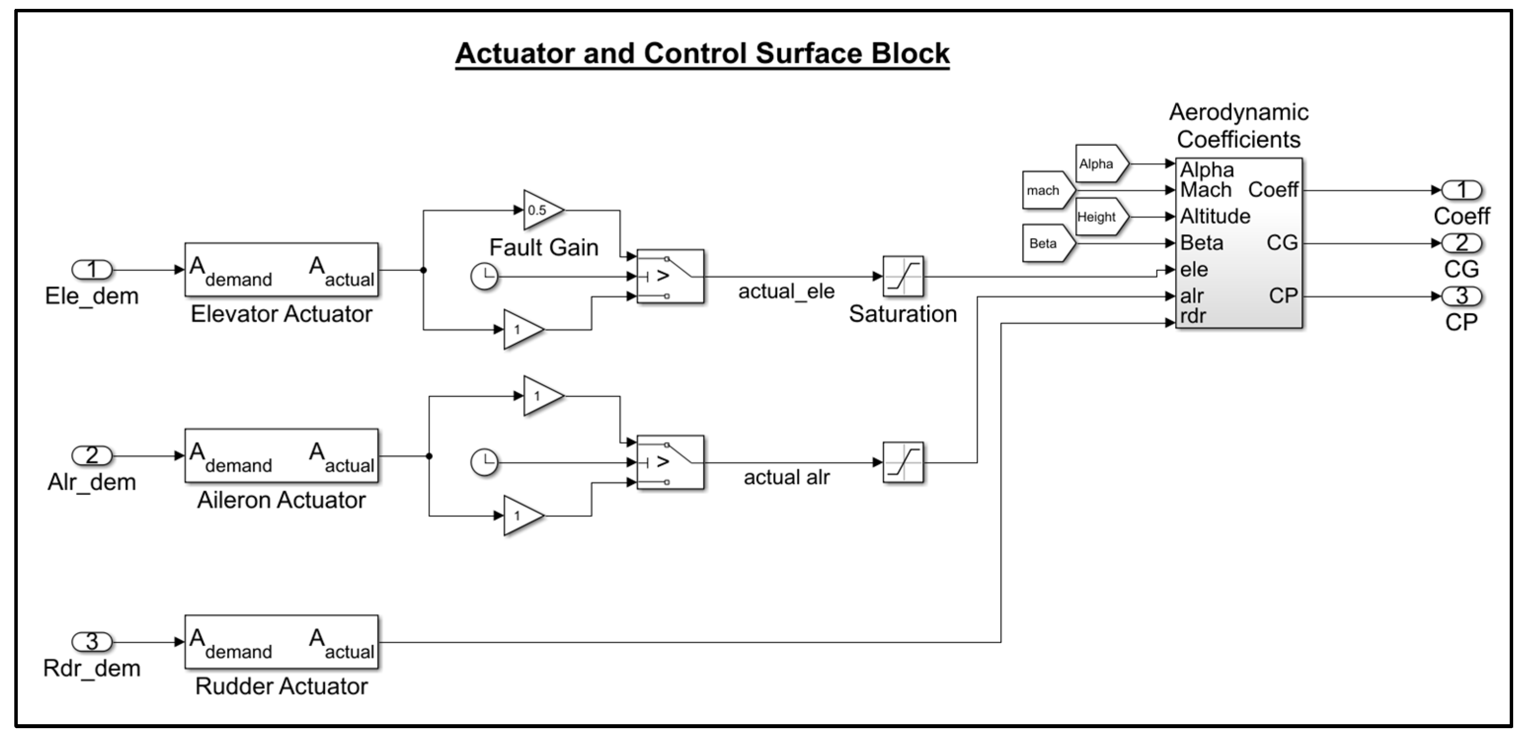
A fault is injected into the elevator actuator by using the signal switch block in Simulink. The signal is switched after 120 s to a gained value of the signal, which is used to simulate the loss-of-effectiveness fault. Three tests are performed, and the following percentages of loss of effectiveness are simulated: 25%, 50%, and 75%. The actual elevator control signal for each percentage can be seen in Figure 6, where after $t=120 \mathrm{s}$, there is a decrease in the actual elevator signal from the trim value of 1.476 degrees.

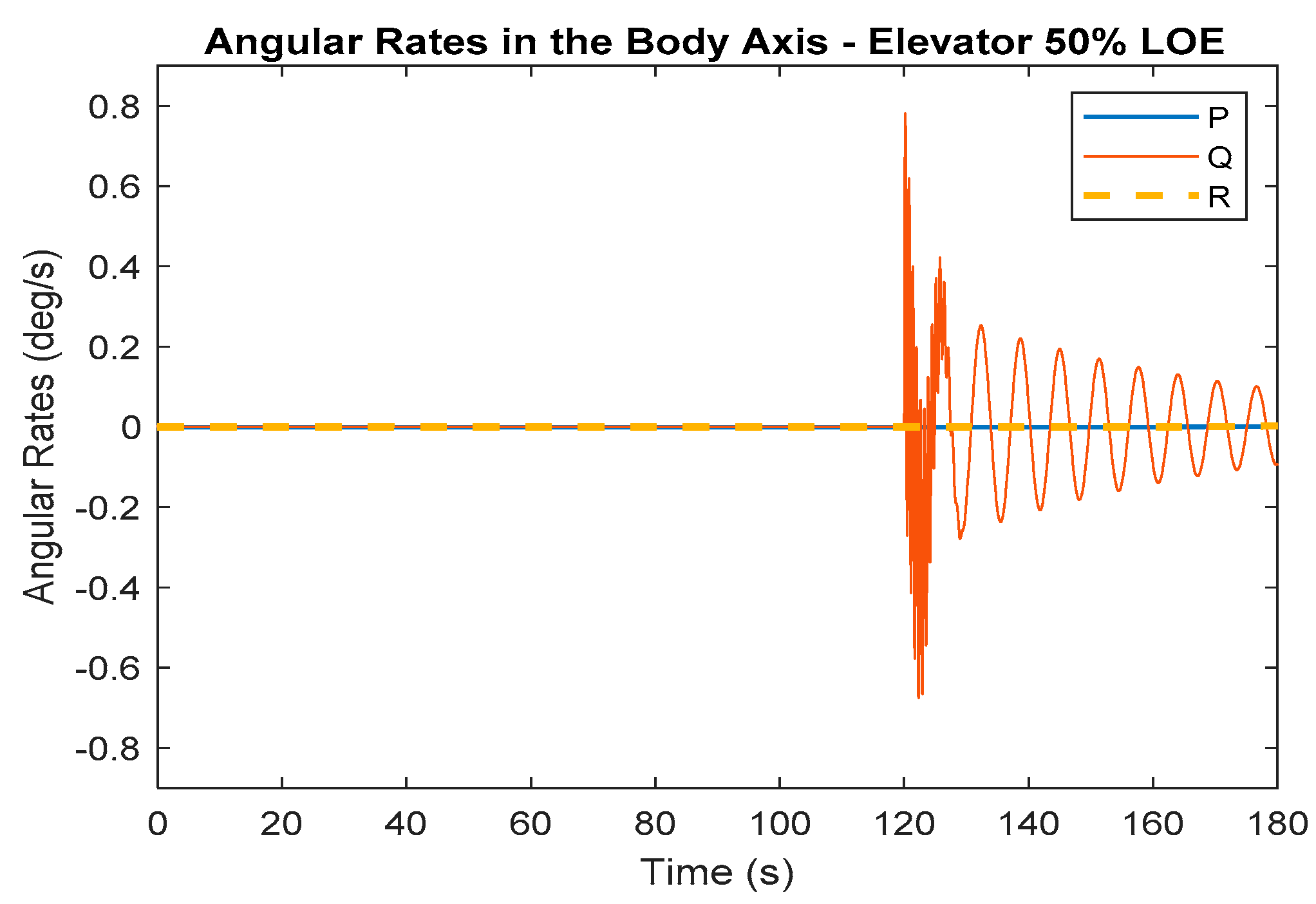
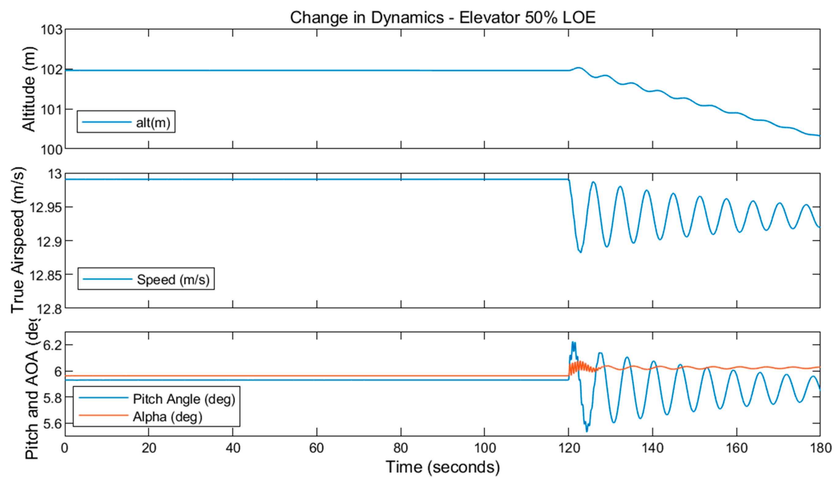
Figure 7 and Figure 8 below show the feature vector dataset variables plotted against time for the 50% LOE elevator actuator fault. Figure 9 shows the change in the SWIFT dynamics due to the fault. When the 50% LOE elevator fault occurs, the model starts to oscillate with a high frequency in the variables $q$, $a_x$, and $a_z$. Similar results are seen for the 25% and 75% LOE faults. These particular variables are more affected as they relate to the dynamics in the longitudinal motion and, therefore, vary as the fault in the elevator occurs.

The data from the feature vectors are labelled and split into the training and testing data. The performance of the trained SVM models is evaluated using the test data. The F1 score (which is derived from the confusion matrix) and the classification accuracy results are presented in

Table 3. Performance evaluation of the SVM models trained for the elevator actuator LOE fault.

	25% LOE—Elevator Actuator Fault	50% LOE—Elevator Actuator Fault	75% LOE—Elevator Actuator Fault
Confusion Matrix	$\left[\begin{array}{cc}501& 0\\ 0& 265\end{array}\right]$	$\left[\begin{array}{cc}491& 0\\ 0& 277\end{array}\right]$	$\left[\begin{array}{cc}507& 0\\ 0& 258\end{array}\right]$
F1 Score	1	1	1
Cross-Validation Classification Error	$3.14\times {10}^{-4}$	$3.26\times {10}^{-4}$	$3.23\times {10}^{-4}$

. The confusion matrix contains the number of true positives, false positives, true negatives, and false negatives and is arranged in a matrix as in [TP FP; FN TN]. The true positives are the number of data points the model has correctly classified as nominal, and the true negatives are the number of data points the model has correctly classified as faulty. The F1 score is derived from the confusion matrix values as shown in Equation (22). The SVM models trained for the 25% LOE fault, 50% LOE fault, and 75% LOE fault each scores a F1 score of one. This indicates that each model has perfectly classified the datapoints of the test data into the correct class: ‘nominal’ or ‘faulty’. A reason for this accuracy could be due to the change in the dynamic behaviour of the model for certain feature vectors when moving from a nominal actuator state to a faulty actuator state, as seen in Figure 7 and Figure 8.

Another performance metric measured is the cross-validation classification error. Cross-validation using the k-fold method is an important test as the results can be used to predict whether or not a model would be accurate in a real-world environment with new and dynamic data. The SVM models for the elevator LOE faults obtain a low cross-validation classification error. These results show that the misclassification rate for future out-of-sample data related to an elevator LOE fault is extremely low, giving an accuracy of 99.999%. This is a promising result.

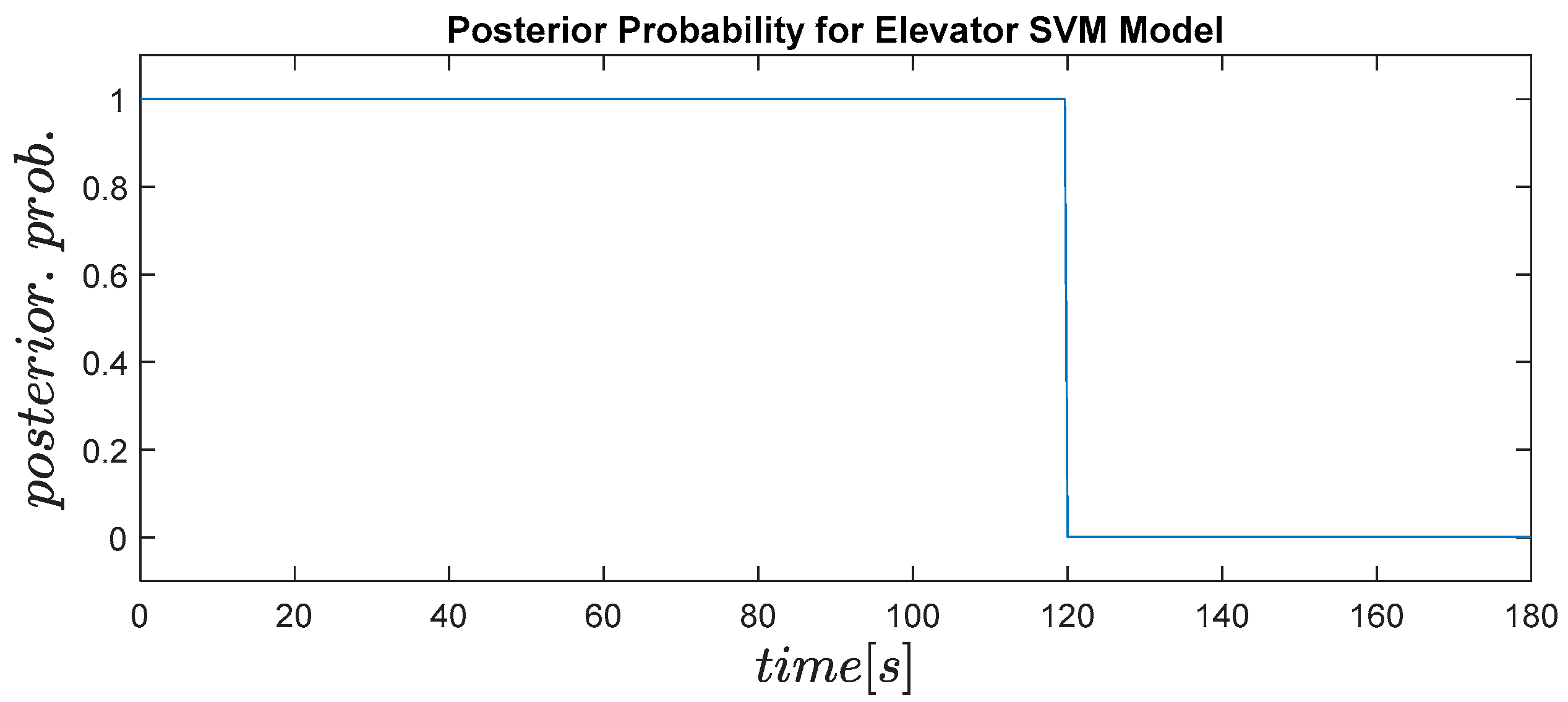
Not only does the model have to be accurate but it also must have a quick detection time so that corrective action could be applied. The posterior probability for the elevator actuator 50% LOE fault is plotted in Figure 10. In this plot, one represents the likelihood of the data being nominal and zero is the likelihood of the data being faulty. This plot shows the model instantly detects the fault at 120 s as the plot drops to zero. Similar results are seen for the other two percentages. In conclusion, the SVM models designed to detect elevator actuator LOE faults can detect faults instantly, with an accuracy of 100%.

4.3. SVM Model for Aileron Actuator LOE Fault

In this test, the elevator actuator is kept at its trim position, and a fault is injected into the aileron actuator in the same manner as for the elevator actuator. The aileron trim position in steady level flight is $0 \mathrm{deg}$. Three different percentages of LOE are investigated: 10%, 15%, and 20%.

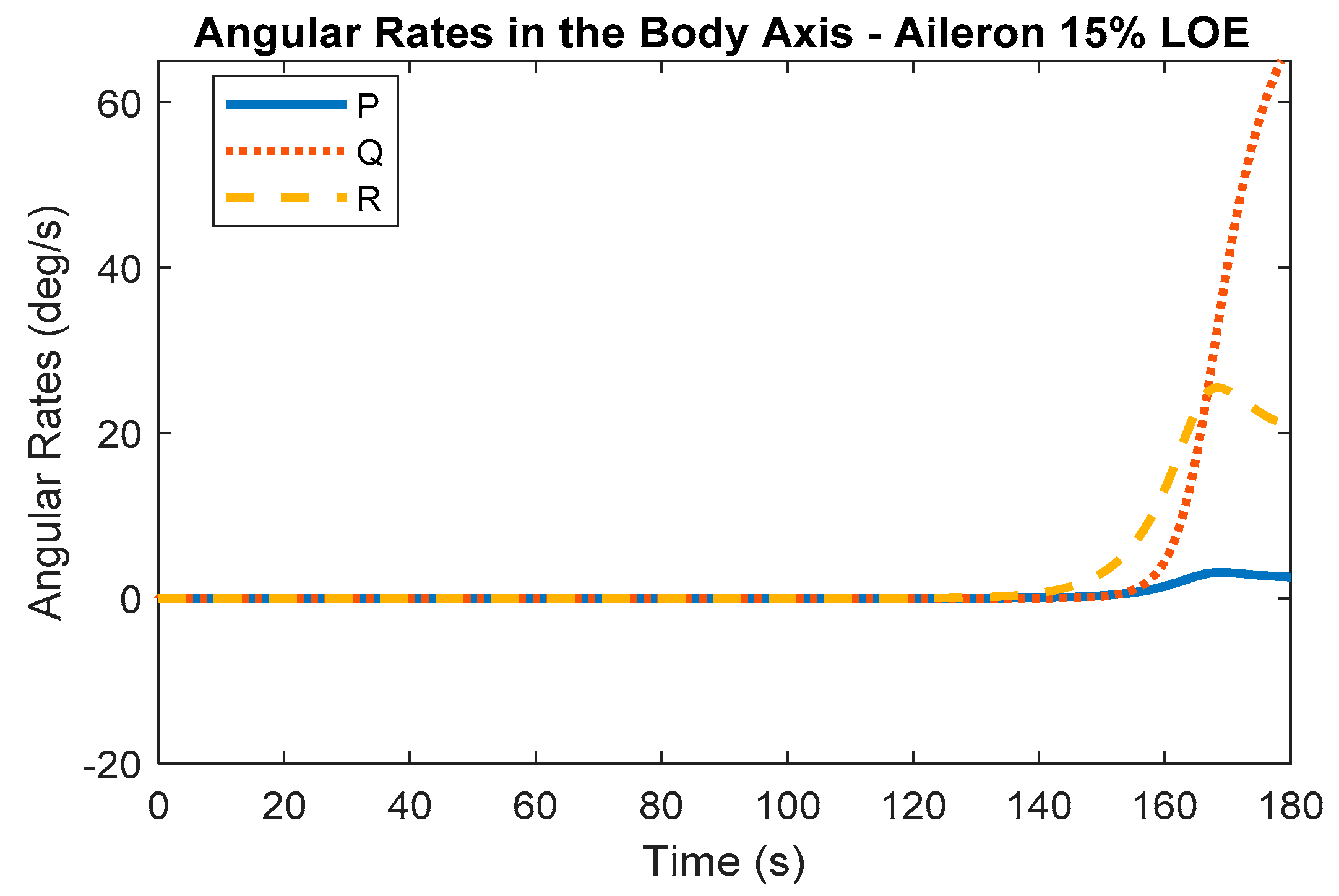
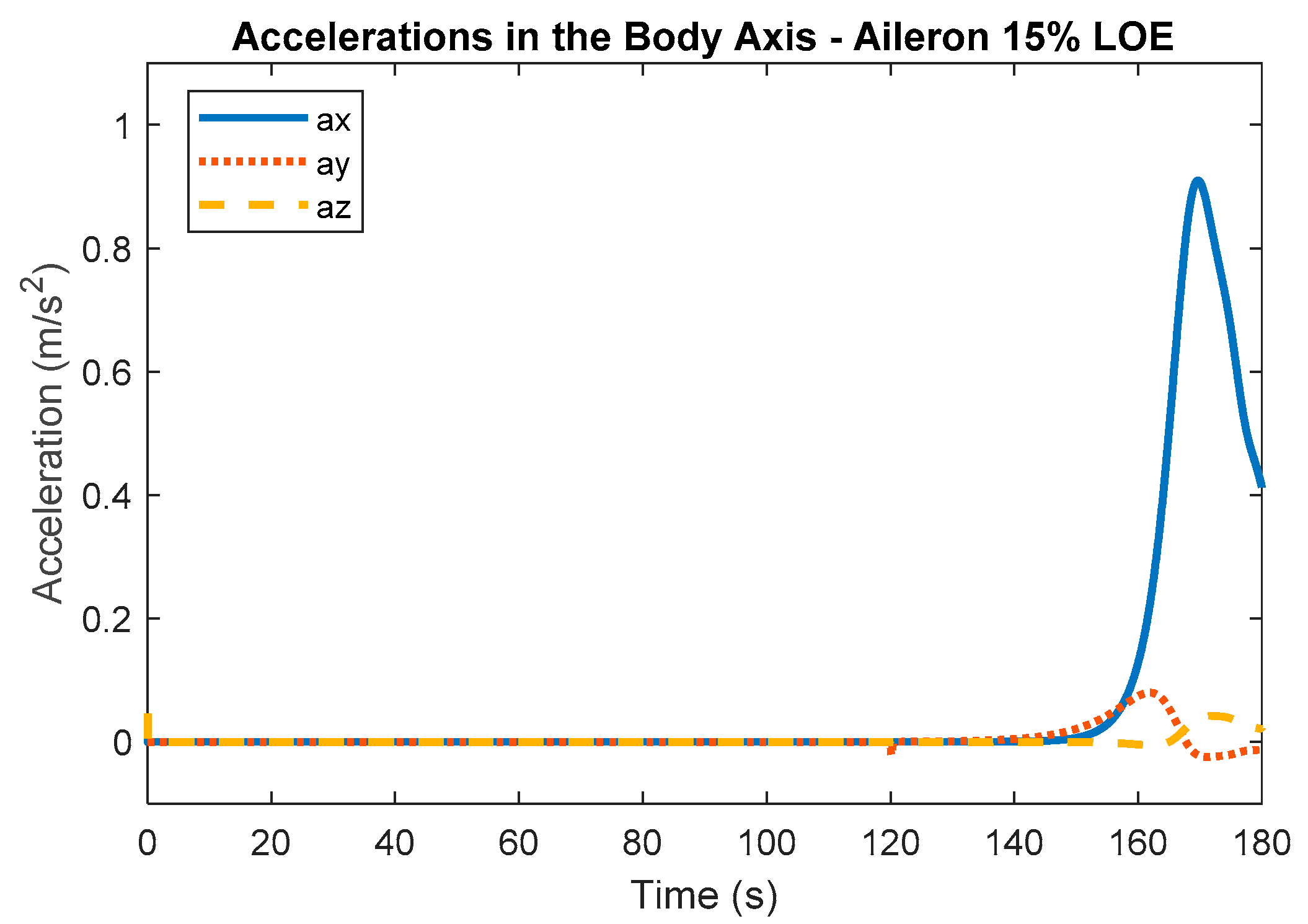
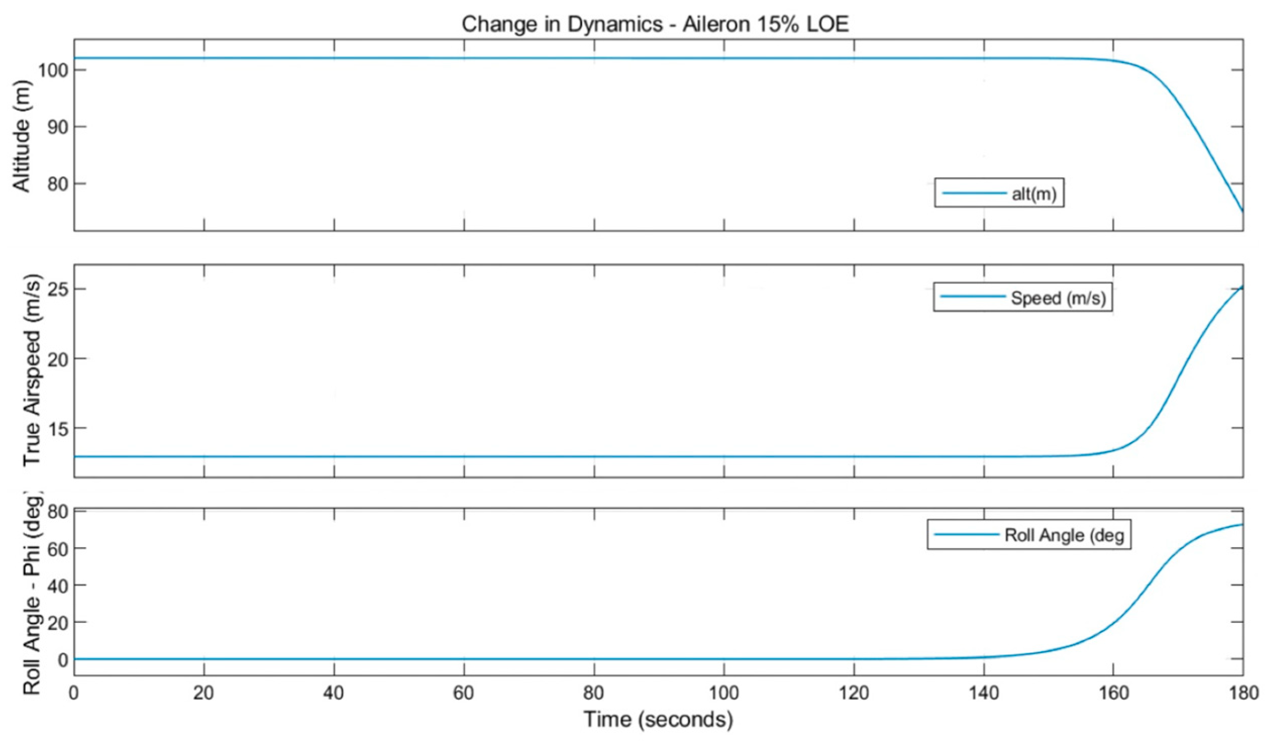
Figure 11 and Figure 12 show the feature vector dataset for the aileron 15% LOE fault. After the fault occurs, the variables show a steep increase. Figure 13 shows the change in dynamics due to the fault. In Figure 13, after the fault, the roll angle massively increases. This large increase due to the fault causes the aircraft to descend with an increasing speed, which causes instability in the system.

The SVM models are trained for each of the three percentages of LOE and evaluated, with the results shown in

Table 4. Untuned SVM aileron results for LOE fault detection.

	10% LOE Aileron Actuator Fault	15% LOE Aileron Actuator Fault	20% LOE Aileron Actuator Fault
Confusion Matrix	$\left[\begin{array}{cc}506& 58\\ 1& 245\end{array}\right]$	$\left[\begin{array}{cc}510& 45\\ 0& 270\end{array}\right]$	$\left[\begin{array}{cc}496& 45\\ 0& 296\end{array}\right]$
F1 Score	0.9439	0.9572	0.9565
Cross-Validation Error	0.0648	0.0539	0.04149
Hyperparameters:   $\sigma$  and  $C$	$\sigma =1$ $C=1$	$\sigma =1$ $C=1$	$\sigma =1$ $C=1$

. The aileron SVM model for each percentage performed is worse than the corresponding elevator SVM model. On average, 5% of data are misclassified across each of the three models. Each model also records a relatively high cross-validation error, meaning these models are more likely to incorrectly classify out-of-sample data.

Due to the slightly poorer performance of these aileron SVM models in comparison to the elevator SVM models, a tuning of the hyperparameters is performed. The models are tuned using Bayesian optimisation techniques, where the optimal values for the kernel scale, $\sigma$, and the box constraint, $C$, are obtained. The objective function model is seen in Figure 14a. In Figure 14b, it can be observed that the objective function model converges quickly after around five function iterations to the minimum point. The tuned hyperparameters are presented in the bottom row of

Table 5. Tuned SVM aileron results for LOE fault detection.

	10% LOE Aileron Actuator Fault	15% LOE Aileron Actuator Fault	20% LOE Aileron Actuator Fault
Confusion Matrix	$\left[\begin{array}{cc}506& 0\\ 1& 303\end{array}\right]$	$\left[\begin{array}{cc}490& 0\\ 0& 335\end{array}\right]$	$\left[\begin{array}{cc}496& 0\\ 0& 341\end{array}\right]$
F1 Score	0.9983	1	1
Cross-Validation Error	$6.1690\times {10}^{-4}$	$6.0533\times {10}^{-4}$	$5.9701\times {10}^{-4}$
Hyperparameters—$\sigma$ and $C$	$\sigma =0.00049$ $C=1399$	$\sigma =0.0045$ $C=1388$	$\sigma =0.00045$ $C=3894$

. For each of the models, the box constraint parameter increases, meaning that the margin of the hyperplane is smaller for the tuned models. The kernel scale defines how far the influence of a single point reaches the hyperplane. The kernel scale decreases, which implies that the region of influence for the support vectors, which shape the hyperplane, has increased to include more of the training set. The hyperparameters in the aileron LOE SVM models are fixed using the tuned parameters, and the models are retested. The same three results are recorded, as shown in Table 5, for the confusion matrix, the F1 score, and the cross-validation classification error. Due to this tuning of the hyperparameters, the accuracy of the model for each test case has increased by an average of 5%. The cross-validation classification error has also decreased by an average of 98%. This is a brilliant result and means that the tuned aileron SVM models are 98% more likely to classify out-of-sample data correctly and instantly than their untuned counterparts.

4.4. SVM Model for Elevator and Aileron Actuator LOE Faults

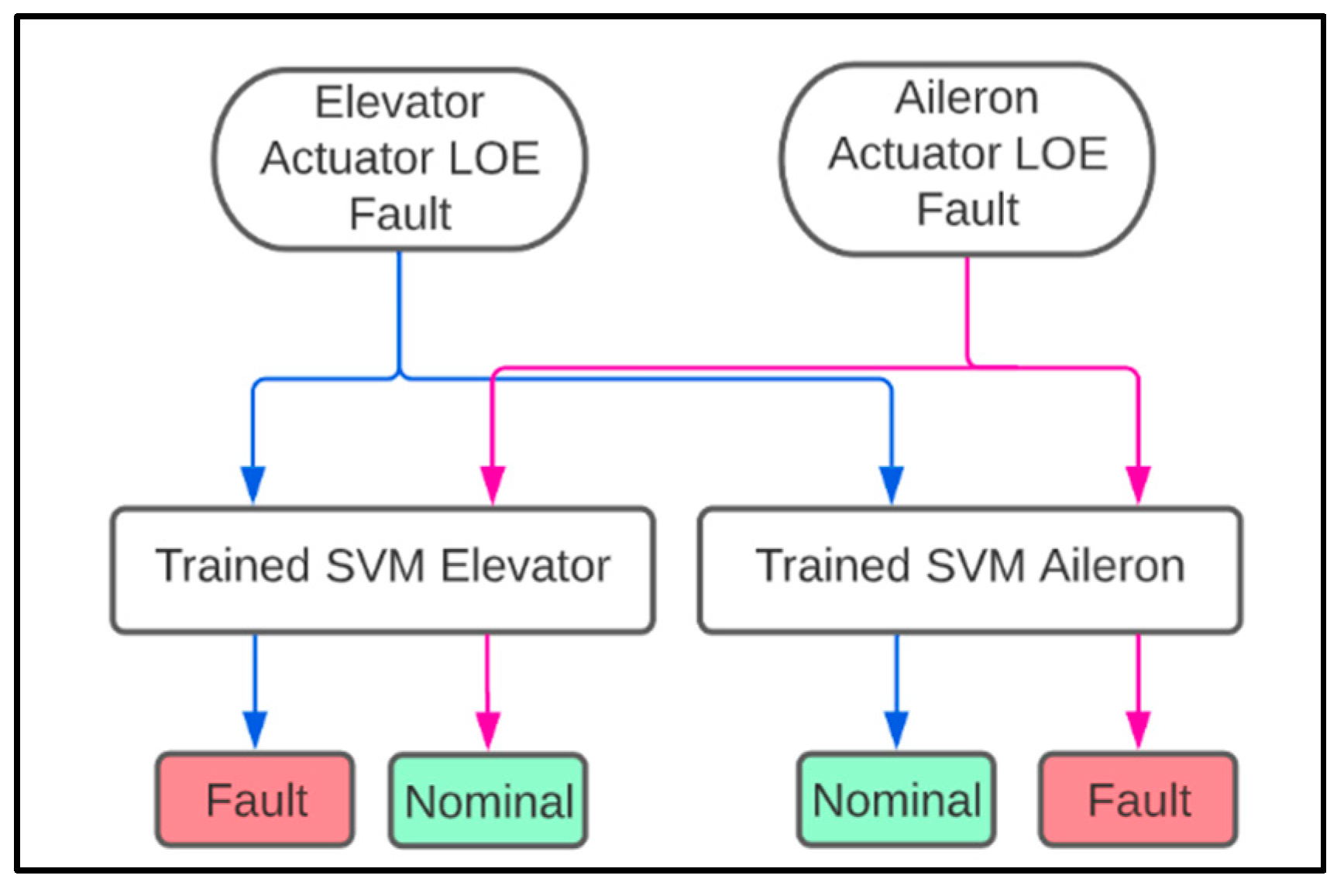
In the previous two sub-sections, the accuracy of the SVM models is evaluated separately for the elevator and aileron control surface LOE faults. In this section, an SVM model trained for elevator faults is tested with the feature vector data from the aileron faults. In a similar manner, the SVM model trained for aileron faults is tested with the feature vector data from the elevator faults. This is visualised in Figure 15 along with the expected results. The purpose of this test is to examine if there is any cross-correlation between the elevator and aileron SVM models. The hypothesis is that a SVM model trained for a certain actuator should not classify other actuator faulty data as faulty. If the elevator SVM model recognises the aileron faulty data as faulty, and vice versa, there is cross-correlation, and improvements to the models would be needed.

Firstly, the elevator SVM model trained for 50% LOE is tested using the output aileron data for 15% LOE. Secondly, the aileron model trained for 15% LOE is tested using the output data for the 50% elevator LOE fault.

From

Table 6. The results for the elevator SVM model trained for 50% LOE and tested with aileron data, and the results for the aileron SVM model trained for 15% LOE and tested with elevator data.

	Elevator SVM with Aileron Data	Aileron SVM with Elevator Data
Confusion Matrix	$\left[\begin{array}{cc}497& 0\\ 0& 328\end{array}\right]$	$\left[\begin{array}{cc}494& 1\\ 0& 274\end{array}\right]$
F1 Score	1	0.9989

, it is observed that the models perform well with high F1 scores. This is an extremely useful result, meaning that the model trained to detect one type of failure could detect another type of failure, which improves the detection capabilities of the system. However, the goal is not only to detect but also to isolate a fault. By referring to the definitions in the confusion matrix, it can be deduced that the FDI in the current form can detect a failure but cannot classify it correctly. The elevator SVM model has incorrectly classified aileron faults as elevators faults, and the aileron SVM model has incorrectly classified elevator actuator faults as aileron faults. The models do manage to classify the nominal data successfully, but further improvements are needed to classify elevator faults from aileron faults.

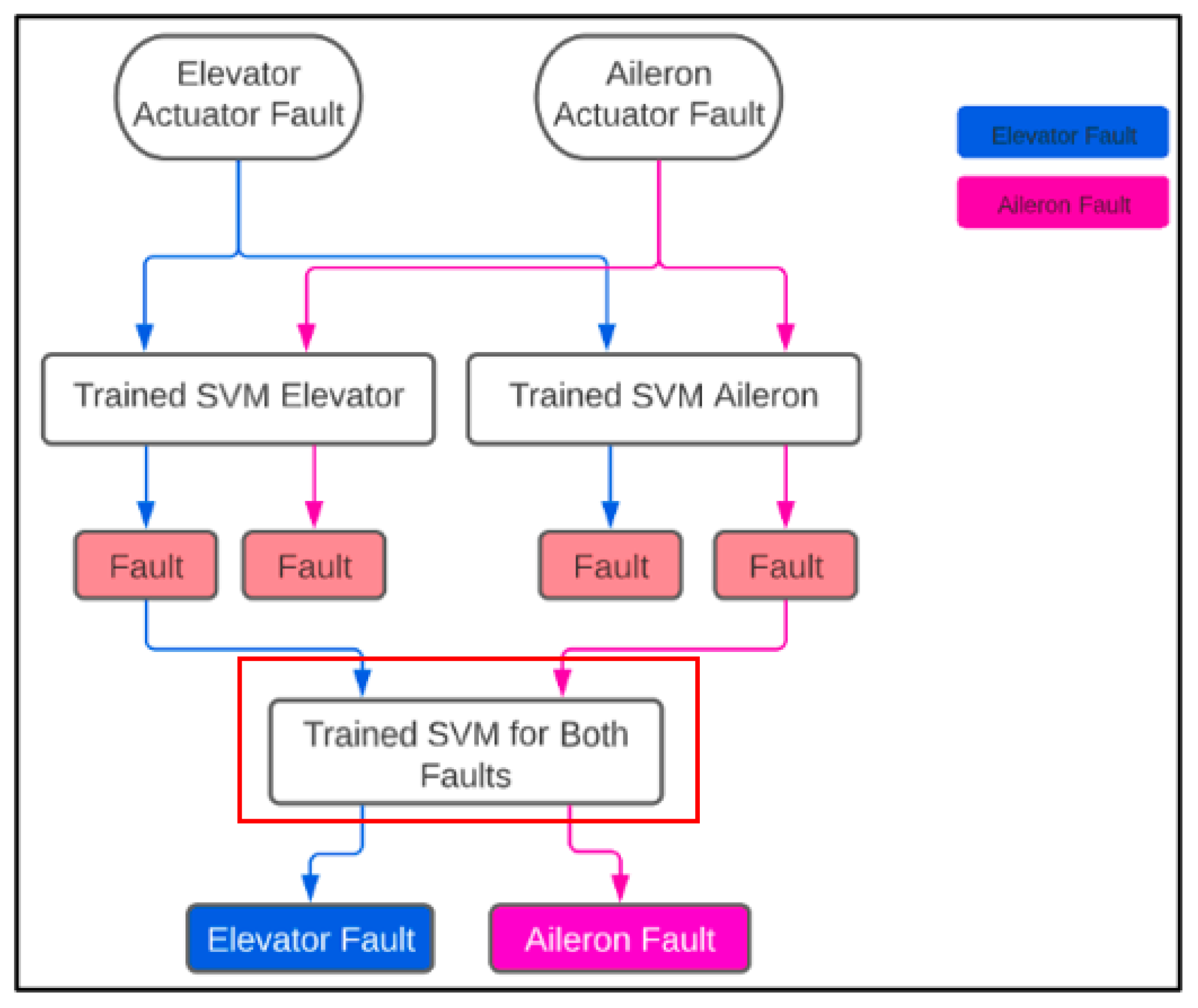
To rectify this issue, another SVM model is trained, and this additional model is shown in Figure 16. The purpose of this SVM model is to try to classify the “fault” data from the SVM elevator and SVM aileron models into “elevator fault” or “aileron fault” as the previous models could only detect “fault”. The additional model is shown by the red box. The additional model is first trained using both the 60 s of the elevator faulty data and the 60 s of the aileron faulty data. The output of the SVM model trained for both types of faults is now “Elevator Fault” or “Aileron Fault”.

The results for the model tuned for both types of faults are recorded in

Table 7. SVM results for model trained for both types of faults—tuned and untuned.

	SVM Model for Both Faults—Untuned	SVM Model for Both Faults—Tuned
Confusion Matrix	$\left[\begin{array}{cc}266& 47\\ 0& 272\end{array}\right]$	$\left[\begin{array}{cc}266& 1\\ 0& 318\end{array}\right]$
F1 Score	0.9188	0.9989
Cross-Validation Error	0.0781	0.0029
Hyperparameters—$\sigma$  and  $C$	$\sigma =1$ $C=1$	$\sigma =0.02069$ $C=95054$

. In this confusion matrix for the SVM model trained for both types of faults, the definitions change and are as follows:

• True Positive: Model classifies an elevator fault as an elevator fault.
• True Negative: Model classifies an aileron fault as an aileron fault.
• False Positive: Model classifies an aileron fault as an elevator fault.
• False Negative: Model classifies an elevator fault as an aileron fault.

The untuned SVM model for both types of faults has 47 false positives (from the total 585), where the model classifies an aileron fault as an elevator fault. The untuned model also has a poor cross-validation error in comparison to the previous models that are trained for singular faults. To improve the accuracy of the model, the hyperparameters are tuned using Bayesian optimisation techniques. The values for the hyperparameters are shown in Table 7. Like the aileron SVM model tuning, the box constraint parameter increases, and the kernel scale decreases. The tuning generates better results, with just one aileron fault being classified as an elevator fault. This misclassification could be rectified by using a larger training set with fault data greater than 60 s. However, overall, the F1 score improves 8% to 0.9989, which is a good result. The addition of another SVM model trained for both types of faults has successfully fixed the issue of cross-correlation, and the health monitoring system can detect and isolate aileron and elevator faults with 99.9% accuracy.

4.5. SVM Model for Elevator Actuator with Noisy Measurements

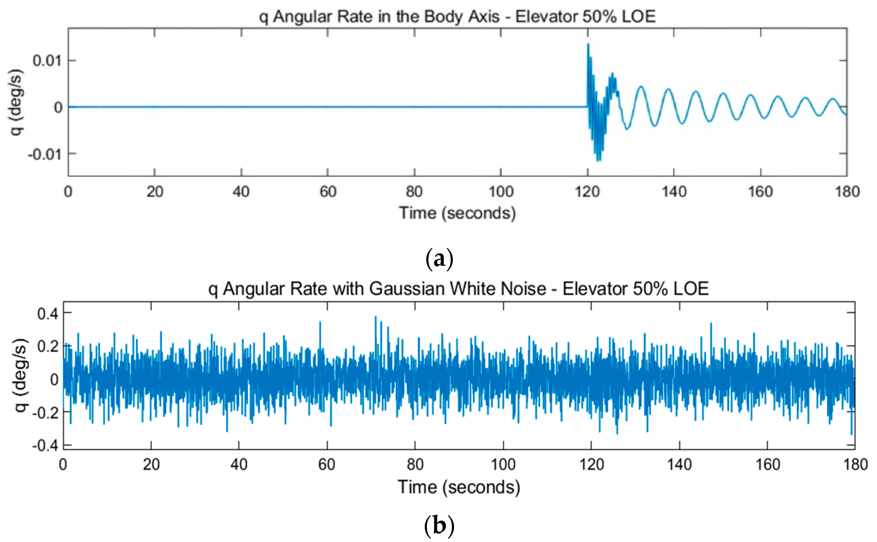
All real measurements are affected by noise. Mitigating the effects of noise in aircraft fault diagnosis methods is important as noise can cause a model to misclassify data. To investigate if the SVM model can handle noise, the following test is performed with the dataset for the 50% LOE elevator actuator fault. Gaussian white noise blocks are introduced to each output of the feature vector variables: $a_x,a_y,a_z,p,q,\mathrm{and} r$ in Simulink. The signal-to-noise ratio (SNR) in the block is set to $20 \mathrm{dB}$.

Figure 17 represents the plot of the feature vector variable, $q$, with (a) no noise and (b) noise. The results for the performance of the model are shown in

Table 8. SVM elevator actuator model results for Gaussian white noise with SNR of 20 dB.

	(a) Untuned + No Signal Filtering	(b) Untuned + Signal Filtering	(c) Tuned + Signal Filtering
Confusion Matrix	$\left[\begin{array}{cc}75& 3\\ 177& 513\end{array}\right]$	$\left[\begin{array}{cc}466& 50\\ 37& 215\end{array}\right]$	$\left[\begin{array}{cc}501& 0\\ 2& 265\end{array}\right]$
F1 Score	0.4545	0.9146	0.9979
Cross-Validation Classification Error	$0.2415$	0.1064	0.00423

. First, the feature vector data with the added noise and no filtering are labelled and split into the training and test data. The results of the model are poor and give the lowest F1 score obtained in all tests so far, with a value of 0.45. This is a bad result, and the model is shown to not be robust against noise. However, it is a common practice in machine-learning models to filter noisy signal data before using the data to train a model. The moving mean filter is a simple low-pass filter used for smoothing data. This filter is applied to each variable in the feature vector dataset by using the MATLAB function movmean.

The results improve significantly by using the moving mean filter. The smoothing technique allows the important patterns in the dataset to become visible to the SVM model, while leaving out the noise. The F1 score improves by just over 50%, and the classification error drops by a sizable 55%. In order to further improve the accuracy and robustness of this elevator SVM model, the hyperparameters of the model, $\sigma$ and $C,$ can be tuned. As in previous tests, the Bayesian optimisation method is used. The accuracy of the model again increases to an F1 score of 0.99, which is the best result for F1 score in Table 8. The accuracy of the tuned model with feature vector signal filtering is a clear improvement from the model that is untuned and employs no signal filtering. In conclusion, the robustness of the model against noise is considerably increased thanks to the moving mean filter and tuning of the hyperparameters.

4.6. SVM Model for Elevator Actuator in a Closed-Loop System

A basic longitudinal flight controller is designed for the SWIFT VTOL aircraft to see how the SVM actuator health monitoring system performs in a closed-loop system and to evaluate the interaction between FDI and the control system. The controller provides optimally designed feedback gain, $K$, for the elevator control input to enable closed-loop stability. In order to design the longitudinal controller, the SWIFT VTOL aircraft is trimmed at a different trim point, and the model is linearised. This leads to a changed elevator input angle of ${\delta }_{ele}=-10.824°$. The longitudinal state-space model is then extracted from the linearised model by selecting the states $u, w, q,$ and $\theta$. Values for $Q$ and $R$ are chosen, and the function lqr is used. The controller gain $K$ is then saved and imported into the full model.

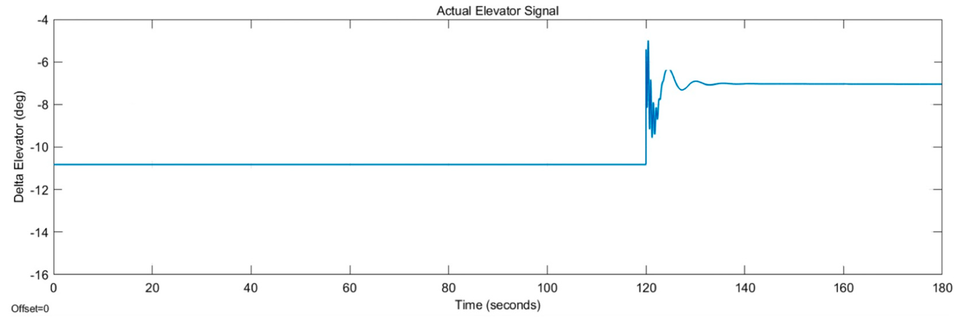
The fault investigated for this section is the 50% LOE fault in the elevator actuator. The simulation runs for the same time as other tests, for $180 \mathrm{s},$ and the LOE fault is injected into the system at $120 \mathrm{s}$. By observing the actual elevator input signal in Figure 18, it can be seen that the fault occurs and is controlled for about 20 s between 120 and 140 s. The fault initially causes a high-frequency oscillatory response in the control signal. This response is a result of the controller working to stabilise the system. After 140 s, the controller is able to compensate for the actuator fault. In the basic LQR design, the controller does not compare the output elevator actuator signal to the reference; it instead compares all of the states multiplied by the control matrix to the reference. Therefore, it is not always expected that the output equals the commanded reference with the design, and there will be a steady-state error. However, the controller is still capable of compensating for the fault and stabilising the system.

The results for the elevator SVM model for a closed-loop system are presented in

Table 9. Closed-loop elevator SVM model results with tuned hyperparameters.

	Elevator SVM Model for a Closed-Loop System
Confusion Matrix	$\left[\begin{array}{cc}360& 1\\ 0& 178\end{array}\right]$
F1 Score	0.9989
Cross-Validation Error	$10.23\times {10}^{-3}$
Hyperparameters—$\sigma$  and  $C$	$\sigma =0.000025$ $C=895$

. The tuning reduces the cross-validation error significantly by 96% and increases the F1 score by an average of 16%. The tuned model has a low kernel scale of 0.000025 and a higher box constraint of 895, which follows the tuned hyperparameter trend seen in open-loop systems.

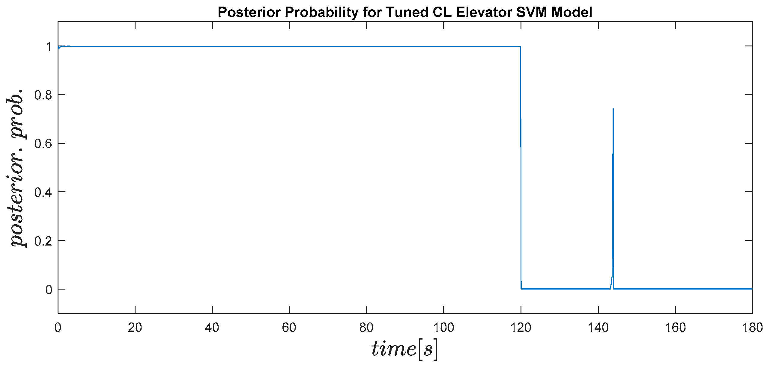
In Figure 19, the posterior probability plotted against time for the tuned closed-loop elevator SVM model can be seen. The probability of the data being classed as nominal is one, and for being classified as faulty, it is zero. The model instantly detects the fault at 120 s. However, the spike in the faulty data at 145 s is result of the model misclassifying the likelihood of the data as being faulty. This spike is observed in the confusion matrix at the one point that is a false positive, meaning the model has classified a faulty situation as nominal. Overall, the tuned SVM model for elevator within the closed-loop system performs well and provides similar accuracy to that of the OL model with the tuned parameters, giving 99% accuracy.

In order to prove the importance of this closed-loop fault detection SVM model, the following test is performed: classify closed-loop feature vector data using an open-loop model for the elevator actuator 50% LOE fault. The results are shown in

Table 10. Elevator SVM model trained for an open-loop system and tested with closed-loop data.

	OL Elevator SVM Model Tested with CL Data—50% LOE Fault
Confusion Matrix	$\left[\begin{array}{cc}365& 118\\ 0& 56\end{array}\right]$
F1 Score	0.86

. The model achieves a low F1 score of 0.86. The model records 118 false positives, which means that the model has classified 118 faulty data points as nominal. A false positive result is pointed out as the worst error that a SVM model could produce. This test validates the importance of closed-loop fault detection. By using the elevator model trained for closed-loop fault detection for real flight data, the accuracy should be better by 13%. This is a significant result considering how important accurately classifying actuator faults is for ensuring flight reliability.

5. Discussion and Conclusions

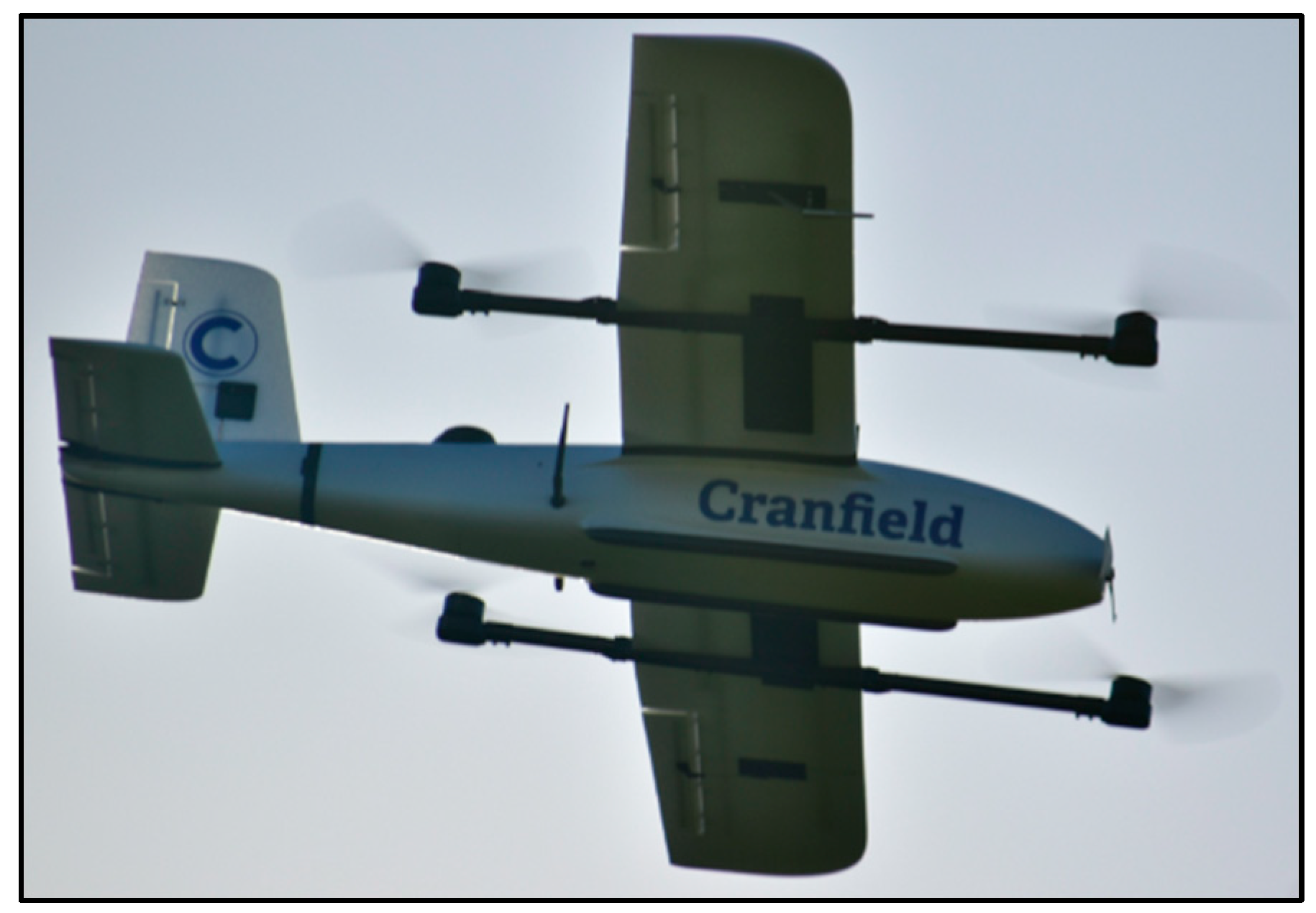
In this paper, a data-driven fault diagnosis method to detect and identify faults in an aircraft flight control actuation system is developed. To develop the data-driven algorithm, a non-linear aircraft model is needed to provide simulated flight data. The aircraft chosen was the SWIFT VTOL. A model of the SWIFT aircraft with actuator fault modes was created in Simulink. The actuator fault investigated in this study was the loss-of-effectiveness (LOE) fault, which was simulated by applying a gain to the control signal at the fault time. This model was successful in providing flight data in an open-loop system. To study the effects of the flight controller on the fault diagnosis algorithm, an LQR controller was designed and implemented in the SWIFT VTOL Simulink to provide closed-loop flight data.

Once the model was completed, a fault diagnosis algorithm was developed. A Support Vector Machine algorithm was the chosen method, as SVM had shown promising results in classifying aircraft actuator failures. The algorithm was developed in MATLAB. The input to the SVM model was the labelled feature vector data from the SWIFT VTOL model. This data consisted of the signal output values of the body acceleration in each axis and the body angular rates. Several tests were performed that included injecting faults into the aileron and elevator actuators. The aim of the fault detection algorithm was to classify the feature vector data into a nominal or a faulty class. The elevator SVM models classified the LOE faults instantly, scoring an F1 score of one. The tuned aileron SVM models also showed great accuracy, with the models scoring an average F1 score of 0.99. The models for each control surface also showed a low cross-validation classification error for the out-of-sample data, with values of ${10}^{-4}$. This is a very promising result, with the models showing a satisfactory performance.

This study manifested a tremendous effect of the sensor noise on the classification precision. The baseline system was not robust against the sensor noise. However, by adding a simple low-pass filter into the framework, this issue could be tackled, and the performance was significantly improved. By using the filter and tuning the model, it kept a high F1 score of 0.99.

During the test phase, the cross-correlation between the models was also investigated. It was shown that the elevator SVM model detected aileron actuator faults. This by-product result showed that the SVM model trained to detect one type of failure could detect another type of failure, showing good generalisation capabilities. Nevertheless, the goal was not only to detect but also to isolate a fault. To improve isolation capabilities, an additional model was trained that could detect the difference between elevator and aileron actuator faults. This model performed well when tuned and gave an accuracy of 99%. This method could be improved by creating a multi-class SVM model. However, multi-class models have been shown to be slower during the training phase than binary SVM models.

It was demonstrated that the interaction of the proposed SVM-based FDI with the control system could mislead the classification. The open-loop elevator SVM model was tested with the closed-loop data. The model scored a low F1 score of 0.86, and the accuracy dropped 13% in comparison to the closed-loop model. However, the SVM model trained with the faulty closed-loop system data scored an F1 score of 0.99, which was on par with the open-loop results. Fault detection algorithms based on Support Vector Machines were developed for the elevator and aileron actuators. These algorithms could detect the LOE fault instantly, with an average of 99% accuracy. These results are in line with those achieved in [25], in which an F1 score of 0.99 was also achieved when testing an optimised SVM model on its ability to detect flight control actuation faults.

It is noted that the fault detection algorithm developed in this paper is limited to detecting the loss-of effectiveness actuator fault. Future research could be centered around developing a multi-class SVM model to detect multiple faults for each of the primary aircraft control surface actuators. This is a complicated process due to the multiple different faults that can occur, but with sufficient training, a multi-class model should be capable of detecting different types of faults to a good accuracy. It is also noted that the work presented here is limited by the use of simulated flight data from the SWIFT VTOL model. Future work should test this fault detection algorithm on data captured from real drone flight tests to increase the robustness of this FD algorithm. Such additional research would test the algorithm and highlight any potential strong points (such as the ability to handle noisy measurements) or areas that could require more model training (fault detection in a closed-loop system).

To conclude, fault detection algorithms based on Support Vector Machine were developed for the elevator and aileron actuators. These algorithms can detect the LOE fault instantly, with an average accuracy of 99%. Overall, the proposed SVM-based FDI framework demonstrates promising fault classification capabilities, which might be utilised in integrated FDI and reconfigurable flight control systems to advance pilot-based health-monitoring to an autonomous health-management system and enable future pilotless UAS systems.