
Formation Control for Second-Order Multi-Agent Systems with Collision Avoidance


Abstract
1. Introduction
2. Preliminaries
2.1. Graph Theory
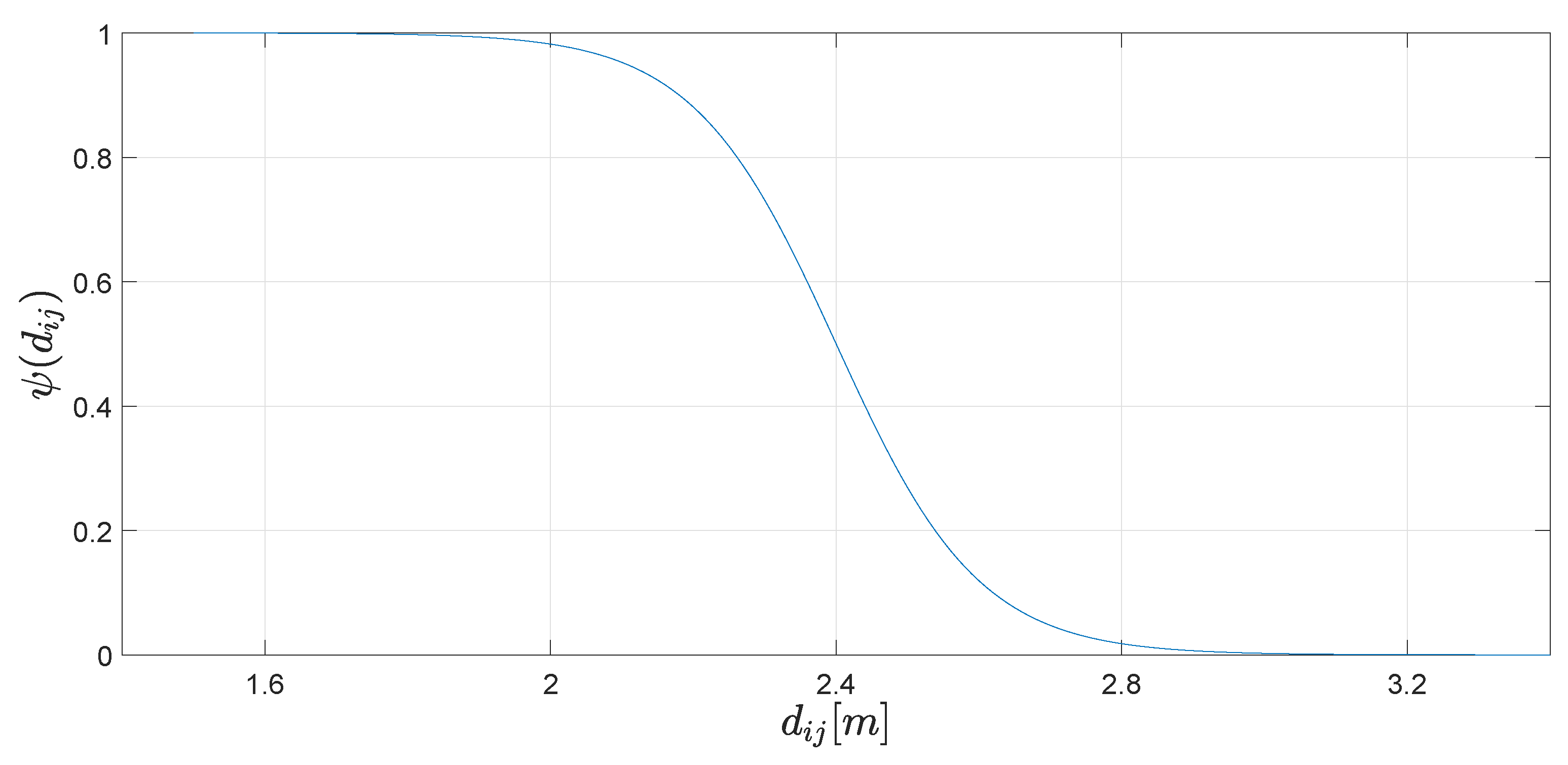
2.2. Saturating and Switching Functions
- ;
- for some ;
- , ;
- .
- if ;
- if ;
- if ;
- .
2.3. Input-to-State Stability
3. Problem Statement
3.1. Control Objective
- (i)
- The agents reach the desired relative positions, that is,
- (ii)
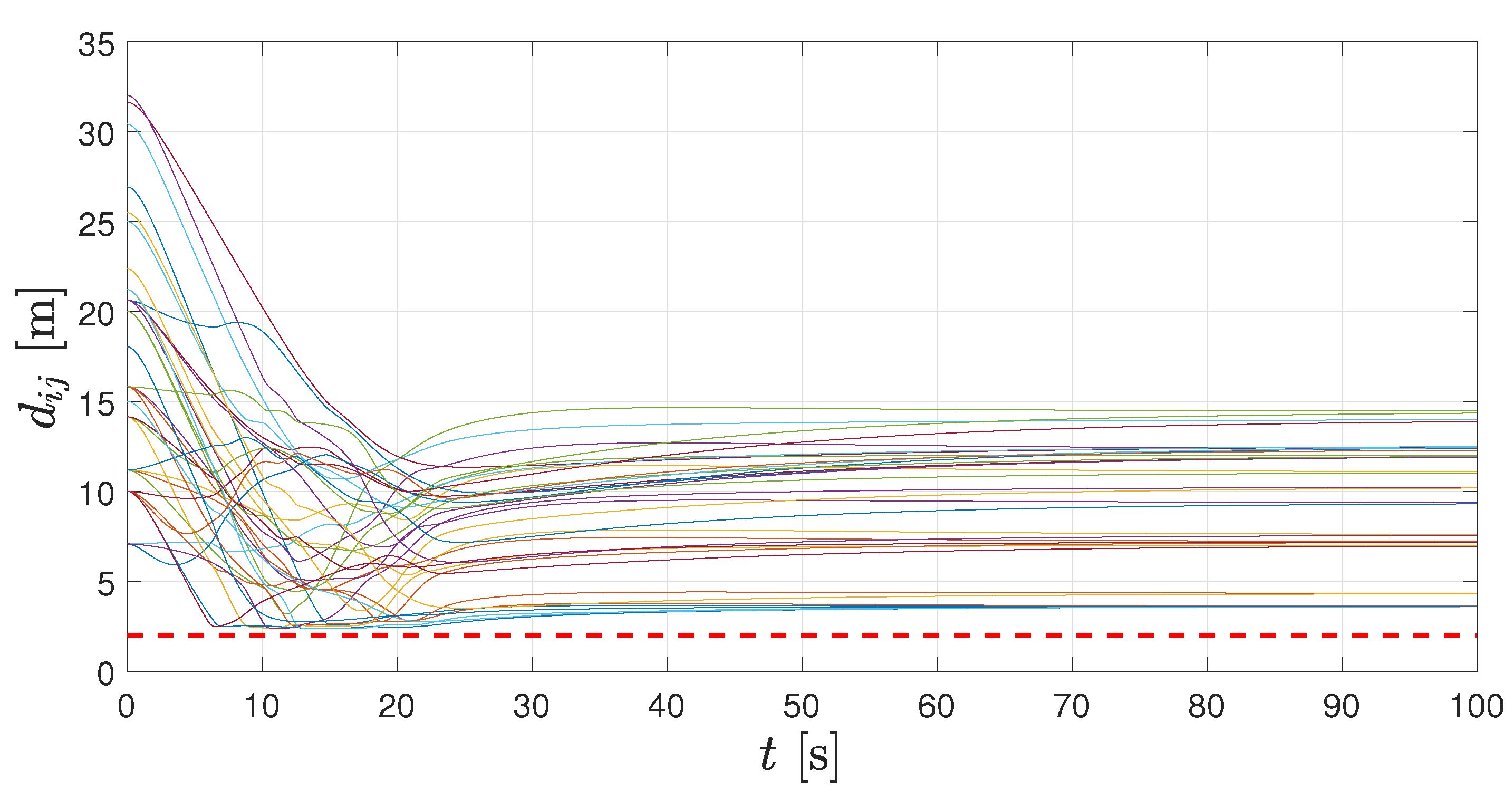
- There are no collisions among agents. Even more, the agents remain at some predefined distance d from each other, that is, , , ;
- (iii)
- Once the agents achieve the desired formation, the geometrical pattern does not move from its current location any more, i. e., , .
3.2. Position Error Dynamics
4. Control Design
4.1. Formation Control Strategy
4.2. Formation Control Strategy with Collision Avoidance
4.3. Reduced System
4.4. General System
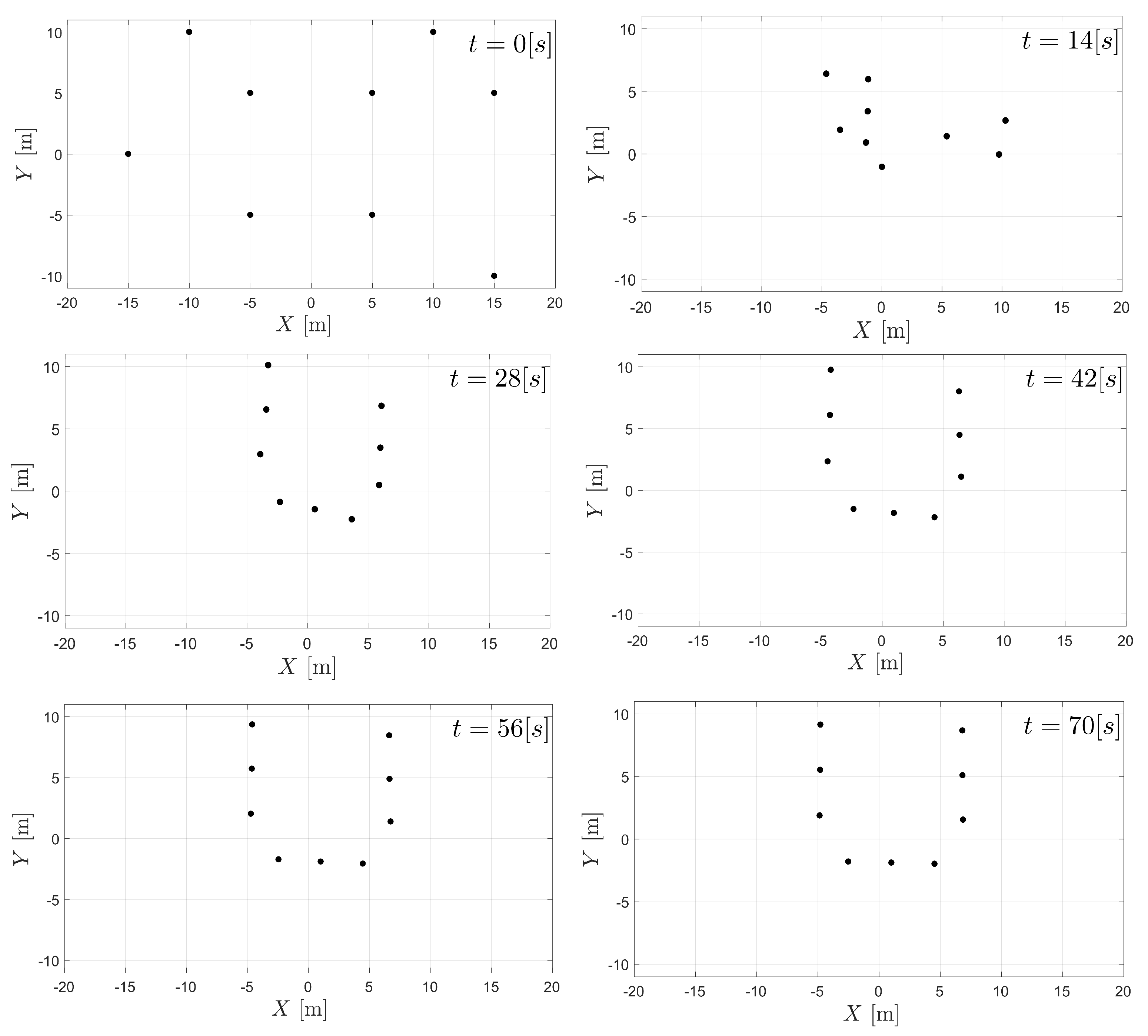
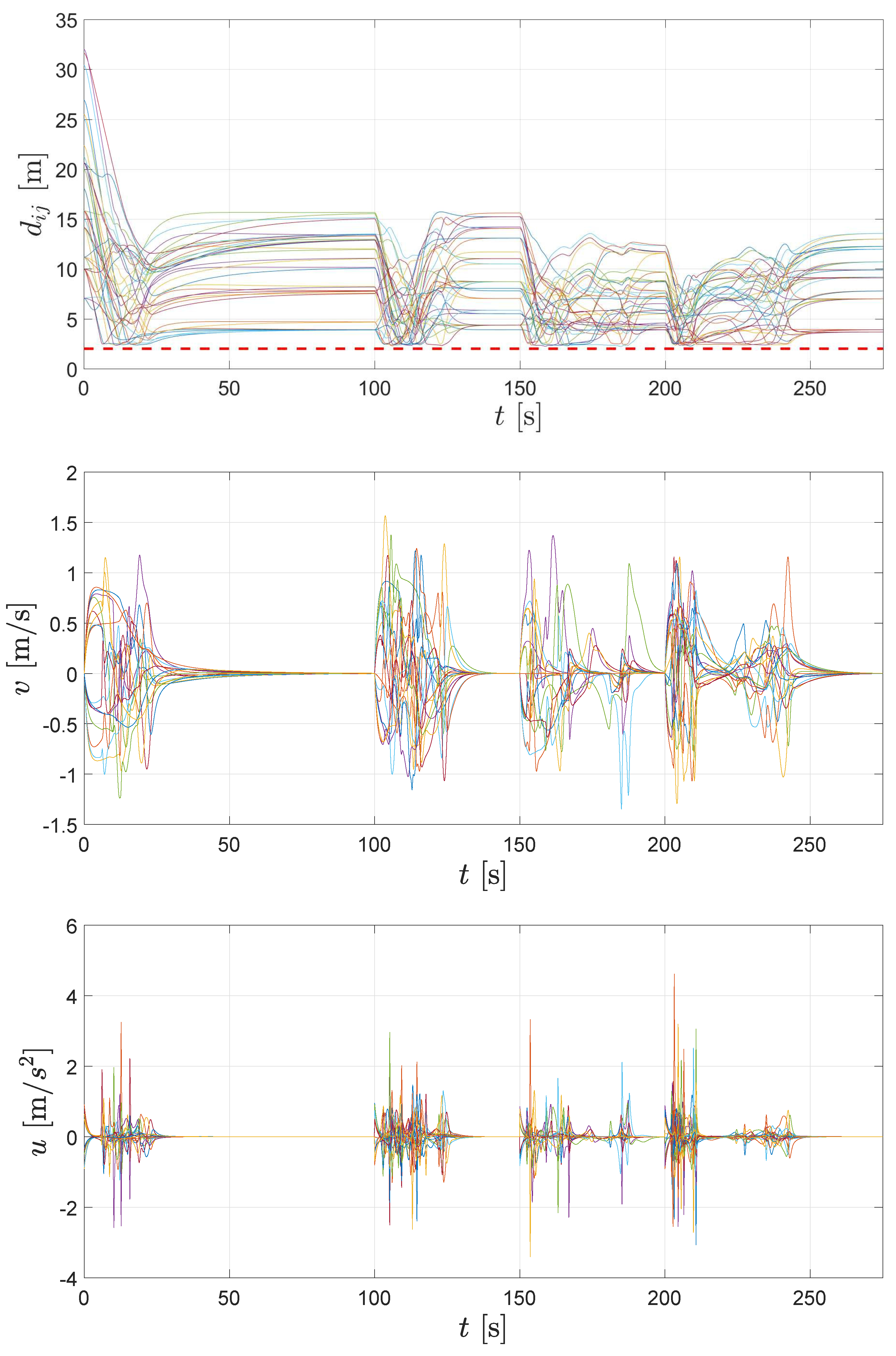
5. Simulations
5.1. Desired Formations
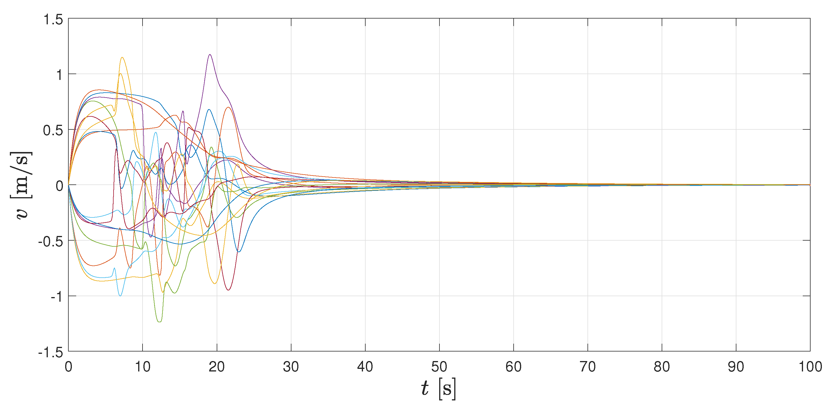
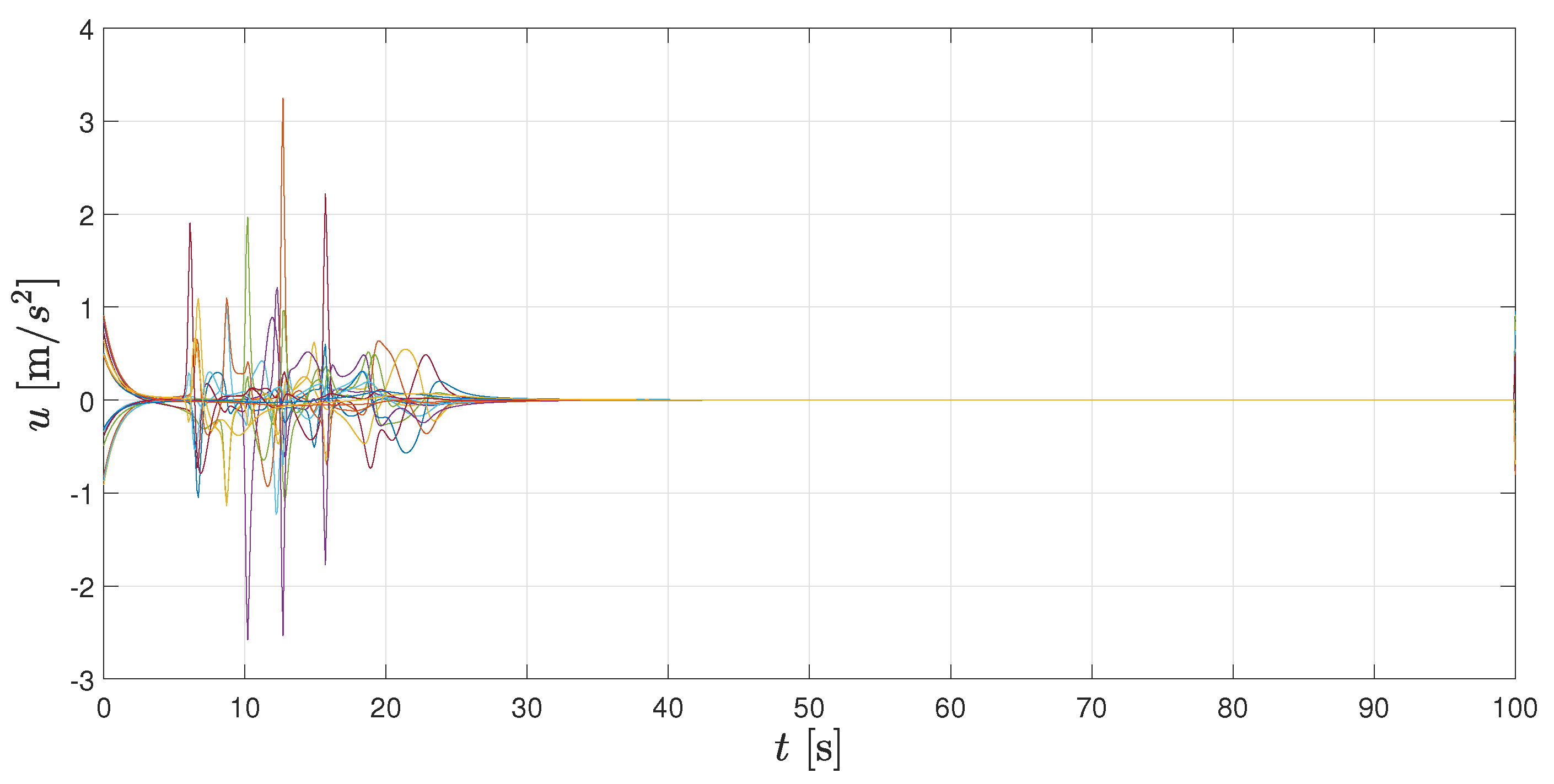
5.2. Simulation Results and Discussions
6. Conclusions
Supplementary Materials
Author Contributions
Funding
Data Availability Statement
Conflicts of Interest
Abbreviations
| ISS | Input-to-State Stable |
| GAS | Globally Asymptotically Stable |
References
- Ku, S.Y.; Nejat, G.; Benhabib, B. Wilderness Search for Lost Persons Using a Multimodal Aerial-Terrestrial Robot Team. Robotics 2022, 11, 64. [Google Scholar] [CrossRef]
- Nordin, M.H.; Sharma, S.; Khan, A.; Gianni, M.; Rajendran, S.; Sutton, R. Collaborative Unmanned Vehicles for Inspection, Maintenance, and Repairs of Offshore Wind Turbines. Drones 2022, 6, 137. [Google Scholar] [CrossRef]
- Sharma, M.; Gupta, A.; Gupta, S.K.; Alsamhi, S.H.; Shvetsov, A.V. Survey on Unmanned Aerial Vehicle for Mars Exploration: Deployment Use Case. Drones 2022, 6, 4. [Google Scholar] [CrossRef]
- Xie, J.; Liu, C.C. Multi-agent systems and their applications. J. Int. Counc. Electr. Eng. 2017, 7, 188–197. [Google Scholar] [CrossRef]
- Roldán-Gómez, J.J.; González-Gironda, E.; Barrientos, A. A Survey on Robotic Technologies for Forest Firefighting: Applying Drone Swarms to Improve Firefighters’ Efficiency and Safety. Appl. Sci. 2021, 11, 363. [Google Scholar] [CrossRef]
- Mondal, A.; Bhowmick, C.; Behera, L.; Jamshidi, M. Trajectory Tracking by Multiple Agents in Formation With Collision Avoidance and Connectivity Assurance. IEEE Syst. J. 2018, 12, 2449–2460. [Google Scholar] [CrossRef]
- Oh, K.K.; Park, M.C.; Ahn, H.S. A survey of multi-agent formation control. Automatica 2015, 53, 424–440. [Google Scholar] [CrossRef]
- Wu, S.; Pu, Z.; Yi, J.; Sun, J.; Xiong, T.; Qiu, T. Adaptive Flocking of Multi-Agent Systems with Uncertain Nonlinear Dynamics and Unknown Disturbances Using Neural Networks*. In Proceedings of the 2020 IEEE 16th International Conference on Automation Science and Engineering (CASE), Hong Kong, China, 20–21 August 2020; pp. 1090–1095. [Google Scholar] [CrossRef]
- Young, Z.; La, H.M. Consensus, cooperative learning, and flocking for multiagent predator avoidance. Int. J. Adv. Robot. Syst. 2020, 17, 1729881420960342. [Google Scholar] [CrossRef]
- Briñón-Arranz, L.; Seuret, A.; Canudas-de Wit, C. Cooperative Control Design for Time-Varying Formations of Multi-Agent Systems. IEEE Trans. Autom. Control 2014, 59, 2283–2288. [Google Scholar] [CrossRef]
- Ren, W.; Atkins, E. Distributed multi-vehicle coordinated control via local information exchange. Int. J. Robust Nonlinear Control 2007, 17, 1002–1033. [Google Scholar] [CrossRef]
- Dong, W.; Farrell, J.A. Cooperative Control of Multiple Nonholonomic Mobile Agents. IEEE Trans. Autom. Control 2008, 53, 1434–1448. [Google Scholar] [CrossRef]
- Do, K.; Pan, J. Nonlinear formation control of unicycle-type mobile robots. Robot. Auton. Syst. 2007, 55, 191–204. [Google Scholar] [CrossRef]
- Wen, G.; Duan, Z.; Ren, W.; Chen, G. Distributed consensus of multi-agent systems with general linear node dynamics and intermittent communications. Int. J. Robust Nonlinear Control 2014, 24, 2438–2457. [Google Scholar] [CrossRef]
- Anderson, B.D.O.; Sun, Z.; Sugie, T.; Azuma, S.; Sakurama, K. Distance-based rigid formation control with signed area constraints. In Proceedings of the 2017 IEEE 56th Annual Conference on Decision and Control (CDC), Melbourne, VIC, Australia, 12–15 December 2017; pp. 2830–2835. [Google Scholar] [CrossRef]
- Hernandez-Martinez, E.G.; Ferreira-Vazquez, E.D.; Fernandez-Anaya, G.; Flores-Godoy, J.J. Formation Tracking of Heterogeneous Mobile Agents Using Distance and Area Constraints. Complexity 2017, 2017, 13. [Google Scholar] [CrossRef]
- Mehdifar, F.; Bechlioulis, C.P.; Hashemzadeh, F.; Baradarannia, M. Prescribed performance distance-based formation control of Multi-Agent Systems. Automatica 2020, 119, 109086. [Google Scholar] [CrossRef]
- Chan, N.P.K.; Jayawardhana, B.; de Marina, H.G. Angle-Constrained Formation Control for Circular Mobile Robots. IEEE Control Syst. Lett. 2021, 5, 109–114. [Google Scholar] [CrossRef]
- Sadowska, A.; Kostić, D.; van de Wouw, N.; Huijberts, H.; Nijmeijer, H. Distributed formation control of unicycle robots. In Proceedings of the 2012 IEEE International Conference on Robotics and Automation, St Paul, MN, USA, 14–18 May 2012; pp. 1564–1569. [Google Scholar] [CrossRef]
- Onuoha, O.; Tnunay, H.; Wang, C.; Ding, Z. Fully distributed affine formation control of general linear systems with uncertainty. J. Frankl. Inst. 2020, 357, 12143–12162. [Google Scholar] [CrossRef]
- Dang, A.D.; La, H.; Nguyen, T.; Horn, J. Distributed Formation Control for Autonomous Robots in Dynamic Environments. arXiv 2017, arXiv:1705.02017. [Google Scholar]
- Fathian, K.; Summers, T.H.; Gans, N.R. Robust Distributed Formation Control of Agents with Higher-Order Dynamics. IEEE Control Syst. Lett. 2018, 2, 495–500. [Google Scholar] [CrossRef]
- Di Ferdinando, M.; Bianchi, D.; Di Gennaro, S.; Pepe, P. On the Robust Quantized Sampled–Data Leaderless Consensus Tracking of Nonlinear Multi–Agent Systems. In Proceedings of the 2021 60th IEEE Conference on Decision and Control (CDC), Austin, TX, USA, 13–17 December 2021; pp. 3263–3268. [Google Scholar] [CrossRef]
- Rodríguez-Seda, E.; Tang, C.; Spong, M.; Stipanović, D. Trajectory tracking with collision avoidance for nonholonomic vehicles with acceleration constraints and limited sensing. Int. J. Robot. Res. 2014, 33, 1569–1592. [Google Scholar] [CrossRef]
- Rodríguez-Seda, E.J. Decentralized trajectory tracking with collision avoidance control for teams of unmanned vehicles with constant speed. In Proceedings of the 2014 American Control Conference, Portland, OR, USA, 4–6 June 2014; pp. 1216–1223. [Google Scholar] [CrossRef]
- Rodriguez-Seda, E.J.; Stipanović, D.M.; Spong, M.W. Guaranteed Collision Avoidance for Autonomous Systems with Acceleration Constraints and Sensing Uncertainties. J. Optim. Theory Appl. 2016, 168, 1014–1038. [Google Scholar] [CrossRef]
- Dai, Y.; Kim, Y.; Wee, S.; Lee, D.; Lee, S. A switching formation strategy for obstacle avoidance of a multi-robot system based on robot priority model. ISA Trans. 2015, 56, 123–134. [Google Scholar] [CrossRef]
- Rodríguez-Seda, E.J.; Stipanović, D.M. Cooperative Avoidance Control With Velocity-Based Detection Regions. IEEE Control Syst. Lett. 2020, 4, 432–437. [Google Scholar] [CrossRef]
- Zhang, W.; Rodriguez-Seda, E.J.; Deka, S.A.; Amrouche, M.; Zhou, D.; Stipanović, D.M.; Leitmann, G. Avoidance Control with Relative Velocity Information for Lagrangian Dynamics. J. Intell. & Robot. Syst. 2020, 99, 229–244. [Google Scholar] [CrossRef]
- Wang, M.; Geng, Z.; Peng, X. Measurement-Based method for nonholonomic mobile vehicles with obstacle avoidance. J. Frankl. Inst. 2020, 357, 7761–7778. [Google Scholar] [CrossRef]
- Fu, J.; Wen, G.; Yu, X.; Wu, Z.G. Distributed Formation Navigation of Constrained Second-Order Multiagent Systems With Collision Avoidance and Connectivity Maintenance. IEEE Trans. Cybern. 2022, 52, 2149–2162. [Google Scholar] [CrossRef]
- Zhang, W.; Stipanović, D.M.; Zhou, D. Motion information based avoidance control for 3-D multi-agent systems. J. Frankl. Inst. 2021, 358, 9621–9652. [Google Scholar] [CrossRef]
- Haraldsen, A.; Wiig, M.S.; Pettersen, K.Y. Reactive Collision Avoidance for Nonholonomic Vehicles in Dynamic Environments with Obstacles of Arbitrary Shape. IFAC-PapersOnLine 2021, 54, 155–160. [Google Scholar] [CrossRef]
- Shi, Q.; Li, T.; Li, J.; Chen, C.P.; Xiao, Y.; Shan, Q. Adaptive leader-following formation control with collision avoidance for a class of second-order nonlinear multi-agent systems. Neurocomputing 2019, 350, 282–290. [Google Scholar] [CrossRef]
- Flores-Resendiz, J.F.; Aranda-Bricaire, E.; González-Sierra, J.; Santiaguillo-Salinas, J. Finite-Time Formation Control without Collisions for Multiagent Systems with Communication Graphs Composed of Cyclic Paths. Math. Probl. Eng. 2015, 2015, 948086. [Google Scholar] [CrossRef]
- Hernandez-Martinez, E.; Aranda-Bricaire, E. Collision Avoidance in Formation Control using Discontinuous Vector Fields. IFAC Proc. Vol. 2013, 46, 797–802. [Google Scholar] [CrossRef]
- Flores-Resendiz, J.F.; Aranda-Bricaire, E. A General Solution to the Formation Control Problem Without Collisions for First-Order Multi-Agent Systems. Robotica 2020, 38, 1123–1137. [Google Scholar] [CrossRef]
- Flores-Resendiz, J.; Meza-Herrera, J.; Aranda-Bricaire, E. Formation control with collision avoidance for first-order multi-agent systems: Experimental results. IFAC-PapersOnLine 2019, 52, 127–132. [Google Scholar] [CrossRef]
- Khalil, H.K. Nonlinear Systems, 3rd ed.; Prentice-Hall: Upper Saddle River, NJ, USA, 2002. [Google Scholar]
- Ren, W.; Beard, R. Distributed Consensus in Multi-Vehicle Cooperative Control: Theory and Applications; Springer: London, UK, 2008. [Google Scholar]
- Flores-Resendiz, J.F.; Aviles, D.; Aranda-Bricaire, E. Formation Control with Collision Avoidance for First-Order Multi-Agent Systems using Bounded Vector Fields. In Memorias del Congreso Nacional de Control Automático; Elsevier: Amsterdam, The Netherlands, 2020; pp. 1–6. ISSN 2594-2492. [Google Scholar]


| Parameter | Value |
|---|---|
| 1 | |
| 0.6 | |
| 1 | |
| D | 2.8 |
| d | 2 |
| a | 10 |
| b | 2.4 |
Disclaimer/Publisher’s Note: The statements, opinions and data contained in all publications are solely those of the individual author(s) and contributor(s) and not of MDPI and/or the editor(s). MDPI and/or the editor(s) disclaim responsibility for any injury to people or property resulting from any ideas, methods, instructions or products referred to in the content. |
© 2023 by the authors. Licensee MDPI, Basel, Switzerland. This article is an open access article distributed under the terms and conditions of the Creative Commons Attribution (CC BY) license (https://creativecommons.org/licenses/by/4.0/).
Share and Cite
Flores-Resendiz, J.F.; Avilés, D.; Aranda-Bricaire, E. Formation Control for Second-Order Multi-Agent Systems with Collision Avoidance. Machines 2023, 11, 208. https://doi.org/10.3390/machines11020208
Flores-Resendiz JF, Avilés D, Aranda-Bricaire E. Formation Control for Second-Order Multi-Agent Systems with Collision Avoidance. Machines. 2023; 11(2):208. https://doi.org/10.3390/machines11020208
Chicago/Turabian StyleFlores-Resendiz, Juan Francisco, David Avilés, and Eduardo Aranda-Bricaire. 2023. "Formation Control for Second-Order Multi-Agent Systems with Collision Avoidance" Machines 11, no. 2: 208. https://doi.org/10.3390/machines11020208
APA StyleFlores-Resendiz, J. F., Avilés, D., & Aranda-Bricaire, E. (2023). Formation Control for Second-Order Multi-Agent Systems with Collision Avoidance. Machines, 11(2), 208. https://doi.org/10.3390/machines11020208