Precision Face Milling of Maraging Steel 350: An Experimental Investigation and Optimization Using Different Machine Learning Techniques

Abstract

Maraging steel, characterized by its superior strength-to-weight ratio, wear resistance, and pressure tolerance, is a material of choice in critical applications, including aerospace and automotive components. However, the machining of this material presents significant challenges due to its inherent properties. This study comprehensively examines the impacts of face milling variables on maraging steel’s surface quality, cutting temperature, energy consumption, and material removal rate (MRR). An experimental analysis was conducted, and the gathered data were utilized for training and testing five machine learning (ML) models: support vector machine (SVM), K-nearest neighbor (KNN), artificial neural network (ANN), random forest, and XGBoost. Each model aimed to predict the outcomes of different machining parameters efficiently. XGBoost emerged as the most effective, delivering an impressive 98% prediction accuracy across small datasets. The study extended into applying a genetic algorithm (GA) for optimizing XGBoost’s hyperparameters, further enhancing the model’s predictive accuracy. The GA was instrumental in multi-objective optimization, considering various responses, including surface roughness and energy consumption. The optimization process evaluated different weighting methods, including equal weights and weights derived from the analytic hierarchy process (AHP) based on expert insights. The findings indicate that the refined XGBoost model, augmented by GA-optimized hyperparameters, provides highly accurate predictions for machining parameters. This outcome holds significant implications for industries engaged in the machining of maraging steel, offering a pathway to optimized operational efficiency, reduced costs, and enhanced product quality amid the material’s machining challenges.

1. Introduction

Maraging steel is a carbon-free iron–nickel steel blend boasting high strength and toughness without losing its malleability. The term “maraging” combines “martensite” and ”aging”. The initial phase of martensitic is hard and brittle. Then, the martensitic structure is subjected to an aging process to alleviate this brittleness and enhance other mechanical properties. This aging process involves heating the steel to a relatively low temperature, between 500 °C and 600 °C, for a specific period. Such a process precipitates intermetallic compounds to strengthen the steel without significantly reducing its ductility [1]. Thus, maraging steels are ultra-high strength, low carbon steels, deriving their strength from the deposition of intermetallic compounds, rather than a high carbon basis [2].

Given their high strength-to-weight ratio, maraging steels are extensively desired in aerospace parts, including landing gear, helicopter undercarriages, rocket motors, and missile cases. Their high strength, wear resistance, and ability to withstand high pressures make them ideal for injection molds and dies. They are also employed in high-performance drivetrain components in the automotive industry [3,4,5].

Generally, several maraging steel components are manufactured by machining processes. However, the high hardness and strength of maraging steel result in its machining being challenging. The cutting process for such superior material incurs high cutting forces, leading to increased energy consumption, heat generation, tool wear, and surface roughness [6]. The excessive heat generated at the cutting zone is a primary challenge when cutting hard-to-cut materials, resulting in excessive tool wear. Various attempts have been undertaken to enhance surface quality, fatigue strength, and corrosion resistance to meet industrial standards.

Another researcher applied cutting fluid to diminish the friction coefficient at the interface between the workpiece and the cutting insert, lowering the cutting force and power consumption and improving the surface quality. Coolant has been revealed to reduce the heat generated in the cutting zone and the thermal effects that cause tensile residual stresses, which are pernicious to component fatigue [7]. However, the chemical composition of petroleum-based mineral oils presents economic and environmental challenges [8,9]. Although vegetable-origin oils are emerging as replacements for mineral oils, their applicability is substantial in flood coolant methods [10]. Additionally, the minimum quantity liquid (MQL) method struggles to cool the cutting tool rapidly at high cutting speeds for difficult-to-machine materials [11,12].

In contrast, the function of coatings on the cutting inserts mitigates excessive tool wear during the machining of high-strength materials. Physical vapor deposition (PVD) coatings have explicitly been adopted for milling operations to augment the machined surface quality. Aluminum-based coatings are particularly promising for these operations. For example, the performance of AlCrN- and AlTiN-coated tools is notable in severe cutting environments owing to their exceptional oxidation resistance, high hardness, and prolonged tool life at heightened cutting temperatures [13]. AlTiN and AlCrN coatings exhibit much longer tool life than CrN coatings at high cutting temperatures [14]. It has been also found that the formation of wear-resistant and thermally stable oxides from the tribo-chemical reactions of chromium and aluminum is attributed to the abrasion resistance of AlCrN coatings [15]. AlCrN coatings have enhanced the machinability of maraging steel compared to AlTiN coatings by reducing cutting forces, chatter, and vibration, prolonging tool life by 29% and improving the machined surface finish [16].

Metal additive manufacturing has recently been employed to construct maraging steel parts using the powder bed fusion (PBF) process for tooling and aerospace applications [5]. However, this process introduces challenges such as microcracks, pores, low surface quality, and residual stresses [17,18,19,20]. Tensile residual stresses, in particular, undermine corrosion resistance and promote crack propagation, thus reducing component mechanical strength and fatigue life [21]. In contrast, compressive residual stresses can improve cyclic loading corrosion resistance and refine the dimension preciseness of 3D printed parts [22].

Therefore, face milling operations are considered post-processing operations for enhancing the poor surface finish of additive manufacturing parts [5]. Shoichi Tamura et al. conducted peripheral milling for commercial and additively fabricated maraging steel, using laser powder bed fusion [23]. The maximum cutting forces of AM and commercial maraging steel were nearly identical. Simulation results indicated a larger chip flow angle in the radial direction for the AM specimen than for the commercial one.

Milling variables significantly impact the residual stresses on the machined surface. It has been found that feed per tooth and cutting speed greatly influence the residual stress on maraging steel [10]. These parameters have been linked to improve surface quality and the compressive residual stress during the milling of additively manufactured maraging steel [24]. Given the substantial impact of residual stresses on component quality and service life, optimizing the machining parameters is essential for achieving precise components.

In this regrade, machine learning (ML) algorithms offer significant potential for solving optimization problems [25,26]. Extreme gradient boosting (XGBoost) is a redundant boosted tree mode that is currently the fastest of its kind. It is 10 times faster than traditional models and is generally utilized across various applications. XGBoost has proven to be superior in handling tabular datasets compared to other algorithms, including ANN and SVR, which typically require enormous datasets [27,28]. Recently, Miao Zou et al. successfully optimized the XGBoost model to predict the relative density of Ti-6Al-4V components manufactured by SLM using a small dataset [29].

From the aforementioned literature, only limited investigations were found for face milling of maraging steel, which is crucial for post-processing to improve the machined surface quality of commercial or additive manufactured maraging steel 350. Therefore, this article is state of the art and covers the following:

• An experimental investigation of the effect of face milling parameters on responses, including surface roughness, power consumption, cutting temperature, and material removal rate, to provide an understanding of the inherent machining challenges;
• A comparative study of five different machine learning models to predict machining responses. The ML approaches examined are SVM, K-KNN, ANN, random forest, and XGBoost;
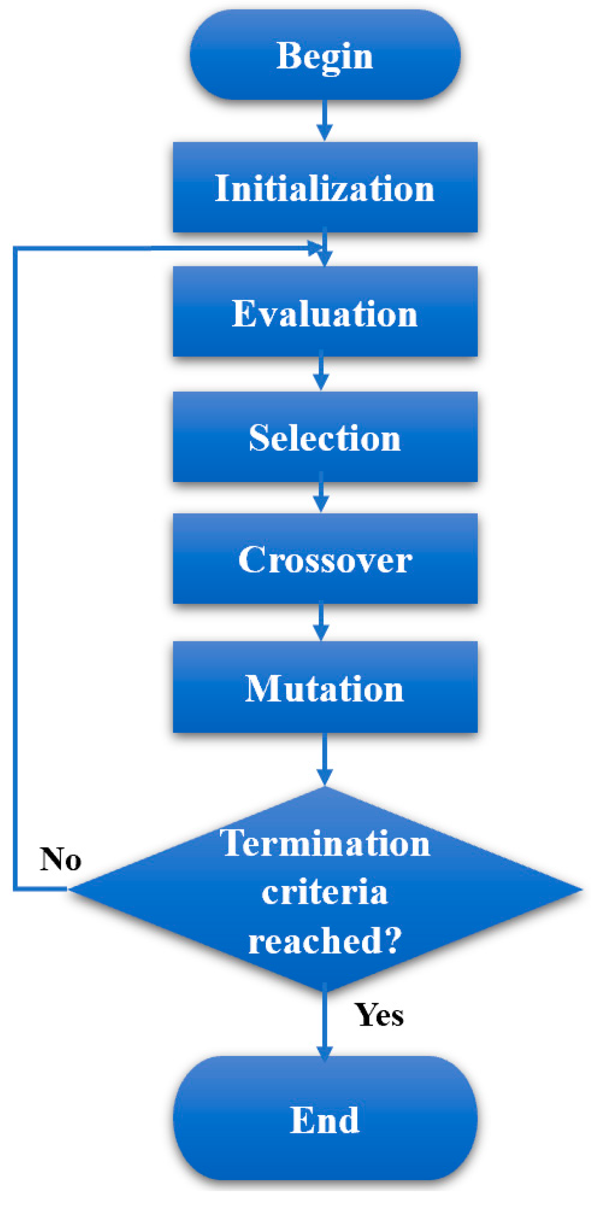
• Additionally, multi-objective optimization of process parameters using different weighting methods and the genetic algorithm (GA) was conducted for precision face milling of maraging steel 350.

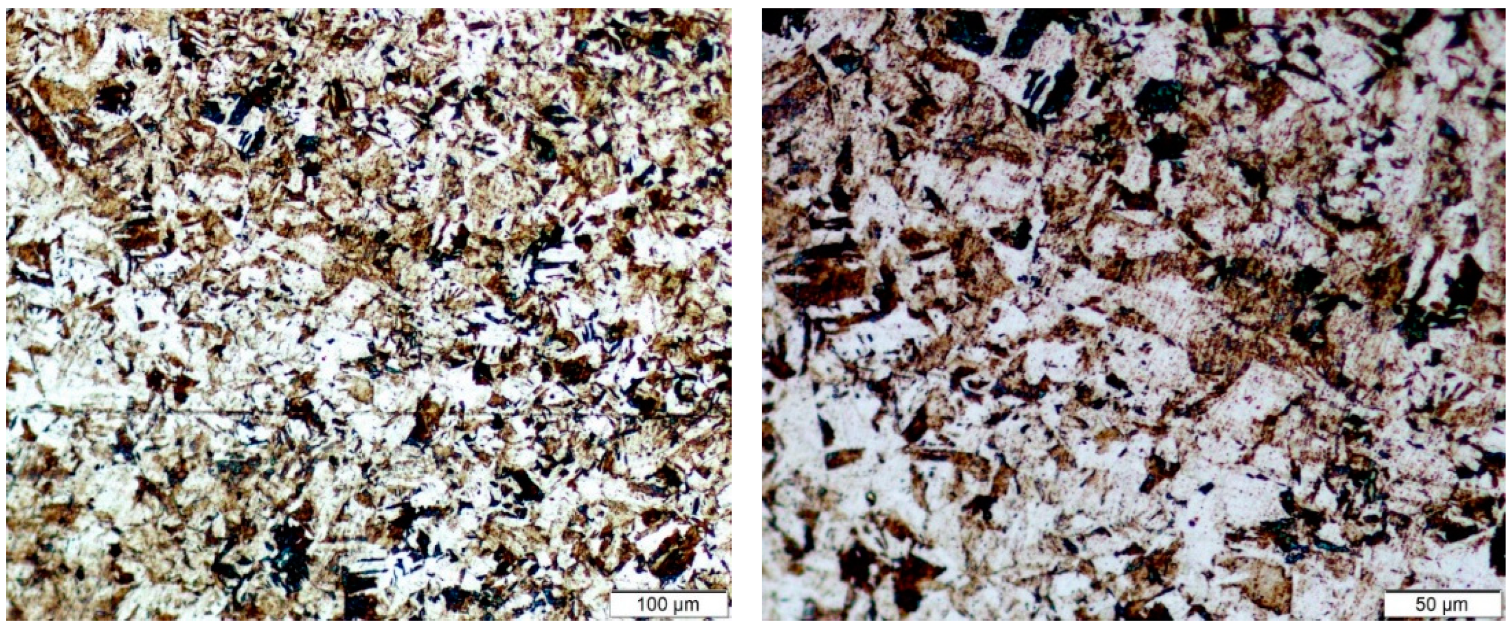
2. Materials Preparation and Methodology

The workpiece utilized in this research was maraging steel 350 delivered in a hot-rolled and air-cooled plate of 32 mm in thickness. The chemical composition listed in

Table 1. Chemical composition of maraging steel 350.

Element	Ni	Co	Mo	Ti	Al	Cu	C	Cr	Mn	Fe
weight (wt.%)	18.164	12.173	4.06	2.211	0.147	0.010	0.032	0.004	0.022	63.177

was analyzed using a Spectro graphical analysis-type SPECTROMAXx-LMM05, manufactured by AMETEK, Inc. (Berwyn, PA, USA), while

Table 2. Mechanical properties.

Description	Unit	Value
Ultimate tensile strength	MPa	1132
Yield strength	MPa	1080
Young’s modulus	GPa	200
Elongation	%	22.5
Hardness	HRc	38

lists the mechanical properties that were ascertained through a tensile specimen test with L_o =34 mm and d_o = 6.2 mm, using an INSTRON-5984 Universal Testing Machine manufactured by Instron Corporation (Norfolk County, MA, USA).

The specimen was grinded with various grades of sandpapers, including 120, 180, 500, and 1000, and then was polished with SiC and alumina cloth polishers. Afterward, the samples were etched in V2A solution (HCl 119 mL, HNO3 12 mL, and distilled water 119 mL). Microstructural analysis was conducted using an Olympus BX51RF optical microscope (Tokyo-Japan), as shown in Figure 1. The microstructure consisted of fine morphology with martensite packets within prior austenite grains. The martensite was soft because of its low carbon content. These steels’ high strength and hardness are procured after aging in the temperature range of 500–600 °C due to the precipitation of fine particles of Ni3(Mo, Ti) intermetallic compounds in the structure.

The experimental runs were conducted using workpieces with dimensions of 100 mm, 50 mm, and 30 mm for the length, width, and height, respectively. An Emco vertical milling machine type C40 was utilized for the face milling of maraging steel. The power delivered to the spindle was 13 KW, rotating in the range of 10–5000 RPM, while the feed rate ranged from 10 to 2000 mm/min. The cutter and inserts were manufactured by Sandvik (Sandvik, Stockholm, Sweden). The holder was a milling cutter with code R245-063Q22-12M. In contrast, the insert code was R245-12T3M-PM 1130 with a cutting-edge effective length of 10 mm, depth of cut maximum of 6.5 mm, corner radius of 1.5 mm, insert rake angle of 15°; major cutting-edge angle of 45°, and a coating PVD AlTiCrN. The experimental runs were conducted using five inserts pinned in a 63-mm cutter diameter. The endmill is designed for high-quality surface quality and potent chip removal and is generally used for cutting several steel and titanium alloys. Figure 2 shows a schematic diagram of the experimental setup.

A factorial design was conducted using three factors at three various levels (L27). The variables included cutting speed, depth of cut (D.o.C), and feed per tooth. The levels of such variables were selected based on pilot tests in various conditions.

Table 3. Process parameters and levels.

Parameters	Unit	Levels
Cutting Speed	m/min	20	50	75
D.o.C	mm	0.5	0.75	1.0
Feed per Tooth	mm/tooth	0.05	0.10	0.15

lists the process parameters with their levels. All experimental runs were conducted in dry conditions with two replications, and the average value was used for statistical analysis.

The surface roughness parameters R_a, R_t, and R_z were measured using Tesa-Rougossurf-90G (Tesa company, Bugnon, Switzerland), with a cut-off length of 0.8 mm, a measurement speed of 1 mm/s, and a cut-off number of 19. The power consumption during face milling was assessed by two power meters (Tactix, Beijing, China) connected to the power supply of the milling machine to measure the voltage and current during machining. Consumed power was assessed by measurement of the current (I) in one line and the voltage difference (V) through a balanced three-phase load-cutting machine. Three readings were recorded for each experimental trial, and the average was evaluated. Therefore, the power (P) was calculated using Equation (1), where (ø) represents the power factor for a three-phase machine:

Total power = Voltage * Current * √3 COS ø = Watt

(1)

A ThermoPro-TP8 thermal camera from the Guide company (Wuhan, China) was used to capture the cutting temperature during experimental runs, and its specifications are listed in

Table 4. Thermal camera specifications.

Feature	Specification
Measurement Range	−20 to 1000 °C
Thermal Sensitivity	≤0.08 °C at 30 °C
Set Emissivity for Steel	0.18
Accuracy	±2 °C
Spectral Range	8–14 μm
Detector type	Micro-bolometer—UFPA384 × 288 pixels

. The camera was calibrated before experimental work by adjusting the focus of the camera. In turn, suitable sensitivity was adopted, and the camera focused on the interface between the workpiece and the milling cutter to accurately capture the maximum cutting temperature. Figure 3 shows the thermal image of experiment 16, while the material emissivity coefficient was selected based on the camera manufacturer’s recommendations.

3. Result and Discussion

This study’s outcomes are surface roughness, power consumption, cutting temperature, and material removal rate. Surface roughness was evaluated in terms of arithmetic mean roughness (Ra), total roughness (Rt), and mean depth of profile (Rz).

Table 5. Experimental runs and responses.

Test No.	Speed m/min	D.o.C (mm)	Feed Rate (mm/tooth)	Surface Roughness			Power Consumption (KW)	Temp. (°C)	MRR (mm3/min)
				Ra (µm)	Rt (µm)	Rz (µm)
1	25	0.5	0.05	0.753	8.606	4.92	1.147	234.2	800
2	25	0.5	0.1	0.765	8.729	5.489	1.2	241.9	1575
3	25	0.5	0.15	0.884	9.059	5.632	1.254	253.9	2375
4	25	0.75	0.05	0.601	7.236	3.79	1.207	265.5	1200
5	25	0.75	0.1	0.628	7.972	4.437	1.267	274.1	2363
6	25	0.75	0.15	0.691	8.286	4.688	1.307	287.8	3563
7	25	1	0.05	0.517	5.922	3.55	1.24	312.3	1600
8	25	1	0.1	0.543	6.972	4.029	1.3	322.5	3150
9	25	1	0.15	0.585	7.324	4.335	1.32	338.6	4750
10	50	0.5	0.05	0.261	3.905	1.768	1.347	328.7	1575
11	50	0.5	0.1	0.52	7.081	3.334	1.414	339.5	3150
12	50	0.5	0.15	0.674	9.124	4.427	1.467	356.4	4750
13	50	0.75	0.05	0.256	3.259	1.724	1.414	372.6	2363
14	50	0.75	0.1	0.634	4.489	3.248	1.487	384.7	4725
15	50	0.75	0.15	0.813	12.477	4.071	1.52	403.9	7125
16	50	1	0.05	0.371	3.494	2.296	1.48	438.3	3150
17	50	1	0.1	0.592	5.201	3.231	1.534	452.6	6300
18	50	1	0.15	0.698	6.73	3.993	1.567	475.2	9500
19	75	0.5	0.05	0.365	5.164	2.057	1.42	427.3	2375
20	75	0.5	0.1	0.606	4.965	3.686	1.54	441.4	4750
21	75	0.5	0.15	0.652	3.682	3.299	1.614	463.3	7100
22	75	0.75	0.05	0.842	5.361	4.747	1.567	484.4	3563
23	75	0.75	0.1	0.858	6.363	5.479	1.654	500.1	7125
24	75	0.75	0.15	0.875	7.042	5.983	1.68	525.1	10,650
25	75	1	0.05	0.886	7.763	3.592	1.607	569.8	4750
26	75	1	0.1	0.902	8.307	4.307	1.76	588.4	9500
27	75	1	0.15	0.989	8.695	4.835	1.88	617.8	14,200

displays the experimental runs along with their corresponding responses.

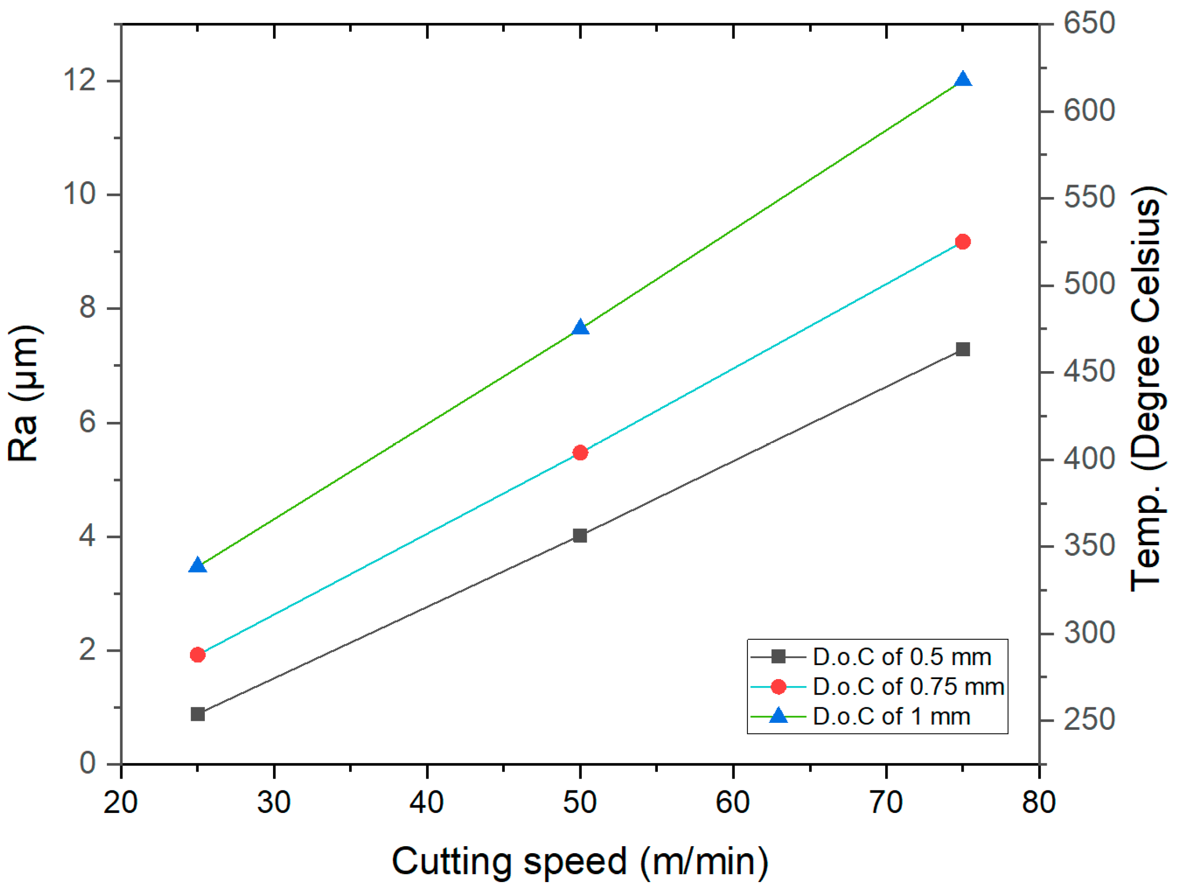
3.1. Effect of Process Parameters on Surface Quality

The ANOVA presented in

Table 6. Analysis of variance of Ra.

Source	DF	Adj SS	Adj MS	F-Value	p-Value
Speed	2	0.259	0.129	34.940	0.000	Significant
D.o.C	2	0.033	0.017	4.470	0.050	Not Significant
Feed rate	2	0.227	0.113	30.660	0.000	Significant
Speed * D.o.C	4	0.330	0.082	22.280	0.000	Significant
Speed * Feed rate	4	0.109	0.027	7.370	0.009	Significant
D.o.C * Feed rate	4	0.010	0.003	0.680	0.623	Not Significant
Error	8	0.030	0.004
Total	26	0.997

reveals that cutting speed was the most influential parameter affecting Ra, followed by feed rate. An increase in cutting speed resulted in smaller chip thickness, which improved surface quality by reducing roughness. Consequently, the interaction between cutting speed and D.o.C and the interaction between speed and feed rate significantly affected the Ra. However, elevating the cutting speed beyond 50 m/min adversely impacted surface quality, as depicted in Figure 4. This phenomenon occurred because a 75 m/min cutting speed amplifies the heat generated by excessive friction between the cutting tool and the workpiece. The resultant rise in cutting temperature compromises surface quality. Consequently, a 50 m/min cutting speed emerged as a threshold beyond which the surface finish deteriorated.

Additionally, augmenting the feed rate increased chip thickness, detracting from the smoothness of the machined surface and yielding higher surface roughness. Conversely, the depth of cut exerted a less pronounced impact on Ra. This outcome can be attributed to the efficient trimming of the chip thickness facilitated by overlapping the five inserts. Therefore, the interaction of D.o.C and feed rate did not significantly affect the Ra. Generally, a reduced depth of cut yielded a finer chip thickness, improving the machined surface quality, as illustrated in Figure 4.

A similar pattern was observed for Rt and Rz, indicating that increased D.o.C and feed rate led to elevated surface roughness. Figure 5 compares the Ra, Rt, and Rz values at a 75 m/min cutting speed across various feed rates and D.o.C levels. Regarding Rt and Rz, the interaction between minimal D.o.C and increased feed rate reduced the maximum lengths of the peaks and valleys in the surface roughness profile, leading to lower Rt and Rz values. However, this interaction was not observed for Ra, as Ra represents the arithmetic mean roughness along the entire cutting length of the workpiece. Additionally, regression equations were developed to predict Ra, Rt, and Rz values, as represented in Equations (2), (3), and (4), respectively:

Ra = 1.056 − 0.01776 Speed − 0.918 D.o.C + 3.45 Feed rate + 0.02548 Speed * D.o.C + 0.0089 Speed * Feed rate − 2.22 D.o.C * Feed rate

(2)

Rt = 14.44 − 0.1878 Speed − 12.32 D.o.C + 23.1 Feed rate + 0.2284 Speed * D.o.C − 0.118 Speed * Feed rate + 9.2 D.o.C * Feed rate

(3)

Rz = 6.84 − 0.0934 Speed − 4.72 D.o.C + 14.3 Feed rate + 0.1043 Speed * D.o.C + 0.088 Speed * Feed rate − 5.9 D.o.C * Feed rate

(4)

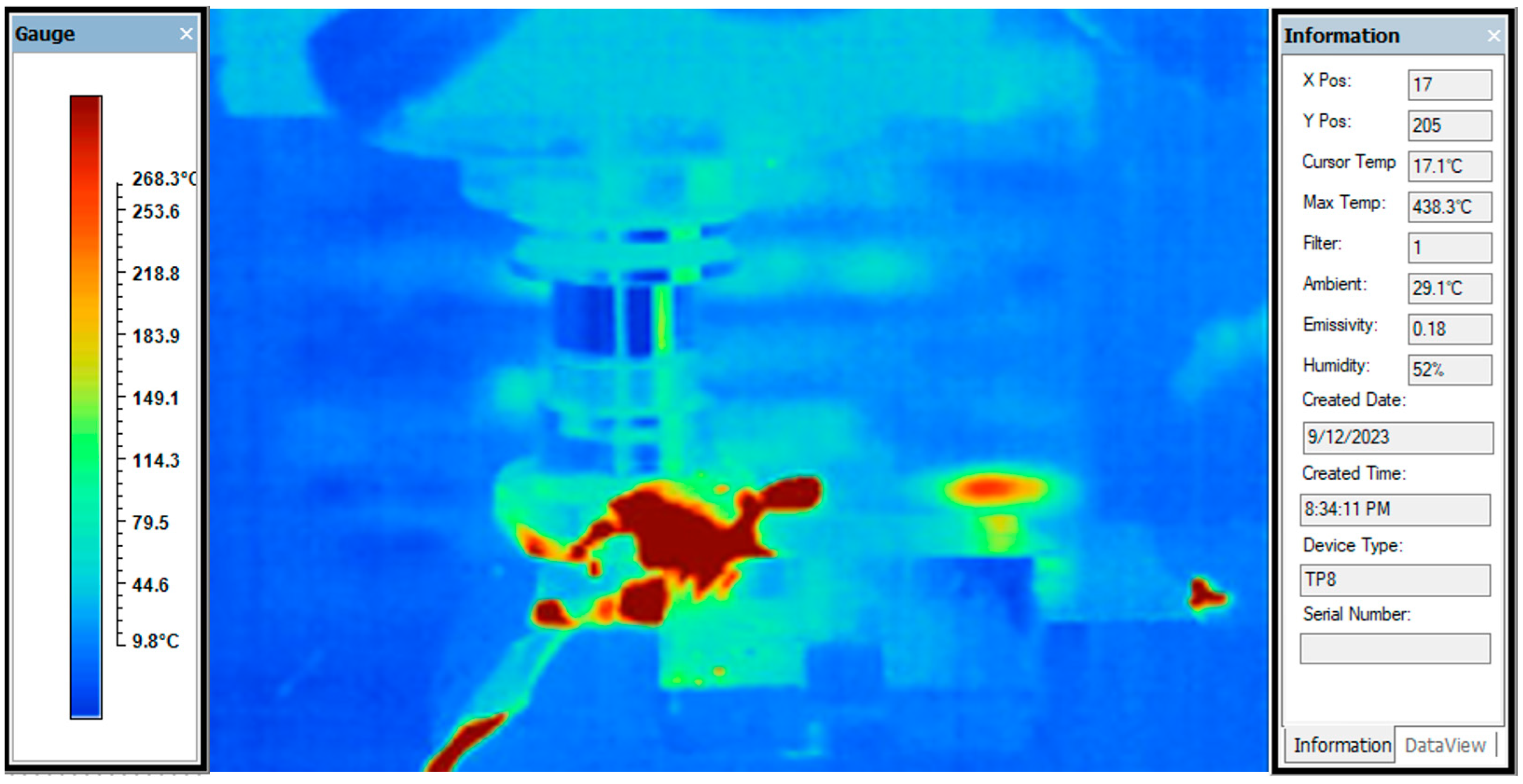
3.2. Effect of Process Parameters on Cutting Temperature

Monitoring the cutting temperature is crucial in machining operations because it not only affects the strength of the workpiece but also impacts chip removal efficiency. Elevated cutting temperatures can lead to rapid tool wear, subsequently deteriorating surface quality. As illustrated in Figure 6, the cutting temperature increased dramatically with increased cutting speed, leading to compromised surface quality.

Furthermore, the analysis of variance displayed in

Table 7. Analysis of variance of cutting temperature.

Source	DF	Adj SS	Adj MS	F-Value	p-Value
Speed	2	241,967	120,983	255,398.59	0.000	Significant
D.o.C	2	59,597	29,798	62,904.97	0.000	Significant
Feed rate	2	4714	2357	4976.07	0.000	Significant
Speed * D.o.C	4	3399	850	1793.74	0.000	Significant
Speed * Feed rate	4	270	67	142.25	0.000	Significant
D.o.C * Feed rate	4	67	17	35.20	0.000	Significant
Error	8	4	0
Total	26	310,016

underscored that all process parameters and their interactions significantly impacted the cutting temperature. Among these parameters, cutting speed stands out as the most influential due to the excessive friction generated between the workpiece and the five inserts. A direct correlation among cutting temperature, the number of inserts, and flank wear was articulated by Richetti et al. [30]. In light of these findings, the primary objective of this study was to optimize the process parameters to attain lower cutting temperatures and surface roughness values. These aspects are elaborated upon in the subsequent sections. A regression equation, represented by Equation (5), was also formulated to predict cutting temperature:

Temp. = 93.9 + 2.255 Speed + 76.4 D.o.C − 6 Feed rate + 2.675 Speed * D.o.C + 3.76 Speed * Feed rate + 185 D.o.C * Feed rate

(5)

3.3. Effect of Process Parameters on MRR and Power Consumption

While a high material removal rate benefits mass production and economic growth, excessive power consumption poses a significant environmental concern. Consequently, comprehensively understanding and optimizing process parameters is essential to strike a balanced compromise between these conflicting responses. As depicted in

Table 8. Analysis of Variance of power consumption.

Source	DF	Adj SS	Adj MS	F-Value	p-Value
Speed	2	0.677	0.339	482.270	0.000	Significant
D.o.C	2	0.092	0.046	65.490	0.000	Significant
Feed rate	2	0.079	0.039	56.070	0.000	Significant
Speed * D.o.C	4	0.016	0.004	5.730	0.018	Significant
Speed * Feed rate	4	0.009	0.002	3.190	0.076	Not Significant
D.o.C * Feed rate	4	0.002	0.000	0.540	0.711	Not Significant
Error	8	0.006	0.001
Total	26	0.880

, ANOVA highlighted that all process parameters markedly influence power consumption. Cutting speed emerges as the paramount factor, primarily because a rise in speed amplifies the friction between the tool and workpiece. This intensification in friction precipitates a dramatic escalation in insert wear and cutting forces. In a similar vein, elevating the D.o.C and feed rate augments power consumption, a trend clearly illustrated in Figure 7a. This increase can be imputed to the amplified cutting forces resulting from enhanced chip thickness.

Moreover, the material removal rate (MRR) surges significantly with the escalation in both the depth of cut and the feed rate, a phenomenon attributable to the increased chip thickness, as delineated in Figure 7b. Figure 8 presents a correlation plot mapping the relationships between machining parameters and responses. In this visual representation, dark blue signifies the most negative correlation (−1), whereas dark red indicates the peak positive correlation (+1). In this context, a positive correlation denotes that the specified response amplifies with an increase in machining parameters. In contrast, a negative correlation signifies that the chosen response diminishes as the machining parameters rise. To facilitate predictive analysis, regression equations for power consumption (PC) and MRR were formulated, as expressed in Equations (6) and (7), respectively:

PC = 1.0339 + 0.00164 Speed − 0.0031 D.o.C + 0.239 Feed rate + 0.00552 Speed * D.o.C + 0.01953 Speed * Feed rate + 0.127 D.o.C * Feed rate

(6)

MRR = 4725 − 94.5 Speed − 6311 D.o.C − 47,247 Feed rate + 126.3 Speed * D.o.C + 944.9 Speed * Feed rate + 63,167 D.o.C * Feed rate

(7)

4. ML Algorithms Adopted

The experimental data were utilized to train and test five distinct ML models aiming to predict machining parameters, encompassing SVM, KNN, ANN, random forest, and XGBoost. The SVM, a versatile method applied for classification and regression, operates by identifying a hyperplane that optimally separates different categories in n-dimensional space, ensuring that each is on the other side of the hyperplane. The SVM aims to maximize the margin, which is the distance to the nearest point from either category [31]. KNN is another straightforward, supervised ML algorithm primarily used for classification. It classifies new data points based on the classification of their neighbors, with the number of neighbors considered during classification denoted by the parameter KN [31]. The human brain’s neural networks inspire ANNs and are adept at recognizing patterns within data. These data comprise input, hidden, and output layers of neurons, with the hidden layers performing the bulk of computations. Data are propagated through the network via forward propagation, involving weights, biases, and activation functions [32]. Random forest amalgamates the strengths of bagging and decision trees, reducing sensitivity to training data. It builds multiple decision trees using bootstrapped datasets, and their results are aggregated to enhance the model’s robustness and accuracy. Each tree in the forest is trained on a variant dataset, ensuring diversity and reducing correlation among the trees [33]. XGBoost, or extreme gradient boosting, combines the advantages of both bagging and boosting. It consists of a series of models in which each subsequent model corrects the errors of its predecessor, amplifying the overall predictive accuracy and model strength [34].

5. Comparative Results of ML Algorithms

The five ML approaches were employed to discern the correlation between input parameters and various performance characteristics, including surface roughness, power consumption, cutting temperature, and MRR. Twenty-six experimental results, as outlined in Table 3, were utilized for training, with one remaining dataset reserved for testing the predictive efficacy of the five models. The comparative analysis of each ML model’s accuracy is presented in

Table 9. Testing five ML models.

		Ra (µm)	Rt (µm)	Rz (µm)	PC (KW)	Temp. (°C)	MRR (mm3/min)
	Actual	0.902	8.307	4.307	1.76	588.4	9500
KNN	Predicted	0.79	6.50	4.08	1.63	505.00	7420.00
	Percentage Correctness	0.877827	0.782737	0.946599	0.9275	0.85826	0.781053
XGBOOST	Predicted	0.87	8.28	4.18	1.81	596.44	9688.08
	Percentage Correctness	0.960451	0.996439	0.970013	0.968806	0.986336	0.980203
ANN	Predicted	0.94	5.14	4.16	1.58	13.28	13.23
	Percentage Correctness	0.952647	0.618528	0.966594	0.895583	0.022562	0.001393
SVR	Predicted	0.85	6.76	4.30	1.66	382.43	3565.77
	Percentage Correctness	0.940451	0.814061	0.997267	0.941342	0.649956	0.375344
Random Forest	Predicted	0.83	6.88	4.36	1.70	572.75	7207.50
	Percentage Correctness	0.922517	0.828719	0.98671	0.963687	0.973408	0.758684

.

The hyperparameters for the machine learning models used in the analysis were five neighbors, and the Euclidean distance metric was employed for the KNN model. In the case of XGBoost, a popular gradient boosting algorithm, a configuration with 100 trees, a maximum tree depth of 3, and a learning rate of 0.3 was used. The ANN model utilized a single hidden layer with 100 neurons and the Rectified linear unit (ReLU) activation function. The support vector regressor (SVR) had a radial Basis function (RBF) kernel, with the regularization parameter (C) as 1.0 and an epsilon value of 0.1. Last, we maintained settings with 100 trees and unlimited tree depth for the random forest regressor.

It was observed that the XGBoost model delivered predictions closely aligned with the actual values for all performance characteristics, outperforming the other ML models. This superior performance can be attributed to XGBoost’s ensemble learning nature, according to which it combines predictions from multiple machine learning algorithms to generate a final prediction that is more accurate and stable. It also incorporates regularization techniques, such as L1 and L2 regularization, effectively reducing the model’s complexity and preventing overfitting. As a result, the XGBoost model demonstrates enhanced adaptability, making precise predictions even when introduced to new, unseen data.

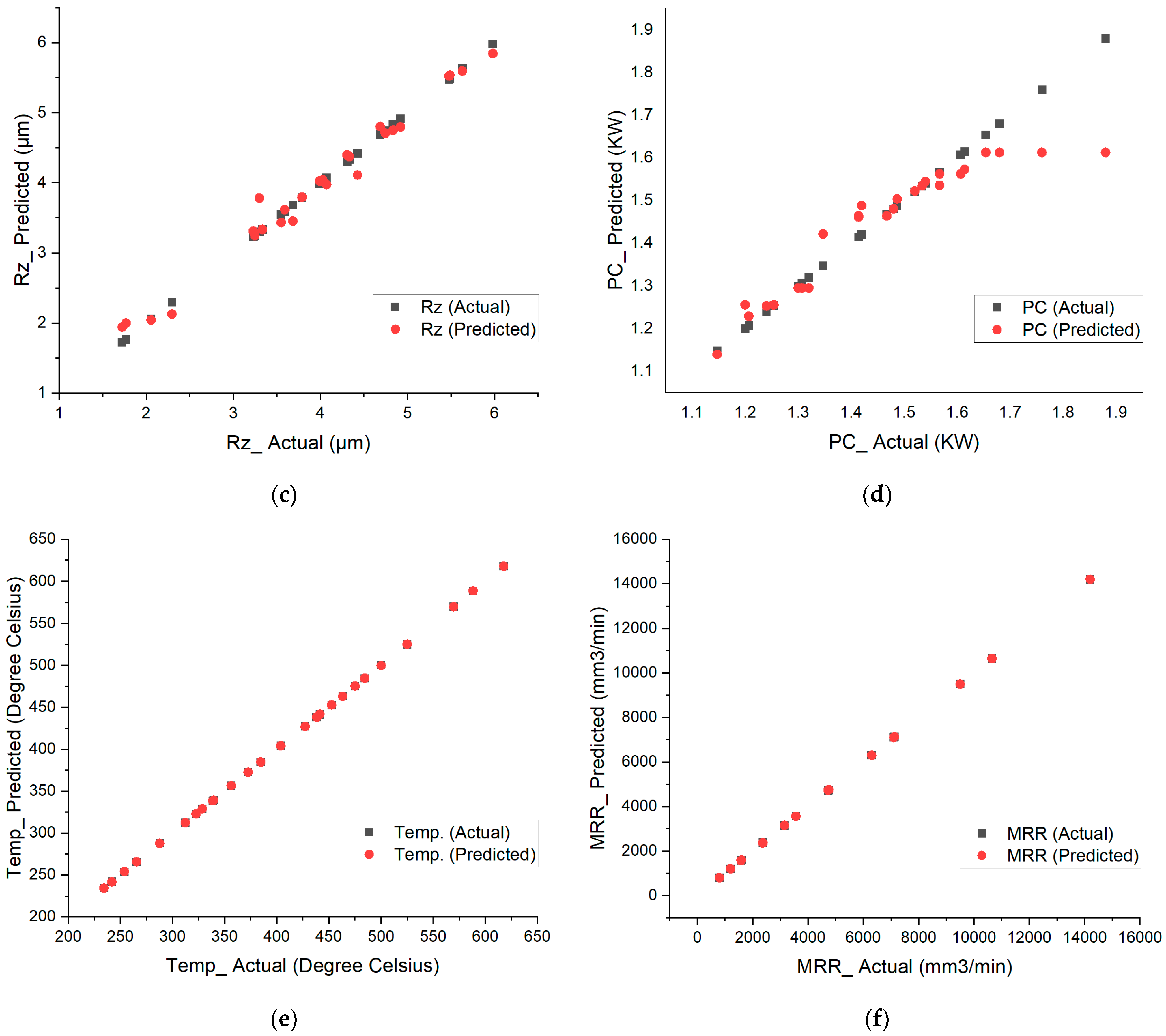
6. Optimal XGBoost Prediction of Responses

Typically, hyperparameters are determined through a trial-and-error process. However, this method does not always ensure optimal performance. This study employs a genetic algorithm (GA) to optimize the XGBoost hyperparameters. The GA is an evolutionary algorithm inspired by natural selection and genetic theories. It involves selecting chromosomes from a population based on their fitness values. This process is followed by a crossover process, combining two chromosomes to create a new one. Subsequently, a mutation occurs, involving a random alteration of some bits in the chromosome. This outcome introduces diversity into the population and helps to avoid local optima, ensuring a more comprehensive search for global optimal solutions, as illustrated in Figure 9. The objective is to select the best chromosomes to form the next generation [35].

Table 10. Optimal hyperparameters.

Hyperparameter Parameter	Optimal Value
Maximum Depth	4
Number of Estimators	365
Subsample	0.247020091
Colsample by Tree	0.829416734
Regularization Alpha	0.188535466
Regularization Lambda	0.980953654

presents the optimal values of the hyperparameters for XGBoost obtained through GA. These optimal hyperparameters were employed to predict the performance characteristics for all experimental runs, the results of which are detailed in

Table 11. Optimal XGBoost Model results.

	Predicted						Actual
Order	Ra (µm)	Rt (µm)	Rz (µm)	PC (KW)	Temp. (°C)	MRR (mm3/min)	Ra (µm)	Rt (µm)	Rz (µm)	PC (KW)	Temp. (°C)	MRR (mm3/min)
3	0.6948	8.9826	5.5978	1.2552	254.1231	2374.803	0.884	9.059	5.632	1.254	253.9	2375
1	0.5875	8.4114	4.7987	1.1394	234.2131	799.9993	0.753	8.606	4.92	1.147	234.2	800
4	0.5875	7.2322	3.7959	1.2288	265.4778	1199.994	0.601	7.236	3.79	1.207	265.5	1200
8	0.6001	6.8984	4.0436	1.2949	322.7358	3149.850	0.543	6.972	4.029	1.3	322.5	3150
23	0.8302	6.2875	5.5252	1.6128	499.8404	7125.210	0.858	6.363	5.479	1.654	500.1	7125
6	0.6948	8.3705	4.8029	1.2949	287.6072	3563.305	0.691	8.286	4.688	1.307	287.8	3563
18	0.657	6.8045	4.0277	1.5357	475.1958	9500.082	0.698	6.73	3.993	1.567	475.2	9500
19	0.4843	4.9828	2.0431	1.4883	427.1518	2375.214	0.365	5.164	2.057	1.42	427.3	2375
26	0.8302	8.2402	4.3994	1.6128	588.4298	9500.226	0.902	8.307	4.307	1.76	588.4	9500
2	0.6684	8.8814	5.5383	1.2552	241.824	1575.122	0.765	8.729	5.489	1.2	241.9	1575
27	0.8566	8.6883	4.7501	1.6128	617.7504	14,199.80	0.989	8.695	4.835	1.88	617.8	14,200
10	0.4643	4.2384	2.0001	1.4217	328.8993	1574.773	0.261	3.905	1.768	1.347	328.7	1575
22	0.7671	5.3605	4.7104	1.5624	484.7287	3562.817	0.842	5.361	4.747	1.567	484.4	3563
11	0.6001	6.9588	3.3356	1.464	339.1916	3150.316	0.52	7.081	3.334	1.414	339.5	3150
15	0.657	12.0827	3.9767	1.5223	404.0421	7124.864	0.813	12.477	4.071	1.52	403.9	7125
21	0.6945	4.0596	3.7828	1.5731	462.9821	7100.231	0.652	3.682	3.299	1.614	463.3	7100
9	0.6507	7.325	4.3751	1.2949	338.3776	4750.052	0.585	7.324	4.335	1.32	338.6	4750
14	0.6065	4.687	3.2458	1.5037	384.6817	4724.958	0.634	4.489	3.248	1.487	384.7	4725
13	0.4643	3.3416	1.9411	1.4614	372.3993	2363.066	0.256	3.259	1.724	1.414	372.6	2363
24	0.8566	7.1392	5.8478	1.6128	525.2257	10,649.85	0.875	7.042	5.983	1.68	525.1	10,650
17	0.6065	5.2128	3.3118	1.5347	452.7394	6299.734	0.592	5.201	3.231	1.534	452.6	6300
20	0.618	4.9388	3.4556	1.5448	441.6176	4749.693	0.606	4.965	3.686	1.54	441.4	4750
12	0.6507	8.9212	4.1137	1.464	356.6009	4749.916	0.674	9.124	4.427	1.467	356.4	4750
16	0.4707	3.5253	2.1291	1.4802	438.2168	3150.195	0.371	3.494	2.296	1.48	438.3	3150
25	0.7671	7.7504	3.6168	1.5624	569.7158	4749.959	0.886	7.763	3.592	1.607	569.8	4750
7	0.5207	5.9012	3.4344	1.2526	312.2711	1599.980	0.517	5.922	3.55	1.24	312.3	1600

.

Figure 10 displays a scatter plot comparing the actual dataset with the results predicted by the optimized XGBoost model. It is observable that the predicted responses for Rt, Rz, cutting temperature, and MRR align closely with the actual values. While there is a slight deviation in the predicted Ra and recorded power consumption, the error margin remains minimal, at 1.4% for Ra and 0.9% for power consumption. These small error margins underscore the reliability of the optimized XGBoost model in accurately modeling and predicting the machining parameters.

7. Multi-Objective Optimization of Process Parameters

GA was employed for the multi-objective optimization of process parameters, aiming to minimize responses, including arithmetic mean roughness (Ra), cutting temperature, and power consumption. The assignment of importance weights to these responses is a crucial step in the optimization process. While many researchers have defaulted to assigning equal weights to each response, an alternative approach involves customizing these weights based on industrial requirements or insights gathered from expert surveys. In this study, we explored both methods: equal weight assignment and the analytic hierarchy process (AHP).

The AHP facilitates the calculation of weights for each response, grounded in data sourced from expert surveys. This methodology is instrumental in discerning the relative significance of diverse attributes in relation to overarching objectives.

Table 12. Saaty’s nine-point scale of relative importance.

Scale	Definition	Explanation
1	Equally Important	Indifferent
3	Weakly Important	Slightly better
5	Strongly Important	Better
7	Very Strongly Important	Much better
9	Extremely Important	Definitely much better
2, 4, 6, 8	Intermediate value	When compromise needed

presents Saaty’s nine-point preference scale, which serves as the foundation for constructing a pairwise comparison matrix [36].

Equation (8) is used to construct a pairwise comparison matrix (B_mxm), where (B_m) represents the criteria, and m denotes the number of criteria. Each criterion (B_i) is compared pairwise with every other criterion (B_j). Based on surveys conducted, the relative importance is assigned to each row criterion (B₁, B₂, …, B_m) by comparing it with each column criterion (B₁, B₂, …, B_m), as detailed in

Table 13. Pairwise comparison matrix.

Criteria	Ra	PC	Temp.	MRR
Ra	1	9	5	5
PC	1/9	1	1/7	1/5
Temp.	1/5	7	1	3
MRR	1/5	5	1/3	1

.

$$B_{\mathrm{m}\mathrm{x}\mathrm{m}}=\left[\begin{array}{cc}\begin{array}{cc}1& b_{12}\\ b_{21}& 1\end{array}& \begin{array}{cc}{--b}_{1j}& {--b}_{1m}\\ {--b}_{2j}& {--b}_{2m}\end{array}\\ \begin{array}{cc}{b}_{i1}& b_{i2}\\ b_{m1}& b_{m2}\end{array}& \begin{array}{cc}--b_{ij}& {--b}_{im}\\ {--b}_{mj}& --1\end{array}\end{array}\right]$$

(8)

The relative normalized weight (W_j) of each criterion is calculated using the ratio of the geometric mean (GMi) of the corresponding row in the pairwise comparison matrix (B_mxm) to the sum of the geometric means of all rows. This calculation is represented in Equations (9) and (10):

$${GM}_i={\left[{\prod }_{j=1}^m{b}_{ij}\right]}^{\frac{1}{m}}$$

(9)

$$w_j={GM}_i/{\sum }_{i=1}^m{GM}_i$$

(10)

Equation (11) is employed to compute the consistency index (CI), with λ_max representing the maximum eigenvalue of the matrix. λ_max is derived by averaging the sum of the matrix product of the pairwise comparison matrix and weight vectors and then dividing by the relative normalized weight of the corresponding attribute. A lower CI value indicates minimal deviation from consistency. The consistency ratio (CR) is calculated using Equation (12), with RI representing the random index value detailed in

Table 14. Random index (RI)/random judgment values [37].

No. of Criteria	1	2	3	4	5	6	7	8	9	19
RI	0.0	0.0	0.58	0.90	1.12	1.24	1.32	1.41	1.45	1.49

. Generally, a CR value of 0.10 or less indicates acceptable consistency:

$$CI=\frac{{\mathsf{\lambda }}_{max}-m}{m-1}$$

(11)

$$CR=\frac{CI}{RI}$$

(12)

Table 15. Equal weights compared to AHP weights.

Criteria	AHP Weights	Equal Weights
Ra	0.510369	0.25
Power Consumption	0.037103	0.25
Temp	0.285807	0.25
MRR	0.166721	0.25

enumerates the weights assigned to each response using both methods. These weights were applied in the multi-objective optimization utilizing a genetic algorithm (GA), with the optimized parameters detailed in

Table 16. Optimal input parameters with their predicted responses.

	Optimal Input			Output
Weighting Methods	Speed m/min	D.o.C (mm)	Feed Rate (mm/tooth)	Ra (µm)	PC (KW)	Temp. (°C)	MRR (mm3/min)
Equal Weights	50	0.5	0.05	2.54	1.42	328.97	1608.83
AHP Weights	50	0.5	0.15	2.58	1.35	319.92	1613.64

. A close examination reveals that the output responses for each weighting method are nearly identical, suggesting that the model is closely approaching the global optima.

8. Conclusions

This study of the machining of maraging steel—a material distinguished for its outstanding strength-to-weight ratio—produced results that connect experimental observations with predictive modeling. The experiments revealed intricate relationships between face milling parameters and critical performance indicators, including surface roughness, cutting temperature, power consumption, and MRR. From this study, the following specific insights emerged:

• The intricate interplay between cutting speed and feed rate has been identified as a pivotal factor influencing surface finish. A 50 m/min cutting speed threshold was recognized, beyond which surface roughness escalated due to heightened friction and temperature;
• Increasing the cutting speed led to a proportional rise in cutting temperature. These insights underline the need for strategic control of speed to mitigate thermal effects, optimizing tool longevity and surface integrity;
• The relationship between power consumption and MRR in terms of cutting speed, D.o.C, and feed rate was established. This relationship provides a foundational understanding for balancing operational efficiency with energy consumption;
• Among the evaluated machine learning models, XGBoost demonstrated superior performance, validating its aptitude for modeling complex, non-linear relationships inherent in machining processes. Its predictive accuracy stood at a commendable 98%;
• The employment of the genetic algorithm (GA) in optimizing XGBoost’s hyperparameters further refined the model’s predictive power. The optimization balanced multiple objectives, ensuring holistic performance improvement;
• A comparative analysis of equal weights and AHP-based weights emphasized the consistency in optimization outcomes, underscoring the model’s robustness and adaptability to diverse weighting scenarios.

One can finally conclude that the confluence of experimental analyses and different machine learning models has opened avenues for enhanced machining precision, efficiency, and sustainability in dealing with maraging steel. The insights gained are not only instrumental in understanding the inherent machining challenges but are also pivotal in navigating them, promising enhanced operational efficiency and product quality. As industries strive for heightened efficiency, reduced operational costs, and sustainable practices, the results of this study serve as a step forward, illuminating pathways for informed decision-making and strategic interventions in the face milling of maraging steel. Future research could explore the scalability of these findings across diverse steel grades and machining contexts, amplifying the impacts of these insights on industrial applications globally.

References

1. Pardal, J.; Tavares, S.; Terra, V.; Da Silva, M.; Dos Santos, D. Modeling of precipitation hardening during the aging and overaging of 18Ni–Co–Mo–Ti maraging 300 steel. J. Alloys Compd. 2005, 393, 109–113. [Google Scholar] [CrossRef]
2. Chandraker, S. Taguchi analysis on cutting force and surface roughness in turning MDN350 steel. Mater. Today Proc. 2015, 2, 3388–3393. [Google Scholar]
3. Jägle, E.A.; Choi, P.-P.; Van Humbeeck, J.; Raabe, D. Precipitation and austenite reversion behavior of a maraging steel produced by selective laser melting. J. Mater. Res. 2014, 29, 2072–2079. [Google Scholar] [CrossRef]
4. Casalino, G.; Campanelli, S.; Contuzzi, N.; Ludovico, A. Experimental investigation and statistical optimisation of the selective laser melting process of a maraging steel. Opt. Laser Technol. 2015, 65, 151–158. [Google Scholar] [CrossRef]
5. Fortunato, A.; Lulaj, A.; Melkote, S.; Liverani, E.; Ascari, A.; Umbrello, D. Milling of maraging steel components produced by selective laser melting. Int. J. Adv. Manuf. Technol. 2018, 94, 1895–1902. [Google Scholar] [CrossRef]
6. Santhanakumar, M.; Adalarasan, R.; Siddharth, S.; Velayudham, A. An investigation on surface finish and flank wear in hard machining of solution treated and aged 18% Ni maraging steel. J. Braz. Soc. Mech. Sci. Eng. 2017, 39, 2071–2084. [Google Scholar] [CrossRef]
7. Stachurski, W.; Sawicki, J.; Wójcik, R.; Nadolny, K. Influence of application of hybrid MQL-CCA method of applying coolant during hob cutter sharpening on cutting blade surface condition. J. Clean. Prod. 2018, 171, 892–910. [Google Scholar] [CrossRef]
8. Benedicto, E.; Carou, D.; Rubio, E. Technical, economic and environmental review of the lubrication/cooling systems used in machining processes. Procedia Eng. 2017, 184, 99–116. [Google Scholar] [CrossRef]
9. Sharma, V.S.; Singh, G.; Sørby, K. A review on minimum quantity lubrication for machining processes. Mater. Manuf. Process. 2015, 30, 935–953. [Google Scholar] [CrossRef]
10. Tomaz, Í.V.; Pardal, J.M.; Fonseca, M.C. Influence of minimum quantity lubrication in the surface quality of milled maraging steel. Int. J. Adv. Manuf. Technol. 2019, 104, 4301–4311. [Google Scholar] [CrossRef]
11. Helmy, M.O.; El-Hofy, M.; El-Hofy, H. Effect of cutting fluid delivery method on ultrasonic assisted edge trimming of multidirectional CFRP composites at different machining conditions. Procedia CIRP 2018, 68, 450–455. [Google Scholar] [CrossRef]
12. Helmy, M.O.; El-Hofy, M.; El-Hofy, H. Influence of process parameters on the ultrasonic assisted edge trimming of aerospace CFRP laminates using MQL. Int. J. Mach. Mach. Mater. 2020, 22, 349–373. [Google Scholar] [CrossRef]
13. Beake, B.; Ning, L.; Gey, C.; Veldhuis, S.; Kornberg, A.; Weaver, A.; Khanna, M.; Fox-Rabinovich, G. Wear performance of different PVD coatings during hard wet end milling of H13 tool steel. Surf. Coat. Technol. 2015, 279, 118–125. [Google Scholar] [CrossRef]
14. Mo, J.; Zhu, M.; Leyland, A.; Matthews, A. Impact wear and abrasion resistance of CrN, AlCrN and AlTiN PVD coatings. Surf. Coat. Technol. 2013, 215, 170–177. [Google Scholar] [CrossRef]
15. Mo, J.; Zhu, M. Sliding tribological behaviors of PVD CrN and AlCrN coatings against Si3N4 ceramic and pure titanium. Wear 2009, 267, 874–881. [Google Scholar] [CrossRef]
16. Varghese, V.; Akhil, K.; Ramesh, M.; Chakradhar, D. Investigation on the performance of AlCrN and AlTiN coated cemented carbide inserts during end milling of maraging steel under dry, wet and cryogenic environments. J. Manuf. Process. 2019, 43, 136–144. [Google Scholar] [CrossRef]
17. Lou, S.; Jiang, X.; Sun, W.; Zeng, W.; Pagani, L.; Scott, P. Characterisation methods for powder bed fusion processed surface topography. Precis. Eng. 2019, 57, 1–15. [Google Scholar] [CrossRef]
18. Promoppatum, P.; Yao, S.-C. Analytical evaluation of defect generation for selective laser melting of metals. Int. J. Adv. Manuf. Technol. 2019, 103, 1185–1198. [Google Scholar] [CrossRef]
19. Bai, Y.; Yang, Y.; Xiao, Z.; Wang, D. Selective laser melting of maraging steel: Mechanical properties development and its application in mold. Rapid Prototyp. J. 2018, 24, 623–629. [Google Scholar] [CrossRef]
20. Mercelis, P.; Kruth, J.P. Residual stresses in selective laser sintering and selective laser melting. Rapid Prototyp. J. 2006, 12, 254–265. [Google Scholar] [CrossRef]
21. Withers, P.J.; Bhadeshia, H. Residual stress. Part 1–measurement techniques. Mater. Sci. Technol. 2001, 17, 355–365. [Google Scholar] [CrossRef]
22. Bhardwaj, T.; Shukla, M. Effect of laser scanning strategies on texture, physical and mechanical properties of laser sintered maraging steel. Mater. Sci. Eng. A 2018, 734, 102–109. [Google Scholar] [CrossRef]
23. Tamura, S.; Ezura, A.; Matsumura, T. Cutting Force in Peripheral Milling of Additively Manufactured Maraging Steel. Int. J. Autom. Technol. 2022, 16, 897–905. [Google Scholar] [CrossRef]
24. Oliveira, A.; Jardini, A.; Del Conte, E. Effects of cutting parameters on roughness and residual stress of maraging steel specimens produced by additive manufacturing. Int. J. Adv. Manuf. Technol. 2020, 111, 2449–2459. [Google Scholar] [CrossRef]
25. Abbas, A.T.; Sharma, N.; Alsuhaibani, Z.A.; Sharma, A.; Farooq, I.; Elkaseer, A. Multi-Objective Optimization of AISI P20 Mold Steel Machining in Dry Conditions Using Machine Learning—TOPSIS Approach. Machines 2023, 11, 748. [Google Scholar] [CrossRef]
26. Abbas, A.T.; Sharma, N.; Al-Bahkali, E.A.; Sharma, V.S.; Farooq, I.; Elkaseer, A. A Machine Learning Perspective to the Investigation of Surface Integrity of Al/SiC/Gr Composite on EDM. J. Manuf. Mater. Process. 2023, 7, 163. [Google Scholar] [CrossRef]
27. Chakraborty, D.; Elzarka, H. Advanced machine learning techniques for building performance simulation: A comparative analysis. J. Build. Perform. Simul. 2019, 12, 193–207. [Google Scholar] [CrossRef]
28. Abbas, A.T.; Pimenov, D.Y.; Erdakov, I.N.; Mikolajczyk, T.; Soliman, M.S.; El Rayes, M.M. Optimization of cutting conditions using artificial neural networks and the Edgeworth-Pareto method for CNC face-milling operations on high-strength grade-H steel. Int. J. Adv. Manuf. Technol. 2019, 105, 2151–2165. [Google Scholar] [CrossRef]
29. Zou, M.; Jiang, W.-G.; Qin, Q.-H.; Liu, Y.-C.; Li, M.-L. Optimized XGBoost model with small dataset for predicting relative density of Ti-6Al-4V parts manufactured by selective laser melting. Materials 2022, 15, 5298. [Google Scholar] [CrossRef]
30. Richetti, A.; Machado, A.; Da Silva, M.; Ezugwu, E.; Bonney, J. Influence of the number of inserts for tool life evaluation in face milling of steels. Int. J. Mach. Tools Manuf. 2004, 44, 695–700. [Google Scholar] [CrossRef]
31. Kilundu, B.; Dehombreux, P.; Chiementin, X. Tool wear monitoring by machine learning techniques and singular spectrum analysis. Mech. Syst. Signal Process. 2011, 25, 400–415. [Google Scholar] [CrossRef]
32. Han, T.; Jiang, D.; Zhao, Q.; Wang, L.; Yin, K. Comparison of random forest, artificial neural networks and support vector machine for intelligent diagnosis of rotating machinery. Trans. Inst. Meas. Control 2018, 40, 2681–2693. [Google Scholar] [CrossRef]
33. Prihatno, A.T.; Nurcahyanto, H.; Jang, Y.M. Predictive maintenance of relative humidity using random forest method. In Proceedings of the 2021 International Conference on Artificial Intelligence in Information and Communication (ICAIIC), Jeju Island, Republic of Korea, 13–16 April 2021; pp. 497–499. [Google Scholar]
34. Zhang, K.; Gu, C.; Zhu, Y.; Chen, S.; Dai, B.; Li, Y.; Shu, X. A novel seepage behavior prediction and lag process identification method for concrete dams using HGWO-XGBoost model. IEEE Access 2021, 9, 23311–23325. [Google Scholar] [CrossRef]
35. Lambora, A.; Gupta, K.; Chopra, K. Genetic algorithm—A literature review. In Proceedings of the 2019 International Conference on Machine Learning, Big Data, Cloud and Parallel Computing (COMITCon), Faridabad, India, 14–16 February 2019; pp. 380–384. [Google Scholar]
36. Nayak, B.; Mahapatra, S. Multi-response optimization of WEDM process parameters using the AHP and TOPSIS method. Int. J. Theor. Appl. Res. Mech. Eng. 2013, 2, 109–215. [Google Scholar]
37. Saaty, T.L. Decision making with the analytic hierarchy process. Int. J. Serv. Sci. 2008, 1, 83–98. [Google Scholar] [CrossRef]
Figure 1. Optical micrograph of maraging steel 350 with different magnifications.
Machines 11 01001 g001
Figure 2. Schematic diagram for face milling of maraging steel.
Machines 11 01001 g002
Figure 3. Thermal image for experiment 16 at which the cutting temp. is 438.3 °C.
Machines 11 01001 g003
Figure 4. Main effects plot for Ra.
Machines 11 01001 g004
Figure 5. Comparison among Ra, Rt, and Rz at different feed rates and D.o.C.
Machines 11 01001 g005
Figure 6. Correlation among cutting speed, Ra, and cutting temperature at various D.o.C.
Machines 11 01001 g006
Figure 7. (a) Main effect of power consumption (KW); (b) main effect for MRR (mm3/min).
Machines 11 01001 g007
Figure 8. Correlation plot between the machining parameters and responses.
Machines 11 01001 g008
Figure 9. Genetic algorithm flow chart.
Machines 11 01001 g009
Figure 10. Scatter plot comparing the actual dataset and optimal XGBoost results for (a) Ra, (b) Rt, (c) Rz, (d) Power consumption, (e) cutting temperature, and (f) MRR.
Machines 11 01001 g010aMachines 11 01001 g010b