
EHB Gear-Drive Symmetric Dead-Zone Finite-Time Adaptive Control


Abstract
:1. Introduction
- (1)
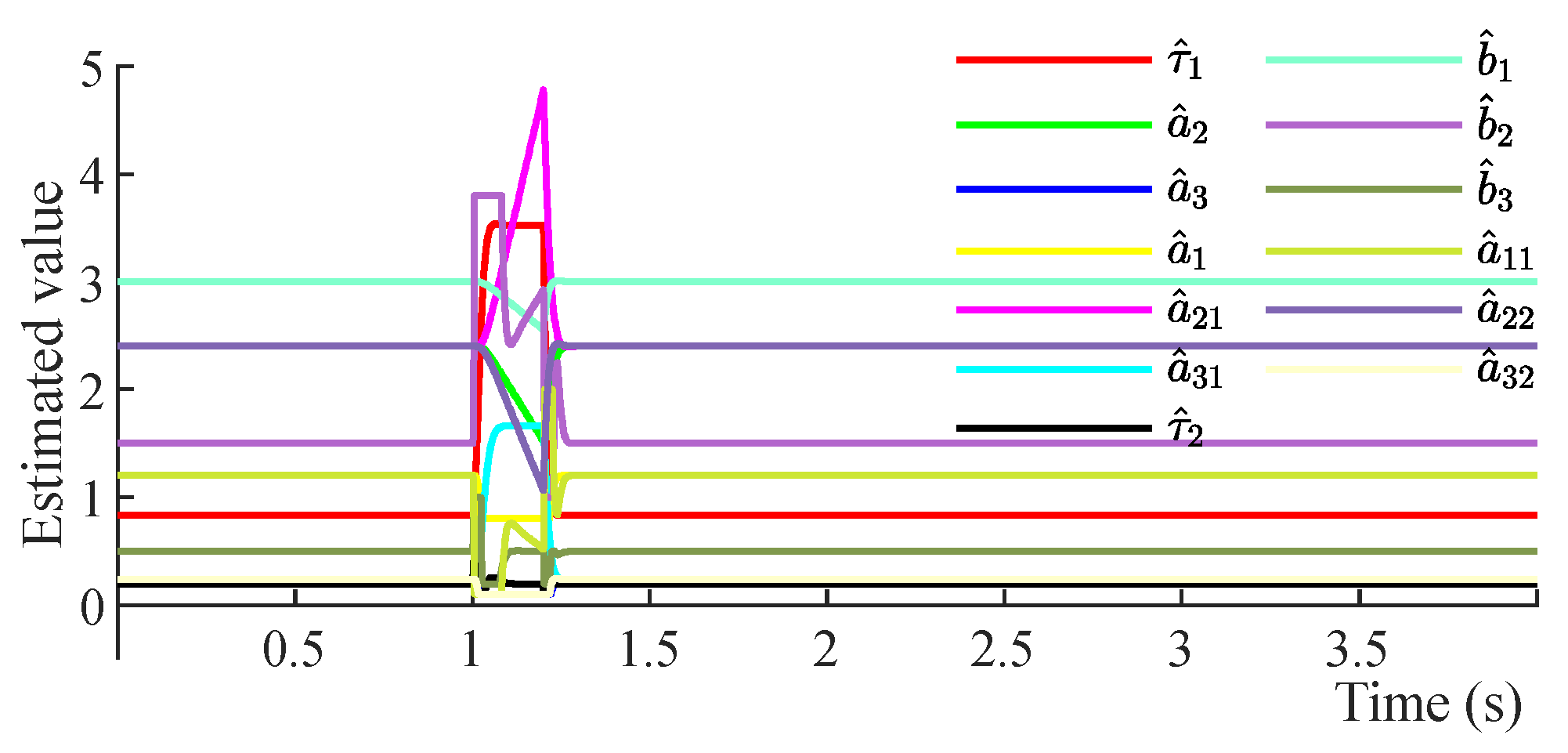
- The unknown disturbance and parameter uncertainty of the EHB gear-drive servo system are considered. In this paper, the parameter-updating law is designed for each parameter in view of the parameter uncertainty in the system. In order to compensate for the unknown disturbance, the boundary estimates are introduced into the parameter-updating law and the control law.
- (2)
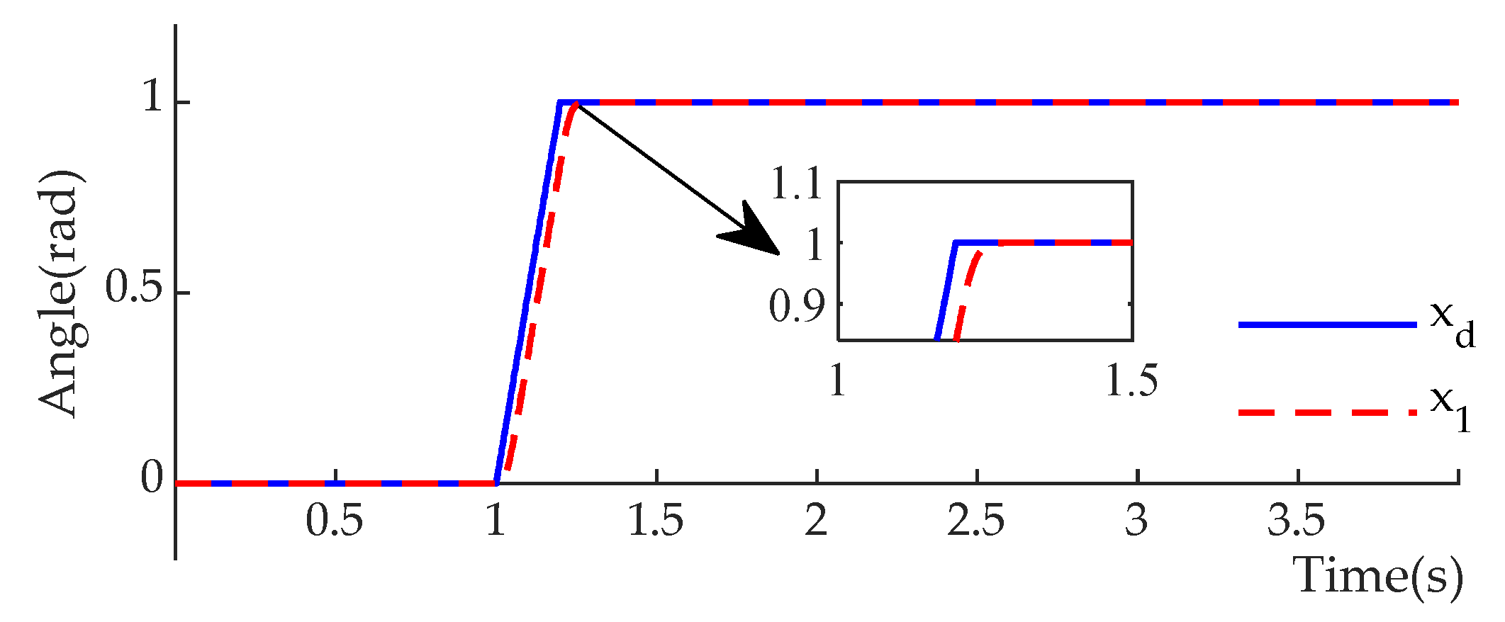
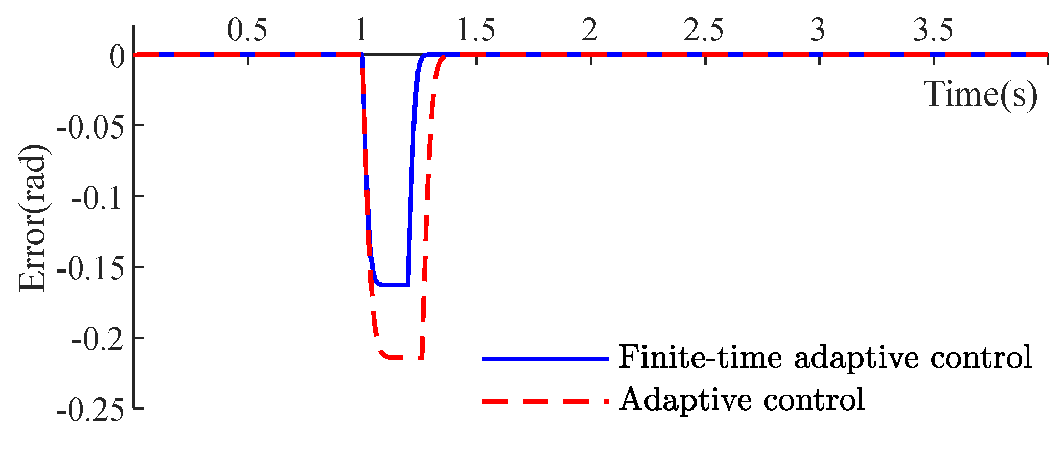
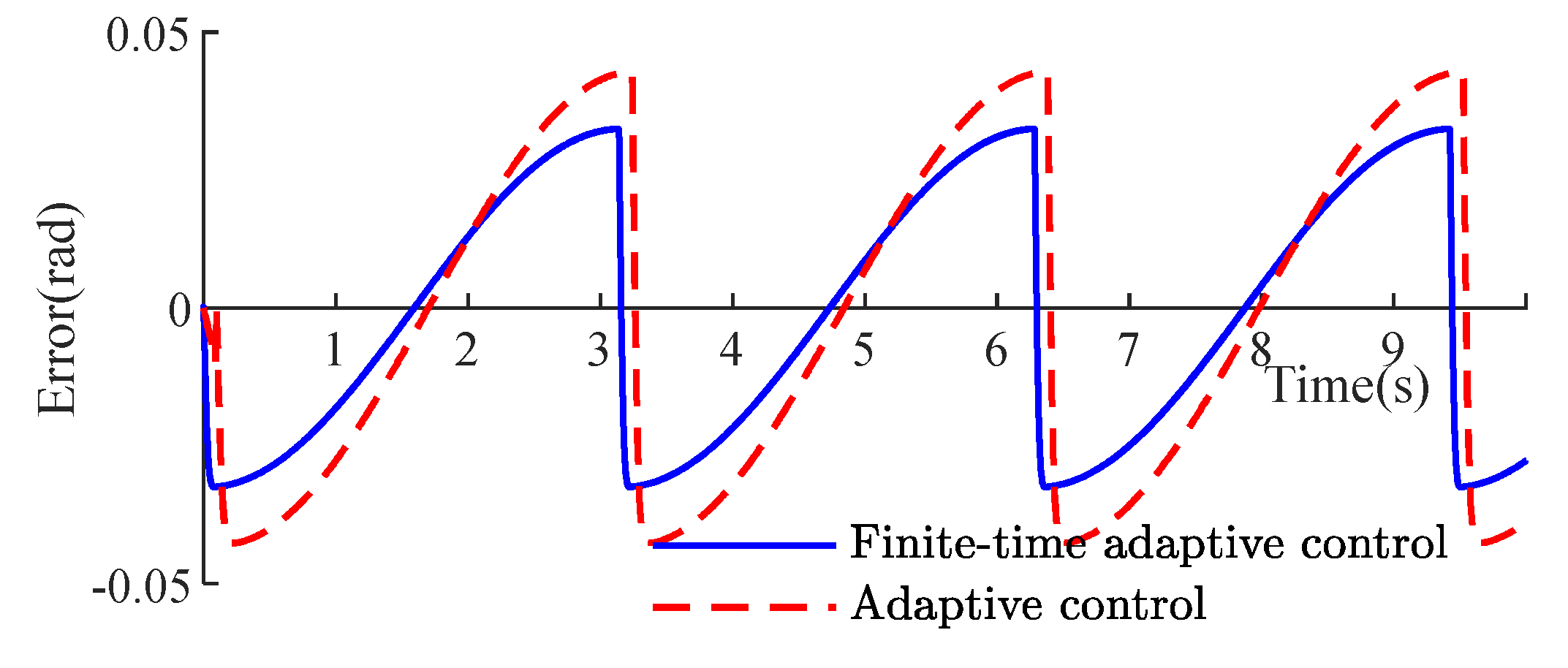
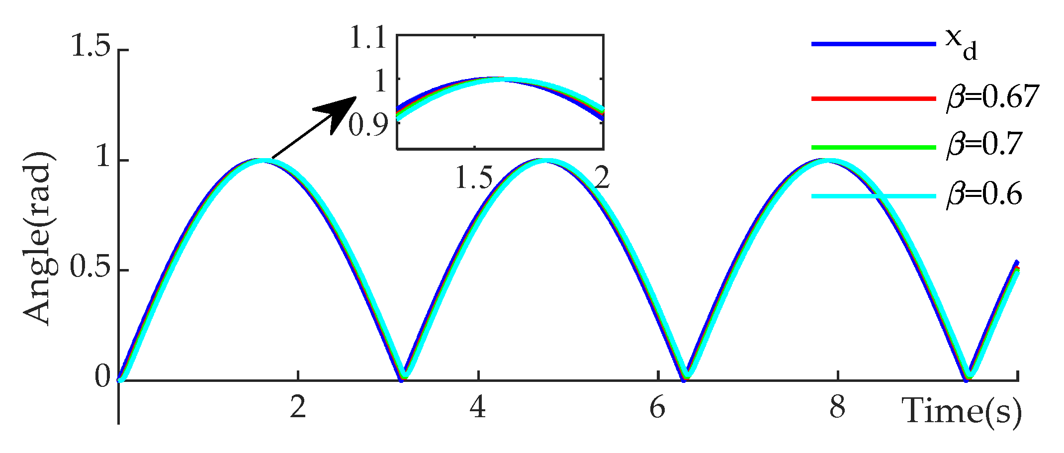
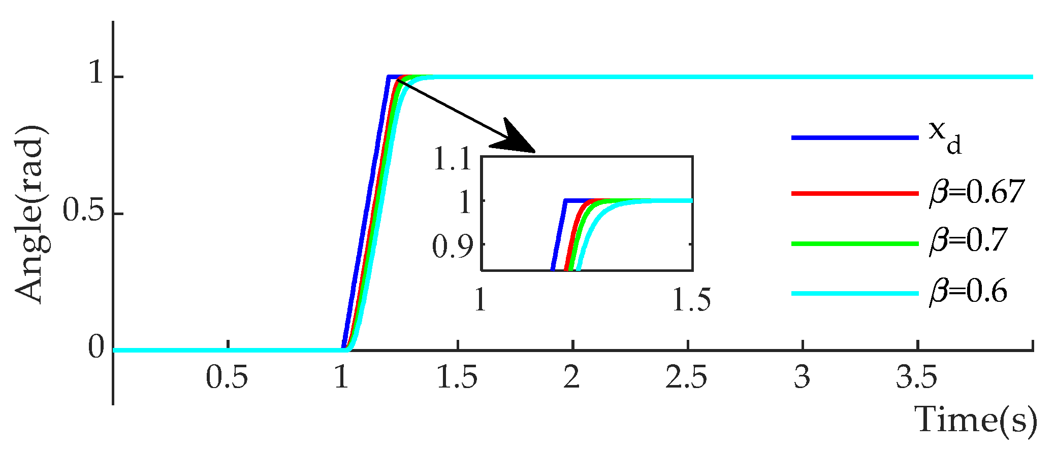
- In order to improve the convergence rate of the system, this paper combines the adaptive control theory with the finite-time control theory to introduce the power exponent β. By adjusting the value of β, the system error can be guaranteed to converge to a certain range in a limited time.
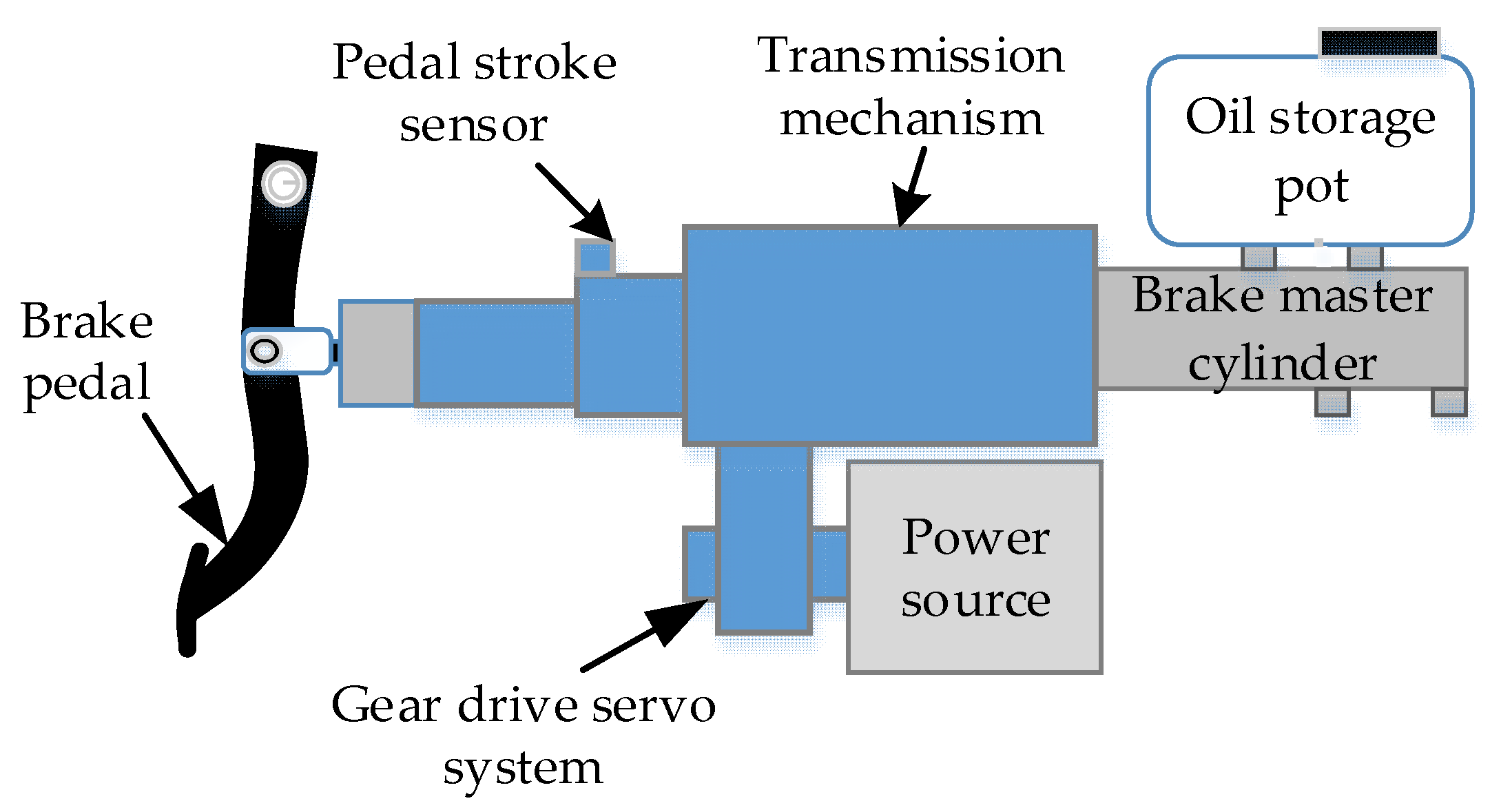
2. System Modeling
3. Controller Designing and Stability Analysis
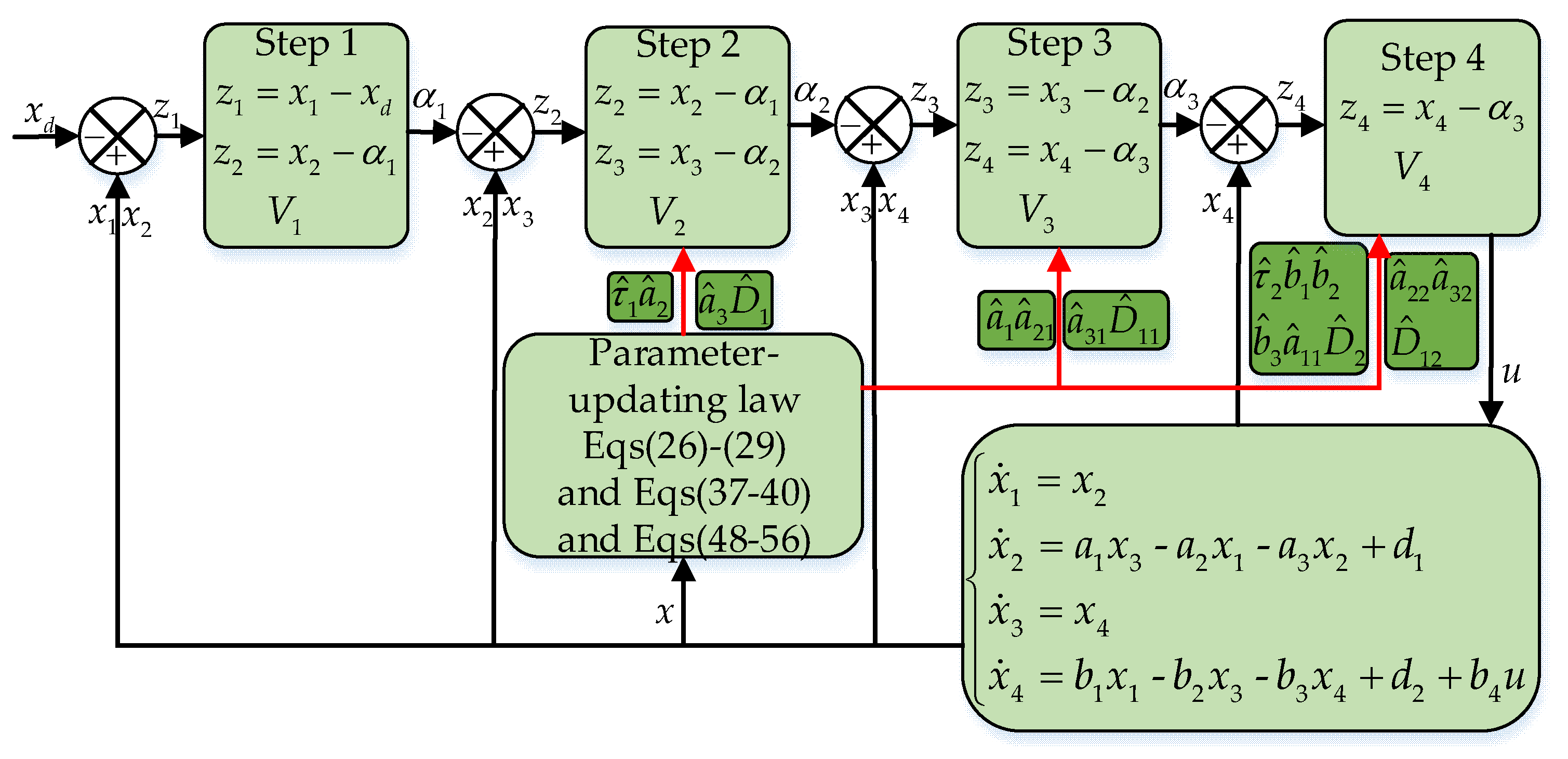
3.1. Design of Adaptive Controller
3.2. Stability Analysis
- (1)
- is positive definite.
- (2)
- The existence of positive real numbers and , and the existence of an open neighborhood containing the origin, makes the following true:If , then it is globally finitely time-stable.
4. Simulation Results and Discussion
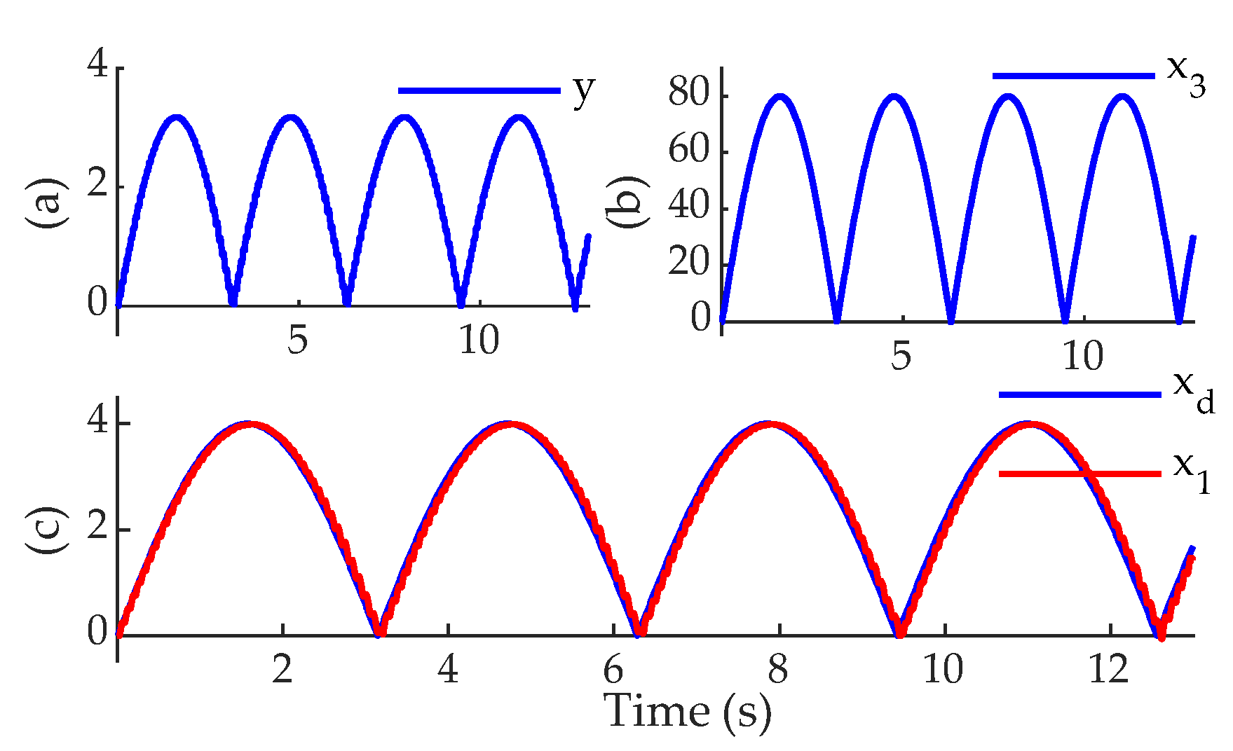
4.1. Experiment 1
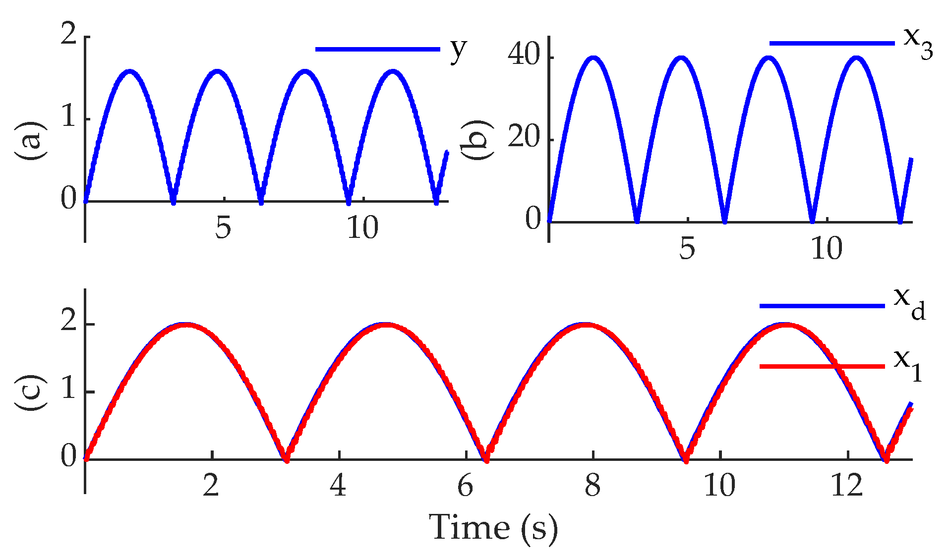
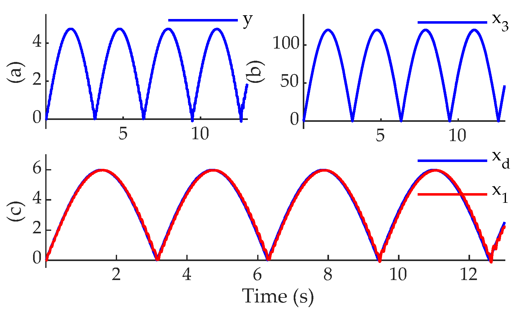
4.2. Experiment 2
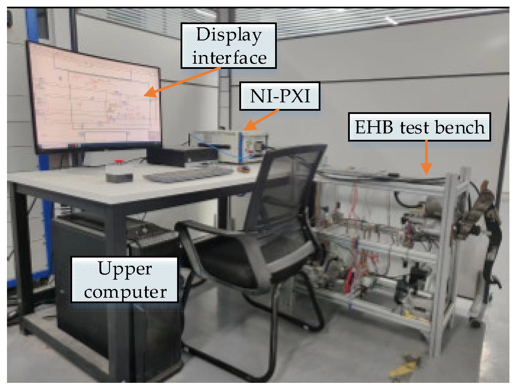
5. Implementation and Results of the HIL Test
6. Conclusions
Author Contributions
Funding
Data Availability Statement
Conflicts of Interest
References
- Xiang, W.; Richardson, P.C.; Zhao, C.; Mohammad, S. Automobile brake-by-wire control system design and analysis. IEEE Trans. Veh. Technol. 2008, 57, 138–145. [Google Scholar] [CrossRef]
- Milanés, V.; González, C.; Naranjo, J.E.; Onieva, E.; De Pedro, T. Electro-hydraulic braking system for autonomous vehicles. Int. J. Automot. Technol. 2010, 11, 89–95. [Google Scholar] [CrossRef]
- Yeo, H.; Koo, C.; Jung, W.; Kim, D.; Cheon, J.S. Development of Smart Booster Brake Systems for Regenerative Brake Cooperative Control; 0148-7191; SAE Technical Paper; SAE International: Warrendale, PA, USA, 2011. [Google Scholar]
- Feigel, H.-J. Integrated brake system without compromises in functionality. ATZ Worldw. 2012, 114, 46–50. [Google Scholar] [CrossRef]
- Tan, Z.-H.; Chen, Z.-F.; Pei, X.-F.; Guo, X.-X.; Pei, S.-H. Development of integrated electro-hydraulic braking system and its ABS application. Int. J. Precis. Eng. Manuf. 2016, 17, 337–346. [Google Scholar] [CrossRef]
- Yu, Z.; Xu, S.; Xiong, L.; Han, W. An Integrated-Electro-Hydraulic Brake System for Active Safety; 0148-7191; SAE Technical Paper; SAE International: Warrendale, PA, USA, 2016. [Google Scholar]
- Zhao, J.; Hu, Z.; Zhu, B. Pressure Control for Hydraulic Brake System Equipped with an Electro-Mechanical Brake Booster; 0148-7191; SAE Technical Paper; SAE International: Warrendale, PA, USA, 2018. [Google Scholar]
- Liu, S.; Zhang, L.; Niu, B.; Zhao, X.; Ahmad, A.M. Adaptive neural finite-time hierarchical sliding mode control of uncertain under-actuated switched nonlinear systems with backlash-like hysteresis. Inf. Sci. 2022, 599, 147–169. [Google Scholar] [CrossRef]
- Cao, Z.; Niu, B.; Zong, G.; Xu, N. Small-gain technique-based adaptive output constrained control design of switched networked nonlinear systems via event-triggered communications. Nonlinear Anal. Hybrid Syst. 2023, 47, 101299. [Google Scholar] [CrossRef]
- Theodorakopoulos, A.; Rovithakis, G.A. Guaranteeing preselected tracking quality for uncertain strict-feedback systems with deadzone input nonlinearity and disturbances via low-complexity control. Automatica 2015, 54, 135–145. [Google Scholar] [CrossRef]
- Tarbouriech, S.; Prieur, C.; Queinnec, I. Stability analysis for linear systems with input backlash through sufficient LMI conditions. Automatica 2010, 46, 1911–1915. [Google Scholar] [CrossRef]
- Li, M.; Chen, H.; Zhang, R. An input dead zones considered adaptive fuzzy control approach for double pendulum cranes with variable rope lengths. IEEE/ASME Trans. Mechatron. 2022, 27, 3385–3396. [Google Scholar] [CrossRef]
- Margielewicz, J.; Gąska, D.; Litak, G. Modelling of the gear backlash. Nonlinear Dyn. 2019, 97, 355–368. [Google Scholar] [CrossRef]
- Vörös, J. Modeling and identification of systems with backlash. Automatica 2010, 46, 369–374. [Google Scholar] [CrossRef]
- Corradini, M.L.; Manni, A.; Parlangeli, G. Variable structure control of nonlinear uncertain sandwich systems with nonsmooth nonlinearities. In Proceedings of the 2007 46th IEEE Conference on Decision and Control, New Orleans, LA, USA, 12–14 December 2007; pp. 2023–2028. [Google Scholar]
- Shi, Z. Global asymptotic tracking for gear transmission servo systems with differentiable backlash nonlinearity. In Proceedings of the 2014 Seventh International Symposium on Computational Intelligence and Design, Hangzhou, China, 13–14 December 2014; pp. 253–257. [Google Scholar]
- Shi, Z.; Zuo, Z. Backstepping control for gear transmission servo systems with backlash nonlinearity. IEEE Trans. Autom. Sci. Eng. 2014, 12, 752–757. [Google Scholar] [CrossRef]
- Zuo, Z.; Ju, X.; Ding, Z. Control of gear transmission servo systems with asymmetric deadzone nonlinearity. IEEE Trans. Control Syst. Technol. 2015, 24, 1472–1479. [Google Scholar] [CrossRef]
- Shi, Z.; Zuo, Z.; Liu, H. Backstepping control for gear transmission servo systems with unknown partially nonsymmetric deadzone nonlinearity. Proc. Inst. Mech. Eng. Part C J. Mech. Eng. Sci. 2017, 231, 2580–2589. [Google Scholar] [CrossRef]
- Lewis, F.L.; Tim, W.K.; Wang, L.-Z.; Li, Z. Deadzone compensation in motion control systems using adaptive fuzzy logic control. IEEE Trans. Control Syst. Technol. 1999, 7, 731–742. [Google Scholar] [CrossRef]
- Zhou, J.; Wen, C.; Zhang, Y. Adaptive output control of nonlinear systems with uncertain dead-zone nonlinearity. IEEE Trans. Autom. Control 2006, 51, 504–511. [Google Scholar] [CrossRef]
- Li, Y.; Tong, S. Adaptive fuzzy output-feedback control of pure-feedback uncertain nonlinear systems with unknown dead zone. IEEE Trans. Fuzzy Syst. 2013, 22, 1341–1347. [Google Scholar] [CrossRef]
- He, X.; Lou, B.; Yang, H.; Lv, C. Robust decision making for autonomous vehicles at highway on-ramps: A constrained adversarial reinforcement learning approach. IEEE Trans. Intell. Transp. Syst. 2022, 24, 4103–4113. [Google Scholar] [CrossRef]
- He, X.; Yang, H.; Hu, Z.; Lv, C. Robust lane change decision making for autonomous vehicles: An observation adversarial reinforcement learning approach. IEEE Trans. Intell. Veh. 2022, 8, 184–193. [Google Scholar] [CrossRef]
- Javaid, U.; Dong, H.; Ijaz, S.; Alkarkhi, T.; Haque, M. High-performance adaptive attitude control of spacecraft with sliding mode disturbance observer. IEEE Access 2022, 10, 42004–42013. [Google Scholar] [CrossRef]
- Xie, B.; Wang, W.; Zuo, Z. Adaptive output feedback control of uncertain gear transmission system with dead zone nonlinearity. In Proceedings of the 2018 13th IEEE Conference on Industrial Electronics and Applications (ICIEA), Wuhan, China, 31 May–2 June 2018; pp. 438–443. [Google Scholar]
- Song, J.; Zuo, Z.; Ding, Z. Adaptive backstepping control of gear transmission systems with elastic deadzone. In Proceedings of the 2017 36th Chinese Control Conference (CCC), Dalian, China, 26–28 July 2017; pp. 878–883. [Google Scholar]
- Wang, S.; Fan, Z.; Li, B.; Tang, X.; Chen, Z.; Zhou, Q.; Wu, J. Research on adaptive control of input time delay for vehicle electronic stability control system. In Proceedings of the 2022 6th CAA International Conference on Vehicular Control and Intelligence (CVCI), Nanjing, China, 28–30 October 2022; pp. 1–5. [Google Scholar]
- Wu, L.-B.; Park, J.H.; Xie, X.-P.; Liu, Y.-J.; Yang, Z.-C. Event-triggered adaptive asymptotic tracking control of uncertain nonlinear systems with unknown dead-zone constraints. Appl. Math. Comput. 2020, 386, 125528. [Google Scholar] [CrossRef]
- Hua, C.; Li, Y.; Guan, X. Finite/fixed-time stabilization for nonlinear interconnected systems with dead-zone input. IEEE Trans. Autom. Control 2016, 62, 2554–2560. [Google Scholar] [CrossRef]
- Bao, J.; Wang, H.; Liu, P.X. Finite-time synchronization control for bilateral teleoperation systems with asymmetric time-varying delay and input dead zone. IEEE/ASME Trans. Mechatron. 2020, 26, 1570–1580. [Google Scholar] [CrossRef]
- Yao, D.; Dou, C.; Zhao, N.; Zhang, T. Finite-time consensus control for a class of multi-agent systems with dead-zone input. J. Frankl. Inst. 2021, 358, 3512–3529. [Google Scholar] [CrossRef]
- Wang, W.; Xie, B.; Zuo, Z.; Fan, H. Adaptive backstepping control of uncertain gear transmission servosystems with asymmetric dead-zone nonlinearity. IEEE Trans. Ind. Electron. 2018, 66, 3752–3762. [Google Scholar] [CrossRef]
- Yin, S.; Shi, P.; Yang, H. Adaptive fuzzy control of strict-feedback nonlinear time-delay systems with unmodeled dynamics. IEEE Trans. Cybern. 2015, 46, 1926–1938. [Google Scholar] [CrossRef]
- Wu, J.; Zhang, J.; Nie, B.; Liu, Y.; He, X. Adaptive control of PMSM servo system for steering-by-wire system with disturbances observation. IEEE Trans. Transp. Electrif. 2021, 8, 2015–2028. [Google Scholar] [CrossRef]
- He, X.; Wu, J.; Huang, Z.; Hu, Z.; Wang, J.; Sangiovanni-Vincentelli, A.; Lv, C. Fear-neuro-inspired reinforcement learning for safe autonomous driving. IEEE Trans. Pattern Anal. Mach. Intell. 2023, 1–13. [Google Scholar] [CrossRef]
- Lu, W.; Liu, X.; Chen, T. A note on finite-time and fixed-time stability. Neural Netw. 2016, 81, 11–15. [Google Scholar] [CrossRef]
- Li, X.; Yang, X.; Song, S. Lyapunov conditions for finite-time stability of time-varying time-delay systems. Automatica 2019, 103, 135–140. [Google Scholar] [CrossRef]


| Symbol | Parameter | Value | Units |
|---|---|---|---|
| moment of inertia of the driven side | 0.52 | kg·m2 | |
| driving side moment of inertia | 0.21 | kg·m2 | |
| viscous friction on the driven side | 0.124 | Nm/rad | |
| driving side viscous friction coefficient | 0.11 | Nm/rad | |
| stiffness coefficient | 0.33 | Nm/rad | |
| break point | 0.062 | rad | |
| break point | 0.051 | rad |
Disclaimer/Publisher’s Note: The statements, opinions and data contained in all publications are solely those of the individual author(s) and contributor(s) and not of MDPI and/or the editor(s). MDPI and/or the editor(s) disclaim responsibility for any injury to people or property resulting from any ideas, methods, instructions or products referred to in the content. |
© 2023 by the authors. Licensee MDPI, Basel, Switzerland. This article is an open access article distributed under the terms and conditions of the Creative Commons Attribution (CC BY) license (https://creativecommons.org/licenses/by/4.0/).
Share and Cite
Wang, S.; Cao, Q.; Ma, F.; Wu, J. EHB Gear-Drive Symmetric Dead-Zone Finite-Time Adaptive Control. Machines 2023, 11, 1002. https://doi.org/10.3390/machines11111002
Wang S, Cao Q, Ma F, Wu J. EHB Gear-Drive Symmetric Dead-Zone Finite-Time Adaptive Control. Machines. 2023; 11(11):1002. https://doi.org/10.3390/machines11111002
Chicago/Turabian StyleWang, Shuai, Qinghua Cao, Fukuo Ma, and Jian Wu. 2023. "EHB Gear-Drive Symmetric Dead-Zone Finite-Time Adaptive Control" Machines 11, no. 11: 1002. https://doi.org/10.3390/machines11111002
APA StyleWang, S., Cao, Q., Ma, F., & Wu, J. (2023). EHB Gear-Drive Symmetric Dead-Zone Finite-Time Adaptive Control. Machines, 11(11), 1002. https://doi.org/10.3390/machines11111002