A New Exoskeleton Prototype for Lower Limb Rehabilitation ^†

Abstract

This paper presents a new solution for an exoskeleton robotic system that is used for locomotor assistance in people with locomotor disabilities. As novel features of the present research, a novel structural solution of a plane-parallel kinematic chain, intended to be used as the leg of an exoskeleton robot, is proposed. A virtual prototype is made, on the basis of which kinematic and dynamic studies are carried out using ADAMS software for the dynamic analysis of multibody systems. The dynamic simulation of the exoskeleton is performed in two simulation situations: walking on a horizontal plane, as well as the simulation of motion assistance when climbing stairs. Following this analysis, it is noted that the robotic system achieves angular variations in the hip and knee joints similar to that of a human subject. As a result, the constructive solution is feasible, and the next stage of the study is to realize an experimental prototype by the rapid prototyping technique. The kinematic elements of the exoskeleton are designed to provide structural strength, to be easily manufactured by 3D printing and to be easy to assemble. For this purpose, the structural optimization is performed with the finite element method to eliminate stress concentrators. Finally, an experimental prototype of the exoskeleton robot is manufactured and assembled, whose motion is analyzed using ultrafast-camera-based video analysis.

1. Introduction

An exoskeleton [1] (from Greek external and skeleton) is an external mechanical system that contributes to human strength, especially during movement. Productivity-enhancing exoskeletons are designed to give healthy people the ability to perform complex tasks more easily or tasks that otherwise cannot be performed, but there are also exoskeletons used for medical purposes to help patients with disorders of the musculoskeletal system. By placing the sensors, the condition of the human body can be monitored, as well as the movements of limbs and muscles. Based on the data obtained from the sensors and a mathematical model describing the movements of the human body, implemented in a computer program, the exoskeleton can be controlled. Most invertebrates have exoskeletons in the form of shells (many protozoans, mollusks) or cuticles (the chitinous shell of arthropods). Arthropods are the most prosperous group of living organisms, with their number of species exceeding the number of species of all other animals combined [1].

It can be said that man was inspired in the creation of the exoskeleton by nature, continuously perfecting mechanical systems of this type until today; new versions of exoskeletons are even made by leading companies in the world. The Russian inventor Nikolai Ferdinandovich Yagn (Nicholas Yagn), who lived in America, registered a series of patents on the exoskeleton in 1890 [2]. These are considered the earliest mentions of the exoskeleton. The mechanical exoskeleton systems he patented were intended mainly for soldiers to facilitate walking, running and jumping; this device was never built.

A major contribution to the development of exoskeletons was also made by fiction novels, such as Robert Heinlein’s 1959 military science fiction novel Starship Troopers.

In 1960, General Electric Research, in collaboration with researchers at Cornell University and with financial support from the US Office of Naval Research, began designing and building the first prototype of a full-body exoskeleton, called the “Hardiman”, weighing up to 80 kg [1]; it could lift up to 680 kg and was intended for use in military arsenals, for large-caliber aviation ammunition, underwater and in space, and in nuclear power plants; however, tests in 1965 rejected its use.

In 1960–1961, Niel J. Mizen created the exoskeleton “The Man Amplifier” [3] in the Cornell Aeronautical Lab; hydraulic and electric motors were applied in the main couplings of the mechanical system; however, it was difficult to operate and expensive, which is why it was not released to industry or the public.

No major breakthroughs or achievements were made in the following period, but related branches were developed and knowledge and experience were gained.

One of the first exoskeletons (HAL) affordable to the public market was proposed by Yoshiyuki Sankai of Cybernics in 1992. In [4], three systems are presented evolutionarily. HAL has two settings: voluntary cybernetic control and autonomous cybernetic control. When a bioelectric signal is detected, the suit calculates the additional torque required to drive the kinematic couplings. The exoskeleton robot has multiple uses such as: capacity building for able-bodied people, support for hard work, rehabilitation and entertainment.

In 2001, the Defense Advanced Research Projects Agency (DARPA) of the Department of Defense began a seven-year program to develop their Exoskeletons for Human Performance Augmentation program. Projects from 14 companies and universities were considered, but only the following were selected: Sarcos Research Corporation, the University of California at Berkeley and Oak Ridge National Laboratory. Since 2004, Sarcos Research Corporation, later acquired by Raytheon, has been the prime contractor for the development of fast, armored and powerful exoskeletal systems.

The research into exoskeletons is ongoing and is a current area of study. A special category of exoskeletons are mechanical walking systems, used for the rehabilitation of patients with musculoskeletal disorders. Providing stability in the single-leg support phase is not straightforward, which is why mobile frames can be attached.

Walking robots have certain advantages and disadvantages [5,6,7,8,9,10,11].

Advantages: can move over difficult terrain; intermittent contact with the ground; the trajectory of the robot body is decoupled from the trajectory of the legs; the position of the transported load is not influenced by irregularities in the ground; can climb stairs, and avoid obstacles; can vary leg lengths (active suspension); are suitable for the human environment.

Disadvantages: complex mechanical system; high energy consumption; complex control algorithms; low speed on rough terrain; synchronization of the operation of a large number of kinematic couplings.

In bi-directional robots, foot coordination is simpler, requiring control of only two contact surfaces. They can also move in narrow spaces and consume less energy.

The first ideas for the implementation of legged vehicles appear in the 15th century (1495–1497), in the writings of Leonardo da Vinci (“the mechanical knight”). Da Vinci’s “mechanical knight” is considered to be the first humanoid robot created; it was constructed of wood, with leather and bronze elements, and operated by cables. Replicas of da Vinci’s robot were built in 2002 and 2007, and its capabilities were confirmed: it could move its arms and legs, sit and stand, move its neck and raise its visor. Da Vinci’s design was used by NASA to help build planetary exploration robots and still inspires robotics researchers today.

In 1850, Chebyshev made a walking mechanism in which the body moved horizontally and the legs moved up and down, alternately making contact with the ground. The curves traced by the base of the foot were of the “flattened D” type [12].

From 1950 onwards, the research on walking machines by various research groups intensified. In 1960, Shigley published a paper with numerous bar and cam mechanisms, applicable to walking devices. After this date, corporations such as Space General Corporation built various walking machines with various facilities. More complex walking vehicles were also made, but their control by the operator was heavy (e.g., the General Electric patrol car, designed by R. Moshler), requiring the use of computers [13].

The first computer-controlled, self-propelled quadruped, Phoney Poney, was developed by McGhee and Frank in 1966. The walking robot was capable of two types of gaits but only in a straight line [14].

Robotics for rehabilitation treatment is an emerging field that is expected to grow as a solution for rehabilitation automation [15,16]. Robotic rehabilitation can: replace the physical training effort of a therapist, allowing for more intense repetitive movements and providing therapy at a reasonable cost; and quantitatively assess the level of motor recovery by measuring force and movement trajectories [17]. The issues addressed in this paper are related to the kinematic and dynamic analysis of exoskeleton robotic systems intended for the rehabilitation of people with locomotor disabilities. This category of mobile robotic systems has undergone two directions of development: the development of open kinematic chains with motors placed in the system joints and the development of closed kinematic chains with a single drive motor [18]. In the last decade, several robotic lower limb rehabilitation systems have been developed to restore mobility to affected limbs. These systems can be grouped according to the rehabilitation principle, and they follow: treadmill systems with patient suspension system; underfoot plate-based gait systems; ground-based gait systems, stationary systems, chair-based systems and ankle rehabilitation systems [19]. Studies on the experimental determination of the laws of motion performed in the human gait on stairs are presented in [15]. As a novelty, we found from the literature study that systems with a dual functional role have been developed, as a gait trolley and as an exoskeleton for assisting upright position and gait [20].

The stair motion assistance with an exoskeleton topic is present in the field of electronics and addresses the problem of cooperative control between the exoskeleton and the human subject or for reducing energy consumption when climbing stairs [21,22,23,24,25,26]. Preliminary evaluations are performed for this topic [27], as well as analyses of fall possibilities [28,29,30]. The situation of stair descent by means of assistance with an exoskeleton or improvement of stair climbing abilities by means of an exoskeleton actuated by myoelectric muscle signals is also addressed in the literature [31,32,33,34].

The paper is structured in four parts. After the “Introduction”, an experimental study of the biomechanics of human gait is presented, where the laws of variation in angles in the joints of the human foot are experimentally established. Next, the structure, kinematics and dynamics of the robotic system proposed for rehabilitation are presented. In the last part a test of the experimental prototype of the robotic system is performed.

2. Human Gait Experimental Study

This study is necessary to experimentally establish the laws of variation in flexion/extension angles in the joints of the human foot. Later, these laws will be used as a benchmark for those achieved by the robotic system. During a normal gait, angular variations occur in the foot joints in both the sagittal and frontal planes. The vast majority of robotic rehabilitation systems perform movements only in the sagittal plane, as is the case with the structure presented in this paper. For this reason, we will only analyze the laws of variation in flexion/extension angles in the joints, namely, in the sagittal plane. These laws are determined experimentally using goniometer-type sensors.

To obtain the kinematic parameters of human gait we used the Biometrics Ltd. data acquisition system, which is based on electrogoniometer-type sensors. This system is widely used in biomechanics, due to the fact that the sensors are connected to a device that transmits the data via Bluetooth interface to a laptop computer. To record angular variations in the leg joints, six electrogoniometers were used, which are fixed with double adhesive tape on the respective joint, as shown in Figure 1. Measurements are made at a frequency of 500 Hz.

In this research, we present the results obtained for the average cycle related to a normal gait for the subject: a healthy male of 1.68 m height, 68 kg and age 35, shown in Figure 1.

The variation laws for the flexion–extension angle in the ankle joint, shown in Figure 2, and the flexion–extension angles for the knee and hip joints, shown in Figure 3 and Figure 4, are, thus, obtained. The human gait is a repetitive process that shows variability from individual to individual. The results shown represent the laws of variation for one gait cycle.

The gait cycle can be split down into two primary phases, the stance and swing phases, which alternate for each lower limb. The stance phase means the entire time that a foot is on the ground. The swing phase represents the entire time that the foot is in the air.

As can be seen from the results obtained for the knee joint, the angular amplitude is 55 degrees, and for the hip joint, it is 30 degrees. These angular amplitudes must also be achieved by the designed exoskeleton. The experimentally obtained laws for the human gait are compared with those achieved by the exoskeleton.

3. Optimal Design and Simulation Study of the Proposed Structural Solution for the Exoskeleton Leg

The consideration taken into account in the development of the structural solution is that it should be a low-cost solution. For this reason, the foot structure comprises two kinematic elements that structurally model the femur and tibia bones, as well as two rotational joints that structurally model the knee and hip joints. The ankle joint is not actuated, as the developed solution is intended to be a low-cost one, this joint is designed so as to include a torsion spring in the structure. The feasibility of the proposed structural solutions are verified by virtual simulation, aiming to obtain variation laws similar to those achieved by a healthy human subject in the knee and hip joints of the foot mechanism. Obviously, according to other studies [35], the trajectory performed by the ankle joint must be ovoid. Moreover, the portion corresponding to the propulsion phase of the exoskeleton must be linear. With these considerations, we have developed three structural solutions, which are shown in Figure 5.

Thus, in Figure 5a—a structural solution is shown, where element 5 acts as a femur and element 7, through the IM segment, acts as a tibia. The femur and tibia are connected by the I-coupling, which structurally shapes the knee joint. The H-coupling models the hip joint in the structure of the human leg. This structure was analyzed and presented in the paper [35]. Since its structure is based on an articulated quadrilateral-type contour driven by element 2 of a Chebyshev-type kinematic chain, similar angular variations are obtained in the hip and knee joints, while in a normal gait in the knee joint, the angular amplitude must be double. It can be used for rehabilitation for certain patients who require rehabilitation with reduced angular amplitude. In Figure 5 there are noted the kinematic couplings of the mechanisms with capital letters, and with numbers from 1 to 7 or 9 there are noted the kinematic elements of the mechanisms. The coupling H is a multiple coupling, namely: the coupling H is a rotational coupling between kinematic element 4 and element 5, and H* between element 4 and the base.

In order to achieve solutions with movements closer to the human foot, it is proposed to introduce a kinematic chain of the articulated quadrilateral type in the knee joint, as shown in Figure 5b,c [36,37].

The other two solutions have in their structure 7 kinematic elements and 10 rotational couplings, respectively, 9 elements and 14 couplings. For the solution in Figure 5b, elements 4 and 7 materialize the femur and tibia bones, and the D and J couplings materialize the hip and knee joints. This solution has in its structure a kinematic chain of the articulated quadrilateral type, GHIJ, acting on the knee joint. The movement of the whole structure is achieved by the articulated quadrilateral kinematic chain ABCD.

In the solution of Figure 5c, the actuation is performed by means of the Lambda Chebyshev kinematic chain, consisting of elements 1, 2 and 3. The driving element has two arms offset by 180°, imparting antiphase operation to the two kinematic chains; the linkage curves made by the end elements of the kinematic chains, as well as their counter-timing, contribute to the biped walking.

In conclusion, two original structural solutions are proposed for study, one with 7 elements and the other with 9 kinematic elements. In this paper, we study, by numerical simulation and experiment, the structural solution with 7 kinematic elements, shown in Figure 5b.

The purpose for which the robotic exoskeleton systems were developed is to assist people with locomotor disabilities to walk. For this reason, it is intended that the movement performed by the robot’s leg mechanism should be similar to that of a human subject. People who have suffered a stroke require support from an assistive robot for gait rehabilitation. For this reason, the solution presented in Figure 5c is studied.

Among the advantages of the new structural solution, we can highlight the following: the drive part is placed further back than the kinematic chain of the foot, in this way being a more ergonomic solution, easier to wear by humans; the angle variation laws of the hip and knee joints have amplitudes very close to those of the human, for a normal gait; the stride length is greater than in the previous solution.

3.1. Kinematic Analysis of the Foot Mechanism

The positions of the couplings and angles of the kinematic elements are determined using the vector contour method in the order indicated in the decomposition according to Assur’s principle. The vector sums are projected onto the axes of the reference system, and the equations are written in the MAPLE 12 program, obtaining values for the positions of the points and angles of the driving element and the three dyads. These equations and the results obtained are presented in detail below, based on the scheme from Figure 6.

For the first structural group (Dyad BCD), the following equation is written

$$\begin{array}{c}\overline{AC}=\overline{AB}+\overline{BC}=\overline{AD}+\overline{DC}\\ \left\{\begin{array}{c}{x}_C=x_B+l_{BC}\cdot \mathit{cos}{\alpha }_2=x_D+l_{CD}\cdot \mathit{cos}{\alpha }_3\\ y_C=y_B+l_{BC}\cdot \mathit{sin}{\alpha }_2=y_D+l_{CD}\cdot \mathit{sin}{\alpha }_3\end{array}\right.\end{array}$$

(1)

The unknowns in the previous system are $x_C,y_C,{\alpha }_2,{\alpha }_3$. For the 90-degree angle of the leading element, these unknowns take on the values: $x_C=175.3737 \mathrm{m}\mathrm{m}$, $y_C=-76.1460 \mathrm{m}\mathrm{m}$, ${\alpha }_2=331.26691°$, ${\alpha }_3=270.000526°$.

For the second structural group (Dyad EFG), the following equation is written

$$\begin{array}{c}\overrightarrow{AF}=\overrightarrow{AE}+\overrightarrow{EF}=\overrightarrow{AG}+\overrightarrow{GF}\\ \left\{\begin{array}{c}{x}_F=x_E+l_{EF}\cdot \mathit{cos}{\alpha }_4=x_G+l_{GF}\cdot \mathit{cos}{\alpha }_5\\ y_F=y_E+l_{EF}\cdot \mathit{sin}{\alpha }_4=x_G+l_{GF}\cdot \mathit{sin}{\alpha }_5\end{array}\right.\end{array}$$

(2)

The mechanism can be divided according to Assur’s principle into a rotating driving element and 6 RRR dyads: BCD, EFG, HIJ, B’C’D’, E’F’G’ and H’I’J’ (Figure 7).

In Figure 7 there are noted the kinematic couplings of the mechanism structural groups with capital letters, and with numbers from 1 to 7 there are noted the kinematic elements of the mechanism.

The unknowns in the previous system are $x_F,y_F,{\alpha }_4,{\alpha }_5$. For the 90-degree angle of the leading element, these unknowns take on the values: $x_F=118.8561 \mathrm{m}\mathrm{m}$,$y_F=-417.4430 \mathrm{m}\mathrm{m}$, ${\alpha }_4=272.055827°,{ \alpha }_5=216.153979°$.

For the third structural group (Dyad HIJ), the following equation is written

$$\begin{array}{c}\overrightarrow{AI}=\overrightarrow{AH}+\overrightarrow{HI}=\overrightarrow{AJ}+\overrightarrow{JI}\\ \left\{\begin{array}{c}{x}_I=x_H+l_{HI}\cdot \mathit{cos}{\alpha }_6=x_J+l_{IJ}\cdot \mathit{cos}{\alpha }_7\\ y_I=y_H+l_{HI}\cdot \mathit{sin}{\alpha }_6=y_J+l_{IJ}\cdot \mathit{sin}{\alpha }_7\end{array}\right.\end{array}$$

(3)

The unknowns in the previous system are $x_I,y_I,{\alpha }_6,{\alpha }_7$. For the 90-degree angle of the leading element, these unknowns take on the values: $x_I=75.6531 \mathrm{m}\mathrm{m},y_I=-562.8921 \mathrm{m}\mathrm{m}$, ${\alpha }_6=277.286629°$, ${\alpha }_7=213.794586°$.

The coordinates of the K tracer point are calculated with the relation

$$\begin{array}{c}\overrightarrow{AK}=\overrightarrow{AJ}+\overrightarrow{JK}\\ x_K=x_J+l_{JK}\cdot \mathit{cos}\left({\alpha }_7+\beta \right)\\ y_K=y_J+l_{JK}\cdot \mathit{sin}\left({\alpha }_7+\beta \right)\end{array}$$

(4)

The kinematic analysis presented above is valid for the situation when the system with the two leg mechanisms operates with the upper frame fixed to the base.

3.2. Designing an Optimal CAD Model of the Robotic System

Each kinematic element that goes into the structure of the leg mechanism was designed as a geometric shape and then structurally optimized using an optimization algorithm developed in ANSYS.

Optimization can be defined as the process of maximizing or minimizing a desired objective function with the satisfaction of constraints [37]. Mechanical structures are often analyzed with the finite element method, which is a widely used technique for structural analysis. Finite element analysis is used to analyze the dynamic response and to analyze mechanical strains and stresses in structures that are subjected to loads and boundary conditions. From a mathematical point of view, optimization can be considered a numerical computation technique to analyze problems governed by partial derivative equations, which describe the behavior of the system under study.

The optimization problem based on the finite element method can generally be expressed as: minimize $f(x, U)$, subject to $g_i\left(x, U\right)\le 0$, i = 1,…m, and $h_j\left(x, U\right)=0$ j = 1,…m, where U is the vector of nodal displacements (n dof × 1), for which the field of displacements u (x, y, z) is determined. The relationship between U and x is governed by the equilibrium differential equations: $K\left(x\right)U=F\left(x\right)$.

Where K is the quadratic stiffness matrix (n dof × n dof), and F is the vector of loads (n dof × 1).

Depending on the type of design variables x, finite-element-based optimization may be classified as parameter or size, shape and topology optimization. In parameter or size optimization, the objective function f is typically the weight of the structure, and g_i are the constraints reflecting limits on stress and displacement. The design variable set x can take various forms. The steps taken for structural optimization are described below. Structural optimization involves two main objectives: reducing the mass of the kinematic elements while maintaining the structural integrity of the element and increasing fatigue strength by eliminating mechanical stress concentrators.

The flow chart to achieve the optimal design solution is shown in Figure 8. The parameterization of the design involves specifying geometry dimensions as input parameters, which can vary between certain minimum and maximum values, usually manufacturable values. The mass of the part can also be specified as an input parameter. The initial design solution is analyzed from a structural point of view, and results such as mechanical stress and displacement distribution maps are obtained. These results are specified as output parameters of the optimization process. In the next step of the optimization process, certain constraints are defined (e.g., mechanical stresses not to exceed a certain value) and the objective function is defined. In the case of design optimization, the objective function is the minimization of mass in conjunction with the reduction in mechanical stress concentrators. The “Design of experiment” module is executed, where, by means of an optimization algorithm, the response surfaces are calculated, and the optimal design point is indicated.

The component in ANSYS workbench offers several methods for optimization, such as: screening; a multi-objective genetic algorithm, based on NSGA-II; nonlinear programming by quadratic Lagrangian; mixed integer sequential quadratic programming, adaptive multi-objective method; gradient based adaptive single-objective method.

In the first step, the initial geometry of the element is created in the ANYS Design Modeler preprocessor. Furthermore, at this stage, the geometry parameters are specified that are included in the optimization process as design variables. In this case, the kinematic element geometry is shown in Figure 9, and the geometrical parameters defined as design variables are the radii of the connections named FBlend 8 and FBlend 10, as well as the thickness of the stiffening rib Extrude 8. At this stage, the maximum and minimum geometrically possible values of these parameters must be defined. Between these limits, the manufacturable values that these parameters can take in the optimal design are specified.

For the two connecting radii, the range 2.7–3.3 mm of variation is specified, and for the stiffening rib, the range 10.8–13.2 mm is specified. These parameters of the optimization process are called input parameters. The output parameters are: the resulting elastic displacements: P5—total deformation maximum (mm), the element mass, P6—solid mass (kg), P7—equivalent stress maximum (MPa) and P8—equivalent strain maximum (mm/mm).

The maximum value of the connecting force in the knee kinematic coupling is used as load data, i.e., the value of 2000 N, obtained from dynamic simulation. The output parameters are calculated by performing finite element analysis.

The second stage involved the realization of the study called ”Design of experiments”, central composite design. Based on the data from the study, 15 possible design variants are determined, as shown in

Table 1. Design points of design-of-experiments.

	Param.	Design Point	P11—FBlend8.FD1 (mm)	P12—FBlend10.FD1 (mm)	P13—Extrude8.FD1 (mm)	P6—Solid Mass (kg)	P7—Equivalent Stress Maximum (MPa)
No.
1		1 DP	3	3	12	0.35311	30.143
2		2	2.7	3	12	0.35309	32.611
3		3	3.3	3	12	0.35313	29.84
4		4	3	2.7	12	0.35309	31.317
5		5	3	3.3	12	0.35313	29.047
6		6	3	3	10.8	0.34014	35.815
7		7	3	3	13.2	0.36604	26.465
8		8	2.7561	2.7561	11.024	0.34254	37.626
9		9	3.2439	2.7561	11.024	0.34257	37.534
10		10	2.7561	3.2439	11.024	0.34257	33.137
11		11	3.2439	3.2439	11.024	0.3426	32.682
12		12	2.7561	2.7561	12.976	0.3636	30.394
13		13	3.2439	2.7561	12.976	0.36362	30.318
14		14	2.7561	3.2439	12.976	0.36364	26.646
15		15	3.2439	3.2439	12.96	0.36365	26.498

. For each design point, the output parameters are calculated, as shown in Table 1.

For the output parameters, the minimum and maximum values resulting from the finite element analysis are summarized, as shown in

Table 2. Min–Max Search.

Name	P11—FBlend8.FD1 (mm)	P12—FBlend10.FD1 (mm)	P13—Extrude8.FD1 (mm)	P6—Solid Mass (kg)	P7—Equivalent Stress Maximum (MPa)
Output Parameter Minimums
P5—Total Deformation Maximum	3.3	3.3	13.2	0.36608	24.994
P6—Solid Mass	2.7	2.7	10.8	0.34011	38.982
P7—Equivalent Stress Maximum	3.3	3.3	13.2	0.36608	24.994
P8—Equivalent Elastic Strain Maximum	2.7	3.3	13.2	0.36606	25.568
Output Parameter Maximums
P5—Total Deformation Maximum	27	27	10.8	0.34011	38.982
P6—Solid Mass	3.3	3.3	13.2	0.36608	24.994
P7—Equivalent Stress Maximum	2.7	2.7	10.8	0.34011	38.982
P8—Equivalent Elastic Strain Maximum	3.3	2.7	10.8	0.34015	38.493

.

For the output parameter P6—solid mass, the minimum calculated value is 0.34011 kg, and the maximum is 0.36608 kg. For the output parameter P7—equivalent stress, the minimum calculated value is 24.994 MPa, and the maximum is 38.982 MPa.

In the next step, a response surface is obtained, in the form of a 3D graph, showing the variation of the output parameters in relation to one of the input parameters. The response surface for P5—total deformation maximum, as a function of the three input parameters, is shown in Figure 10.

For the output parameters P6—solid mass, and P7—equivalent stress maximum, the calculated response surfaces are shown in Figure 11 and Figure 12.

The calculation of response surfaces is performed in order to optimize these response surfaces.

Optimization, in this case, involves minimizing the output parameter P6—solid mass and minimizing the parameter P7—equivalent stress maximum. For the parameter P7, a constraint is specified, namely, the maximum value not to exceed 33 MPa, due to material choice considerations.

Table 3. Optimization study.

Optimization study
Minimize P6; P7 ≤ 33 MPa	Goal, minimize P6 (default importance)
Minimize P7	Strict constraint, P7 values less than or equal to 33 MPa (default importance)
Optimization Method
Screening	The Screening optimization method uses a simple approach based on sampling and sorting. It supports multiple objectives and constraints, as well as all types of input parameters. Usually, it is used for preliminary design, which may lead to the application of other methods for more refined optimization results.
Configuration	Generate 8 samples and find 3 candidates.
Status	Converged after 4 evaluations.
Candidate points
	Candidate Point 1	Candidate Point 2	Candidate Point 3
P11—FBlend8. FD1 (mm)	3.3	2.7	3.3
P12—FBlend10. FD2 (mm)	3.3	2.7	3.3
P13—Extrude8.FD1 (mm)	10.8	13.2	13.2
P6—Solid Mass (kg)	*** 0.34019	xxx 0.36602	xxx 0.36608
P7—Equivalent Stress Maximum (MPa)	*** 32.811	*** 30.17	*** 24.994

xxx—not acceptable; ***—acceptable.

shows the optimization goal, namely, the minimization of the input parameters P6 and P7, specifies the optimization method used and presents the three candidate points for the optimal design solution.

It is recommended to choose the solution that is rated with the maximum number of stars for all criteria.

Table 4. Optimization of candidate points.

Name	P11—FBlend8.FD1 (mm)	P12—FBlend10.FD1 (mm)	P13—Extrude8.FD1 (mm)	P6—Solid Mass (kg)		P7—Equivalent Stress Maximum (MPa)
				Parameter Value	Variation from Reference	Parameter Value	Variation from Reference
Candidate Point 1	3.3	3.3	10.8	** 0.34019	−7.07%	** 32.27	31.27%
Candidate Point 2	2.7	2.7	13.2	xxx 0.36602	−0.02%	** 30.17	20.71%
Candidate Point 3	3.3	3.3	13.2	xxx 0.36608	0.00%	** 24.994	0.00%

xxx—not acceptable; **—acceptable.

shows the results obtained for output parameters P6, P7 and P8 for those three design points, the candidate for the optimal solution, or the three design solutions (candidate points). In this case, the optimization objective is to reduce the mass of the kinematic element, and as a constraint, we have specified the maximum limit of the equivalent mechanical stresses of 33 MPa. The initial values of the input parameters are: P11—FBlend 8.FD1 = 2.8 mm, P12—FBlend 10.FD1 = 2.8 mm and P13—Extrude8.FD1 = 13 mm. The minimum and maximum values of these parameters are chosen for design feasibility considerations, and the variation between these limits is specified to take only manufacturable values. Candidate Point 1 is identified as the optimal solution, for which the values of the input parameters are: P11 = 3.3 mm, P12 = 3.3 mm and P13 = 10.8 mm, and the values obtained for the output parameters are: P6—solid mass = 0.34019 kg, P5—total deformation = 0.767 mm and P7—equivalent stress maximum = 32.811 MPa.

The result of the structural optimization is the uniform distribution of equivalent mechanical stresses, the reduction in stress concentrators and, of course, the reduction in the kinematic element mass.

As shown in Figure 13, this objective was achieved. A uniform stress distribution is observed in the presented map, and the optimization constraint of limiting the maximum stresses below the imposed value is accomplished.

The same applies to the other kinematic elements of the robotic system structure. Following this procedure, the whole structure is designed with structurally optimized kinematic elements, as shown in Figure 14.

The mechanism is designed to perform predefined movements that mimic the human gait. The solution for patient use will have a built-in resistive moment monitoring sensor and the feedback in the case of higher resistive moment detected as an effect of patient resistance will reduce the angular velocity and motor moment of the drive motor. This solution will have elements made of a more resistant material to avoid deformations affecting the operation of the mechanical system. However, regardless of the material from which the elements are made, a goal of the structural optimization is to eliminate stress concentrators that would lead to kinematic element failure. As a future research direction, we propose to study the dynamic behavior of the exoskeleton when used by human subjects.

3.3. Kinematic and Dynamic Simulation of the Exoskeleton

The kinematic modeling of the exoskeleton’s leg mechanism is carried out in the first phase in the situation where it operates with the upper frame fixed to the base. In this situation, the angles in the foot joints (hip and knee) and the shape of the trajectory made by the sole (K-point) are of interest. They are shown in Figure 15.

The laws of variation in the angles in the hip and knee joints of the exoskeleton (D and J joints, according to the kinematic scheme, from Figure 6, are shown in Figure 16. According to these plots, the angle variation in the knee joint is between −21.066° and 19.049°, i.e., it has an amplitude of 40.115°. The angle in the hip joint has a variation between −12.64° and 20.814°, i.e., it has an amplitude of 33.454°. These angles are comparable to those made by humans during normal walking, as presented in the second section. Regarding the difference between the values of the angular amplitudes achieved by the exoskeleton and by a human subject, we should mention that they can be increased in the case of the robot by changing the length of the actuator element. In the improved prototype, we will implement a solution that allows us to adjust this length.

For the second phase of the study, we performed dynamic modeling of the exoskeleton robot in the situation where it performs the activity of walking on the ground and takes the full weight of the attached patient. The trajectory described by a point located on the exoskeleton sole, obtained by the numerical simulation in ADAMS, is depicted in Figure 17a. In Figure 17b,c, the laws of variation in the coordinates of point K, which belongs to element 7 of the left foot, are shown. It can be seen that the robot steps in the opposite direction of the X-axis and performs a displacement over a distance of 3250 mm in 10 s.

Another category of results of interest are the connection forces in kinematic couplings. These have previously been used in the optimal design of kinematic elements. These were determined in the situation when the exoskeleton performs a walking activity, as shown in Figure 18, where successive frames during this simulation are shown.

Furthermore, at this stage of dynamic analysis, we obtained the laws of variation in the connection forces in the kinematic joins of the robot leg mechanism. Thus, in Figure 19, the laws of variation in the connection forces in the exoskeleton knee joint are shown. The Y-axis is the vertical axis, and as can be seen, the connection force component has the highest value along this axis. The peaks recorded with positive values are due to the shock produced by the impact between the exoskeleton sole and the ground, which are considered rigid solids. In the operation of the exoskeleton, this will not happen because the exoskeleton sole will be provided with a deformable rubber support.

Figure 20 shows the connection forces in the hip joint obtained in the case of exoskeleton ground walking. Again, the components of the connection forces show jumps at heel contact with the ground. These shocks reach maximum values of 2200 N. Unlike the knee, in this joint, the maximum value is along the X-axis. The value recorded when the foot is in contact with the ground reaches 800 N.

From the analysis of the graphs shown in Figure 19 and Figure 20, we can conclude as follows. For both the knee and hip joint, the Y-axis is oriented upwards. The presence of the ABCD kinematic drive chain changes the distribution of reactions in the D joint, corresponding to the hip joint. Thus, a pronounced increase for a short period of time in the connection force component upon the X (horizontal) axis is observed. This increase occurs when the left leg touches the ground and the drive element is in a vertical position.

The torque variation, which is necessary for the selection of the drive motor, is shown in Figure 21. The maximum value is 40 Nm, for the case when the exoskeleton takes the full weight of the human subject. As for the moment peaks in the momentum variation diagram, they appear in the simulation due to the fact that we considered the exoskeleton sole to be a rigid solid. In the physical prototype, the sole will be provided with rubber strips for damping and grip so these peaks will not appear.

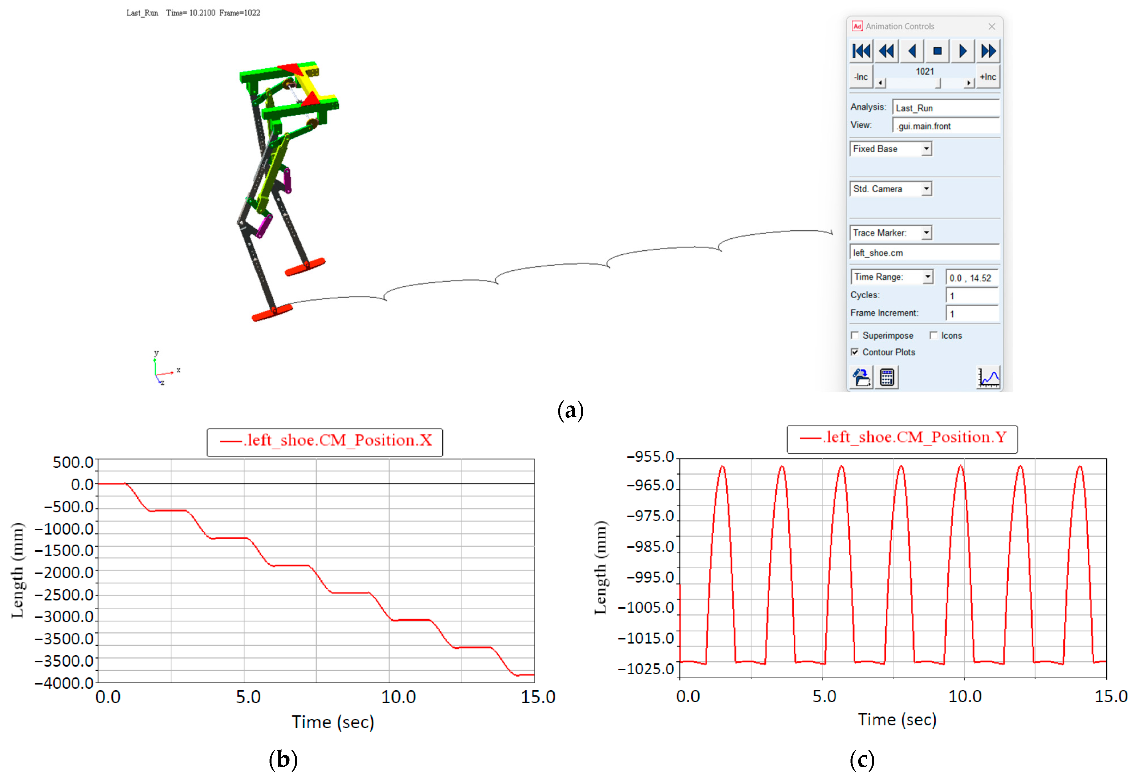
3.4. Kinematic and Dynamic Simulation of the Exoskeleton When Performing Stair Ascent

In order to study the ascent and descent of the stairs in the robotic system, a dynamic simulation was performed under this assumption. For this purpose, an update was performed on the CAD model by replacing the flat support (floor) with a stair model. The contact between the stair and the two exoskeleton soles was defined, keeping the same contact parameters as in the previous case.

The simulation model was built with the help of the multibody dynamic systems analysis software ADAMS View. The development of the dynamic model involved the definition of the kinematic torques, the definition of the materials of the elements and the corresponding definition of the contact between the exoskeleton sole and the stairs. The results obtained are presented below.

A sequence during the exoskeleton motion simulation for staircase motion assistance is shown in Figure 22, when successive frames are presented and where the trajectories described by the two legs are observed.

Another set of results of interest are the laws of variation in the components of the connection forces in the kinematic couplings of the mechanism. These are important for sizing in terms of mechanical strength. Thus, in Figure 23 and Figure 24, these results are shown for the knee and hip joints. Maximum connection force values of 750 N are observed for the knee joint and much higher values for the hip joint.

It should be noted that in the case of the hip joint, a large difference in value occurs between the left and right leg due to the positioning of the drive motor.

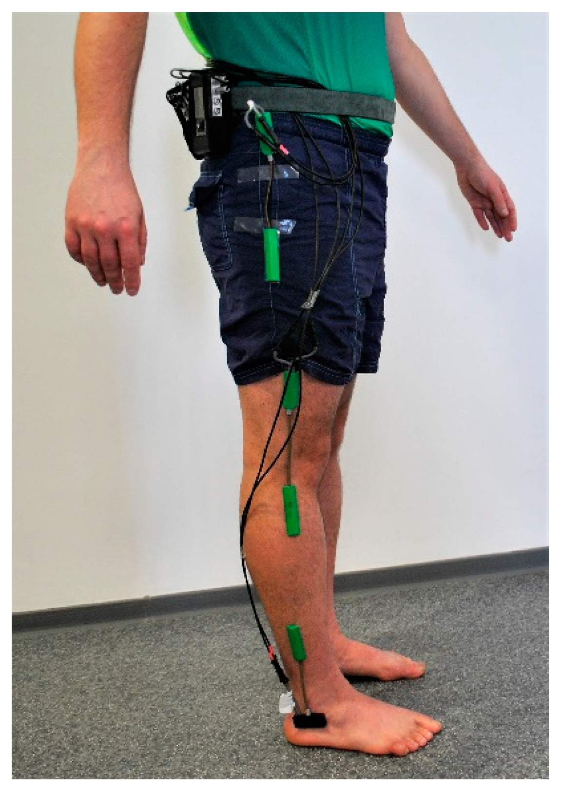
4. Robotic System Fabrication and Experimental Motion Analysis

To manufacture the robotic system, we used 3D printing technology. There are several types of 3D printing; each type has specific characteristics. The most commonly used methods are:

-

Fused deposition modeling (FDM)—This type is the most widely used for 3D printing. By melting a thermoplastic filament and depositing it layer by layer, the model is obtained. The material solidifies as it cools. The filament can be of different diameters, the most commonly used being 1.75 mm. The FDM process is commonly used for prototyping but can also be used for the production of series parts.

-

Stereolithography (SLA)—The process uses liquid resin and a UV laser as material. The UV laser traces the outline of the object after each layer of resin, solidifying the resin to the final part, but it is also toxic.

-

Selective laser sintering (SLS)—This process uses powdered material, most commonly a thermoplastic or metal, that is selectively fused using a high-power laser. The laser heats and melts the powder particles, thereby creating a solid layer. This process is repeated until the part is made. This produces complex, durable parts with no supporting structures during printing.

-

Direct metal laser sintering (DMLS)—DMLS is similar to SLS, but this process specifically uses metal powders. A high-power laser selectively fuses metal powder particles, producing complex metal parts with high strength and durability, used mainly in the aerospace, automotive and medical industries.

When choosing a 3D printing technology, application-specific factors such as part material and complexity, detail and surface quality must be taken into account.

FDM 3D printing offers several benefits that contribute to its popularity and widespread use:

-

Printers using this technology come at affordable prices.

-

They accept a wide range of materials, from thermoplastics to carbon fiber.

-

It is easy to use, with a relatively simple set-up for printing. The slicing software is user-friendly and intuitive. The software is also compatible with standard CAD formats, making it easy to create designs.

-

Reduces material waste compared to traditional technology such as CNC. Waste is minimal as it is an additive manufacturing process, which means that each object is built layer by layer using the minimum amount of material.

-

It is used in research to create prototypes and test concepts but also has an educational role, allowing engineering design principles to be applied in practical applications.

Exoskeleton robotic system parts are printed on a printer using FDM technology on which different types of filaments can be used. Usually, the filaments are thermoplastic materials in the form of a long thread wound on a roll. The material we used is PLA 3D+ (Polylactic Acid). This material is the most commonly used in filaments due to its ease of use, low cost and biodegradable material. It is made from renewable resources such as corn starch or sugar cane. PLA melts at a relatively low temperature, has minimal deformation and can be found in different colors.

Geometrically optimized part designs are manufactured. The CAD file is saved as STL Files (*.stl). This file is imported into 3D Ultimaker Cura (Figure 25). In this program, various parameters can be set, such as model position and model orientation, but also parameters related to the thickness of the deposited layer, the size of the material inside and support. After setting each parameter, by using the “Slice” function, a preview of the simulation of the deposition of the layers by the printhead is made, as well as information about the estimated time of realization, weight and length of filament used. This G-code file is saved on an SD card and inserted into the printer. The printer’s print-bed size of 400×400 mm allowed all components to be printed.

Snapshots during printing for some items are shown in Figure 26.

Through kinematic analysis and dynamic simulation, we validated the feasibility of the virtual prototype of the exoskeleton robotic system. The next step is to build an experimental model and validate it through tests on the real model. Thus, physical models of the component parts were made by additive manufacturing, as shown in Figure 27.

All these parts were assembled according to the exoskeleton design. The kinematic elements that go into the structure of the two legs were assembled by means of 10 mm diameter bolts, as shown in Figure 27. The two legs were assembled on the upper frame. Furthermore, the drive shaft was assembled on this frame, as well as the supports for the vertical support legs of the system (Figure 28). The drive axle is bolted to the upper frame with two supports. The driven wheel of a cylindrical gear with a transmission ratio of 1:2 is attached to this shaft. The drive motor is mounted on the upper frame by means of a screw fastening and is a 24 V Pololu 150:1, 37 D × 57 L, helical pinion, metal electric motor. It is a powerful, 24 V, brushed DC model with a 150:1 metal gearbox. The gearbox consists mainly of gears but has helical gears on the first level for reduced noise and increased efficiency. The motor has a 6 mm diameter, 16 mm long “D” shaped output shaft and the following technical specifications:

Voltage: 24 V; No load performance: 68 RPM, 100 mA; Stall extrapolation: 56 kg⋅cm, 3 A; Size: 37 D × 57 L mm; Weight: 195 g; Shaft diameter: 6 mm; Transmission ratio: 150:1; Speed at maximum efficiency: 59 rpm; Torque at maximum efficiency: 7.3 kg cm.

The exoskeleton was assembled, using bolts to secure the fork elements, as shown in Figure 28.

For experimental motion analysis, we used the ultrafast camera motion analysis method. For this purpose, reflective markers were pasted in the points of interest, and by processing video files, the trajectories of some points of interest, as well as the angular variations in the knee and hip joint, were determined.

During this analysis, the exoskeleton walks on the ground supported by a frame that moves on two support wheels.

Thus, Figure 29 shows aspects of the CONTEMPLAS software, where the angle of variation in the knee and hip joints are determined, as well the determination of the trajectories made by the three leg joints (hip, knee and ankle), as shown in Figure 30.

Apart from the results in the form of snapshots during the Supplementary video, the acquired data are transformed into numerical results. The numerical data are imported into Microsoft Excel, and the graphical results shown below are obtained. In Figure 31, the results in the form of variation laws for the rotation angle in the knee joints are presented. It can be seen that the results obtained experimentally are similar to those obtained by the dynamic simulation, shown in Figure 16a.

The experimentally obtained variation laws for the angles in the exoskeleton hip joints are shown in Figure 32.

As can be seen, the results obtained experimentally for the variation angles in the joints of the experimental prototype are similar to those obtained by numerical simulation.

Another category of results obtained is that represented by the trajectories of some characteristic points, specifically the leg joints. The experimental position during the exoskeleton gait simulation is presented in Figure 33.

The experimental results for the position of the point attached to the ankle joint are similar to those in Figure 15, determined by numerical simulation.

5. Discussion

All three structural solutions shown in Figure 5 achieve an ovoid trajectory of the ankle joint when the mechanical system operates with the upper frame fixed to the base. This is shown in Figure 34, where we have shown the ovoid trajectory obtained by simulating the motion of the solutions in Figure 5b,c. The structural solution in Figure 34b will be reported in future research.

As we have seen in the kinematic study, the structural solution with seven kinematic elements, in Figure 5b, achieves in the knee joint an angular amplitude of 42 deg, lower than in the normal gait where we have 55 deg. This fact does not prevent its use for rehabilitation, as it is a viable solution for implementation in exoskeleton systems, since, in some cases, it is recommended that the rehabilitation of patients with locomotor disabilities be performed with smaller angular amplitudes than in a normal gait.

To validate the numerical simulation results, we have shown, in Figure 35, a comparative analysis between flexion–extension angles in the knee and hip joints obtained by two methods: experimental and simulation. In Figure 35a, we have shown the comparison of the experimental and simulation angles for the knee joint. Since, in the numerical simulation, we determined the angle between the two elements forming the knee joint, we used the same way of measuring the angle from the experimental data. In this way, the variation is between the range 138–176 deg. For the comparison between the measured and simulated values for the angle in the hip joint, shown in Figure 35b, we used the value of the rotation angle in the joint, so the variation starts from zero. It can be seen that there are differences in the overlap of the two curves, and this comes from the different speeds of the drive motors for the simulation and experiment. For the simulation, we used a found speed of 1.5 rad/s for the actuator, and in the experimental model, the actuator angular velocity shows variations due to the variation in the electric motor load. However, there is an agreement between the two categories of results, so we can conclude that both categories of results are valid.

Another category of results obtained by numerical simulation are the connecting forces in the knee and hip joints. Here we can make a comparison between the results obtained in two exoskeleton simulation situations: walking the exoskeleton on a flat surface and climbing stairs. It can be seen from the analysis of Figure 23 that when climbing up a staircase, the values of the components along the X-axis of the connection force increase, while the components along the Y-axis decrease.

As further research directions, we propose the theoretical and experimental study of the solution for Figure 5c, which has nine kinematic elements in its structure.

6. Conclusions

In this research, a new exoskeleton design solution is studied. Two structural solutions are proposed for analysis, the first with seven kinematic elements in the structure and the second with nine kinematic elements in the structure. Both solutions are driven by a single motor element and realize ovoid shoe trajectories. In this paper, we have studied the solution with seven kinematic elements. For this solution we designed a structurally optimized virtual model. We have developed an experimental prototype that is manufactured by additive manufacturing. To study the motion of this prototype, we used motion analysis based on a high-speed video camera system. The experimental results validate the numerical simulation models in ADAMS. Moreover, the motion simulation is performed in two scenarios: walking on a flat surface and walking on an inclined plane. Therefore, another future research direction is to study the possibility of assisting stair walking with this exoskeleton solution. Moreover, in the future research, we aim to study by numerical simulation the dynamics of the exoskeleton, considering the friction in the kinematic couplings in the situation when the exoskeleton is used by a virtual dummy.

In conclusion, the aim of this research is to develop an exoskeleton-type robotic system based on the implementation in the foot structure of a mono-mobile kinematic chain that includes in its structure the kinematic couplings of the human foot (i.e., hip and knee) and that performs movements similar to human walking.

References

1. Malyuga, O.O. The Design of the Exoskeleton; IPR-Media: Saratov, Russia, 2019. [Google Scholar]
2. Yagn, N. Apparatus for Facilitating Walking, Running and Jumping. U.S. Patent No. 420,179, 28 January 1890. [Google Scholar]
3. Mizen, N.J. Powered Exoskeletal Apparatus for Amplifying Human Strength in Response to Normal Body Movements. Patent No. 3449769, 17 June 1969. [Google Scholar]
4. Shi, D.; Zhang, W.; Zhang, W.; Ding, X. A review on lower limb rehabilitation exoskeleton robots. Chin. J. Mech. Eng. 2019, 32, 74. [Google Scholar] [CrossRef]
5. Chaichaowarat, R.; Prakthong, S.; Thitipankul, S. Transformable Wheelchair–Exoskeleton Hybrid Robot for Assisting Human Locomotion. Robotics 2023, 12, 16. [Google Scholar] [CrossRef]
6. Hu, B.; Liu, F.; Cheng, K.; Chen, W.; Shan, X.; Yu, H. Stiffness optimal modulation of a variable stiffness energy storage hip exoskeleton and experiments on its assistance effect. IEEE Trans. Neural Syst. Rehabil. Eng. 2023, 31, 1045–1055. [Google Scholar] [CrossRef] [PubMed]
7. Carbone, G.; Laribi, M.A. Recent trends on innovative robot designs and approaches. Appl. Sci. 2023, 13, 1388. [Google Scholar] [CrossRef]
8. Rodrigues-Carvalho, C.; Fernández-García, M.; Pinto-Fernández, D.; Sanz-Morere, C.; Barroso, F.O.; Borromeo, S.; Del-Ama, A.J. Benchmarking the effects on human–exoskeleton interaction of trajectory, admittance and EMG-triggered exoskeleton movement control. Sensors 2023, 23, 791. [Google Scholar] [CrossRef]
9. Jayaraman, C.; Embry, K.R.; Mummidisetty, C.K.; Moon, Y.; Giffhorn, M.; Prokup, S.; Jayaraman, A. Modular hip exoskeleton improves walking function and reduces sedentary time in community-dwelling older adults. J. Neuroeng. Rehabil. 2022, 19, 144. [Google Scholar] [CrossRef]
10. Arcos-Legarda, J.; Torres, D.; Velez, F.; Rodríguez, H.; Parra, A.; Gutiérrez, Á. Mechatronics Design of a Gait-Assistance Exoskeleton for Therapy of Children with Duchenne Muscular Dystrophy. Appl. Sci. 2023, 13, 839. [Google Scholar] [CrossRef]
11. Veneman, J.F.; Kruidhof, R.; Hekman, E.E.; Ekkelenkamp, R.; Van Asseldonk, E.H.; Van Der Kooij, H. Design and evaluation of the LOPES exoskeleton robot for interactive gait rehabilitation. IEEE Trans. Neural Syst. Rehabil. Eng. 2007, 15, 379–386. [Google Scholar] [CrossRef]
12. Huo, W.; Mohammed, S.; Moreno, J.C.; Amirat, Y. Lower limb wearable robots for assistance and rehabilitation: A state of the art. IEEE Syst. J. 2014, 10, 1068–1081. [Google Scholar] [CrossRef]
13. Zhou, J.; Yang, S.; Xue, Q. Lower limb rehabilitation exoskeleton robot: A review. Adv. Mech. Eng. 2021, 13, 16878140211011862. [Google Scholar] [CrossRef]
14. Lee, H.; Ferguson, P.W.; Rosen, J. Chapter 11—Lower Limb Exoskeleton Systems Overview; Rosen, J., Ferguson, P.W., Robotics, W., Eds.; Academic Press: Cambridge, MA, USA, 2020; pp. 207–229. ISBN 9780128146590. [Google Scholar] [CrossRef]
15. Parra-Dominguez, G.S.; Taati, B.; Mihailidis, A. 3D human motion analysis to detect abnormal events on stairs. In Proceedings of the 2012 Second International Conference on 3D Imaging, Modeling, Processing, Visualization & Transmission, Zurich, Switzerland,, 13–15 October 2012; pp. 97–103. [Google Scholar]
16. Ko, C.Y.; Ko, J.; Kim, H.J.; Lim, D. New wearable exoskeleton for gait rehabilitation assistance integrated with mobility system. Int. J. Precis. Eng. Manuf. 2016, 17, 957–964. [Google Scholar] [CrossRef]
17. Chen, B. Recent developments and challenges of lower extremity exoskeletons. J. Orthop. Transl. 2016, 5, 26–37. [Google Scholar] [CrossRef]
18. Anama, K.; Al-Jumaily, A.A. Active exoskeleton control systems: State of the art. Procedia Eng. 2012, 41, 988–994. [Google Scholar] [CrossRef]
19. Díaz, I.; Gil, J.J.; Sánchez, E. Lower-limb robotic rehabilitation: Literature review and challenges. J. Robot. 2011, 2011, 759764. [Google Scholar] [CrossRef]
20. Devi, M.G.; Amutheesan, M.; Govindhan, R.; Karthikeyan, B. A review of three-dimensional printing for biomedical and tissue engineering applications. Open Biotechnol. J. 2018, 12, 241–255. [Google Scholar] [CrossRef]
21. Li, Z.; Deng, C.; Zhao, K. Human-cooperative control of a wearable walking exoskeleton for enhancing climbing stair activities. IEEE Trans. Ind. Electron. 2019, 67, 3086–3095. [Google Scholar] [CrossRef]
22. Woo, H.; Kong, K.; Rha, D.W. Lower-limb-assisting robotic exoskeleton reduces energy consumption in healthy young persons during stair climbing. Appl. Bionics Biomech. 2021, 2021, 8833461. [Google Scholar] [CrossRef] [PubMed]
23. Chandrapal, M.; Chen, X.; Wang, W. Preliminary evaluation of a lower-limb exoskeleton-stair climbing. In Proceedings of the 2013 IEEE/ASME International Conference on Advanced Intelligent Mechatronics, Wollongong, Australia, 9–12 July 2013; pp. 1458–1463. [Google Scholar]
24. Borooghani, D.; Hadi, A.; Alipour, K. Falling Analysis and Examination of Different Novel Strategies for Preserving the Postural Stability of a User Wearing ASR-EXO during Stair Climbing. J. Intell. Robot. Syst. 2022, 105, 5. [Google Scholar] [CrossRef]
25. Xu, F.; Lin, X.; Cheng, H.; Huang, R.; Chen, Q. Adaptive stair-ascending and stair-descending strategies for powered lower limb exoskeleton. In Proceedings of the 2017 IEEE International Conference on Mechatronics and Automation (ICMA), Takamatsu, Japan, 6–9 August 2017; pp. 1579–1584. [Google Scholar]
26. Li, Z.; Yuan, Y.; Luo, L.; Su, W.; Zhao, K.; Xu, C.; Pi, M. Hybrid brain/muscle signals powered wearable walking exoskeleton enhancing motor ability in climbing stairs activity. IEEE Trans. Med. Robot. Bionics 2019, 1, 218–227. [Google Scholar] [CrossRef]
27. Zhang, Z.; Zhu, Y.; Zheng, T.; Zhao, S.; Ma, S.; Fan, J.; Zhao, J. Lower extremity exoskeleton for stair climbing augmentation. In Proceedings of the 2018 3rd International Conference on Advanced Robotics and Mechatronics (ICARM), Singapore, 18–20 July 2018; pp. 762–768. [Google Scholar]
28. Baltrusch, S.J.; Van Dieën, J.H.; Van Bennekom, C.A.M.; Houdijk, H. The effect of a passive trunk exoskeleton on functional performance in healthy individuals. Appl. Ergon. 2018, 72, 94–106. [Google Scholar] [CrossRef]
29. Ishmael, M.K.; Archangeli, D.; Lenzi, T. A powered hip exoskeleton with high torque density for walking, running, and stair ascent. IEEE/ASME Trans. Mechatron. 2022, 27, 4561–4572. [Google Scholar] [CrossRef]
30. Zhang, Z.W.; Liu, G.F.; Zheng, T.J.; Li, H.W.; Zhao, S.K.; Zhao, J.; Zhu, Y.H. Blending control method of lower limb exoskeleton toward tripping-free stair climbing. ISA Trans. 2022, 131, 610–627. [Google Scholar] [CrossRef]
31. Bae, E.; Park, S.E.; Moon, Y.; Chun, I.T.; Chun, M.H.; Choi, J. A robotic gait training system with stair-climbing mode based on a unique exoskeleton structure with active foot plates. Int. J. Control Autom. Syst. 2020, 18, 196–205. [Google Scholar] [CrossRef]
32. Böhme, M.; Köhler, H.P.; Thiel, R.; Jäkel, J.; Zentner, J.; Witt, M. Preliminary Biomechanical Evaluation of a Novel Exoskeleton Robotic System to Assist Stair Climbing. Appl. Sci. 2022, 12, 8835. [Google Scholar] [CrossRef]
33. Joudzadeh, P.; Hadi, A.; Alipour, K.; Tarvirdizadeh, B. Design and implementation of a cable driven lower limb exoskeleton for stair climbing. In Proceedings of the 2017 5th RSI International Conference on Robotics and Mechatronics (ICRoM), Tehran, Iran, 25–27 October 2017; pp. 76–81. [Google Scholar]
34. Jang, J.; Kim, K.; Lee, J.; Lim, B.; Shim, Y. Assistance strategy for stair ascent with a robotic hip exoskeleton. In Proceedings of the 2016 IEEE/RSJ International Conference on Intelligent Robots and Systems (IROS), Daejeon, Korea, 9–14 October 2016; pp. 5658–5663. [Google Scholar]
35. Geonea, I.; Dumitru, S.; Copilusi, C.; Margine, A.; Rinderu, P. Design and numerical characterization of a leg exoskeleton linkage for motion assistance. In Proceedings of the 2018 World Congress on Engineering and Computer Science, San Francisco, CA, USA, 23–25 October 2018; pp. 23–25. [Google Scholar]
36. Geonea, I.; Copilusi, C.; Margine, A.; Dumitru, S.; Rosca, A.; Tarnita, D. Dynamic Analysis and Structural Optimization of a New Exoskeleton Prototype for Lower Limb Rehabilitation. In New Trends in Medical and Service Robotics; Tarnita, D., Dumitru, N., Pisla, D., Carbone, G., Geonea, I., Eds.; Springer: Cham, Switzerland, 2023; Volume 133. [Google Scholar] [CrossRef]
37. Geonea, I.; Dumitru, N.; Ceccarelli, M.; Tarnita, D. Kinematic and Dynamic Analysis of a New Mechanism for Assisting Human Locomotion. In New Trends in Medical and Service Robotics; Tarnita, D., Dumitru, N., Pisla, D., Carbone, G., Geonea, I., Eds.; Springer: Cham, Switzerland, 2023; Volume 133. [Google Scholar] [CrossRef]
Figure 1. Human subject on which goniometer sensors are mounted.
Machines 11 01000 g001
Figure 2. Acquired ankle-joint angles during human walking: (a) right ankle joint; (b) left ankle joint.
Machines 11 01000 g002
Figure 3. Acquired knee-joint angles during human walking: (a) right knee joint; (b) left knee joint.
Machines 11 01000 g003
Figure 4. Acquired hip-joint angles during human walking: (a) right hip joint; (b) left hip joint.
Machines 11 01000 g004
Figure 5. Structural solutions for the kinematic chain of an exoskeleton leg: (a) first solution with 7 links; (b) second solution with 7 links; (c) third solution with 9 links.
Machines 11 01000 g005
Figure 6. Scheme for the kinematic computation of the foot mechanism.
Machines 11 01000 g006
Figure 7. The mechanism Assur groups.
Machines 11 01000 g007
Figure 8. Block diagram of the structural optimization process.
Machines 11 01000 g008
Figure 9. Specification of geometrical parameters defined as design variables.
Machines 11 01000 g009
Figure 10. Response chart for the output parameter total deformation maximum: (a) versus input parameters P11 and P12; (b) versus input parameters P12 and P13.
Machines 11 01000 g010
Figure 11. Response chart for the output parameter solid mass: (a) versus input parameters P11 and P12; (b) versus input parameters P12 and P13.
Machines 11 01000 g011
Figure 12. Response chart for the output parameter equivalent stress maximum: (a) versus input parameters P11 and P12; (b) versus input parameters P12 and P13.
Machines 11 01000 g012
Figure 13. Maps with the total deformation and equivalent stress distribution for the optimal geometric shape: (a) total deformation; (b) equivalent (von-Mises) stress.
Machines 11 01000 g013
Figure 14. Structurally optimized CAD model of the exoskeleton system.
Machines 11 01000 g014
Figure 15. Kinematic simulation of the exoskeleton: (a) the path performed by point K, corresponding to the ankle joint; (b) point K ovoid trajectory, computed in XY coordinates.
Machines 11 01000 g015
Figure 16. Computed exoskeleton joint angle variation: (a) for the knee joint; (b) for the hip joint.
Machines 11 01000 g016
Figure 17. The exoskeleton simulation while walking on the floor: (a) the trajectory computed during the exoskeleton gait simulation; (b) the law of variation in the X coordinate of point K; (c) the law of variation in the Y coordinate of point K.
Machines 11 01000 g017
Figure 18. Exoskeleton walking simulation successive frames.
Machines 11 01000 g018
Figure 19. Laws of variation in connection forces in the exoskeleton knee joint: (a) left knee joint Fx; (b) left knee joint Fy; (c) right knee joint Fx; (d) right knee joint Fy.
Machines 11 01000 g019
Figure 20. Laws of variation in connection forces in the exoskeleton hip joint: (a) left hip joint Fx; (b) left hip joint Fy; (c) right hip joint Fx; (d) right hip joint Fy.
Machines 11 01000 g020
Figure 21. Computed motor torque variation.
Machines 11 01000 g021
Figure 22. The trajectory described by the sole while climbing the stairs and exoskeleton snapshots from climbing the stairs.
Machines 11 01000 g022
Figure 23. Laws of variation in connection forces in the exoskeleton knee joint when it is performing stair ascent: (a) left knee joint Fx; (b) left knee joint Fy; (c) right knee joint Fx; (d) right knee joint Fy.
Machines 11 01000 g023
Figure 24. Laws of variation in connection forces in the exoskeleton hip joint: (a) left hip joint; (b) right hip joint.
Machines 11 01000 g024
Figure 25. G-Code file generation in Ultimaker Cura.
Machines 11 01000 g025
Figure 26. Exoskeleton parts 3D printing.
Machines 11 01000 g026
Figure 27. Assembly of the exoskeleton legs to the upper frame.
Machines 11 01000 g027
Figure 28. Assembled model of the exoskeleton robotic system.
Machines 11 01000 g028
Figure 29. Determination of joint variation angles using CONTEMPLAS software: (a) hip joint angle tracking; (b) knee joint angle tracking.
Machines 11 01000 g029
Figure 30. Determination of foot joint trajectories using CONTEMPLAS software: (a) beginning of the exoskeleton motion; (b) ending of the exoskeleton motion.
Machines 11 01000 g030
Figure 31. The laws of angle variation for knee joints of the exoskeleton leg: (a) right knee angle; (b) left knee angle.
Machines 11 01000 g031
Figure 32. The laws of variation in hip-joint angles for the exoskeleton: (a) right hip angle; (b) left hip angle.
Machines 11 01000 g032
Figure 33. The experimental position during the exoskeleton gait simulation: (a) the law of variation in the X coordinate of point M, attached to the sole of the exoskeleton foot; (b) the law of variation in the Y coordinate of point M, attached to the sole of the exoskeleton foot.
Machines 11 01000 g033
Figure 34. The ovoid trajectory described by the trailing point of the exoskeleton leg mechanism: (a) structural solution with 7 kinematic elements; (b) structural solution with 9 kinematic elements.
Machines 11 01000 g034
Figure 35. Comparison of experimentally measured and simulated exoskeleton flexion/extension angles: (a) for the knee joint; (b) for the hip joint.
Machines 11 01000 g035