A Guiding and Positioning Motion Strategy Based on a New Conical Virtual Fixture for Robot-Assisted Oral Surgery

Abstract

In robot-assisted oral surgery, the surgical tool needs to be fed into the target position to perform surgery. However, unmodeled extraoral and complex intraoral environments bring difficulties to motion planning. Meanwhile, the motion is operated manually by the surgeon, causing relatively limited accuracy as well as the risk of misoperation. Moreover, the random movements of the patient’s head bring additional disturbance to the task. To achieve the task, a motion strategy based on a new conical virtual fixture (VF) was proposed. First, by preoperatively specifying a conical guiding cone as the VF, virtual repulsive forces were applied on the out-of-range end effector. Then, based on the two-point adjustment model and velocity conversion, the effect of VF was established to prevent the end-effector from exceeding the constraint region. Finally, a vision system corrects the guiding cone to compensate for the random movement of the patient’s head to feed to a dynamic target. As an auxiliary framework for surgical operation, the proposed strategy has the advantages of safety, accuracy, and dynamic adaptability. Both simulations and experiments are conducted, verifying the feasibility of the proposed strategy.

1. Introduction

1.1. Background and Task

Oral diseases, such as oral tumors and tooth loss, are very common worldwide [1,2,3], and reduce the life quality of patients [4,5]. Oral surgery, such as tumor resection and dental implant, is indispensable in the treatment of oral diseases [6,7]. Traditional oral surgery relies entirely on the manual operation of the surgeon, so the accuracy, safety, and prognosis quality cannot be well guaranteed. The development of robotics provides new ways for oral surgery, which has great potential to assist surgeons to provide high-quality surgery and become the mainstream solution in the future [8,9,10].

This paper focuses on a new oral surgery robot system (OSRS) that is under development [11,12,13]. To perform the surgery, it is an important step to feed the end-effector from an arbitrary initial position outside the mouth into the target position inside the oral cavity, which is also the research objective of this paper.

This task is similar to the motion planning of industrial manipulators moving from a start position to the destination, and there are two typical methods: heuristic algorithm [14] and optimization-based algorithm [15]. However, as for the OSRS, unmodeled extraoral environment, complex oral geometry, and dynamic target are three features that bring additional difficulties. First, the extraoral environment is unstructured, which means obstacles like operating tables are not modeled in advance, making it difficult to deploy automatic planning due to the lack of collision detection. Second, the oral cavity is similar to the lofting surface with a complicated structure [16], which is adverse to the real-time performance of collision detection and automatic planning. Third, patients in oral surgery are usually not under general anesthesia, thus there are random disturbance movements in the head, making the oral cavity dynamic rather than static, which requires real-time trajectory generation. In addition, the surgical tool is usually a rigid rod, forming a geometric configuration in which a rigid rod (end effector) is inserted into the oral cavity through the mouth. This configuration makes the end effector surrounded by the inner surfaces of the oral cavity, rather than a typical bounding box such as a cuboid, sphere, or cylinder [17]. This condition limits the adjustment space of the end-effector and reduces the fault tolerance. To sum up, the feeding task is more complex, and an effective strategy needs to be designed to achieve safe and accurate guiding and positioning.

1.2. Related Work

In recent years, oral surgical robots have been studied by scholars. On the one hand, computer vision is widely used. Ma et al. [18] proposed a markerless model to execute preoperative planning for the maxillofacial surgery robot. Hu et al. [19] used deep learning to detect the oral cavity and generated the trajectory for a transoral robot by using oral center constraint and optimization methods. Cheng et al. [20] obtained the implantation point through an L-shaped intraoral marker, and its transformation is derived to achieve accurate positioning. Toosi et al. [21] developed simulation software for a master–slave dental robot using collision detection. On the other hand, master–slave control and cooperative control are commonly adopted. Kasahara et al. [22] achieved better dental drilling through the hybrid force/position control strategy in the master–slave control for dental drilling robot, and Iijima et al. [23] also adopted a similar control strategy in their work. Li et al. [24] used motion mapping with position and pose separated and converted the pose increments by the rotation vector method. Kwon et al. [25] developed a master–slave transoral robot system. The above works have studied the navigation and motion control of oral surgical robots, where master–slave control and computer vision are mostly adopted, and meaningful contributions are made.

Besides, as a key means for guidance and safety, virtual fixture (VF) plays an important role in surgical robots and has attracted many scholars. Rosenberg proposed the concept of VF for teleoperation [26]. Abbott et al. [27,28] and Bettini et al. [29] proposed different types of VF, and admittance control was combined [30]. Kikuuwe et al. [31] proposed a plastic VF that can either guide the operation or force it to escape from the VF. These works have built the foundation of VF, which is widely used in medical robots [32,33]. Subsequently, some scholars have done more research on VF. Tang et al. [34] simplified the organs from a group of points, and then established the VF through collision detection, artificial potential fields, and force feedback, to achieve safe master–slave operation. Pruks et al. [35] used an RGB-D camera to generate the VF in unstructured environments. Similarly, Marinho et al. [36] constructed the VF using vector field inequalities through a set of points. Xu et al. [37] and Li et al. [38] designed virtual fixtures for orthopedic surgery and nasal surgery respectively using 3D models and geometric algorithms. Ren et al. [39] trained a neural network to fit the geometry of the heart to build a virtual fixture. He et al. [40] established VF for an ophthalmic robot by converting the contact force to the velocity of the probe. The above research enrich the theory and application of VF and are very constructive to the work of this paper.

However, prior studies rarely involved VF to better adapt to oral surgery. Additionally, most VF focus only on position control, while orientation is less involved, lowering the fault tolerance under the geometric configuration of oral surgery. In general, motion strategies for oral surgery robots are still limited, and a convenient and integrated solution is still needed. Thus, this paper proposes a guiding and positioning strategy for the OSRS. In the strategy, a flared guiding cone is designed as the VF to better fit the oral structure after the master–slave control is built. Subsequently, the two-point adjustment model and velocity conversion are derived as the effect of the VF to adjust the surgical tool. Next, the VF is integrated with the vision system to compensate for the head disturbance of the patient, becoming the full strategy proposed. In addition, the strategy also provides an optional, automatic mode that differs from typical automatic planning methods. The main contributions of this paper can be summarized as follows:

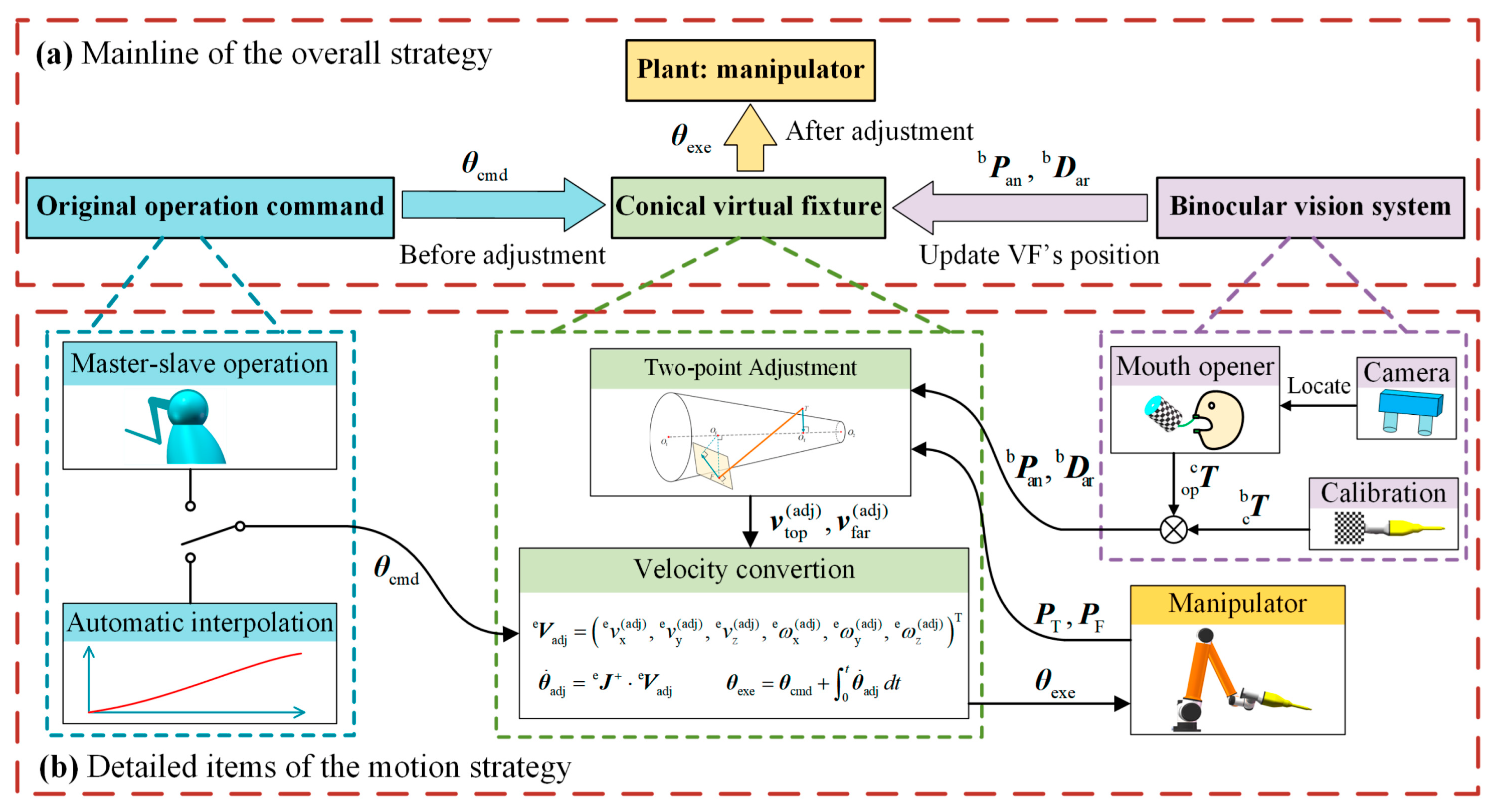
• A new conical virtual fixture is proposed for surgical operation with the master–slave mapping built. In the virtual fixture, a flared guiding cone is designed in accordance with the geometric configuration of oral surgery.
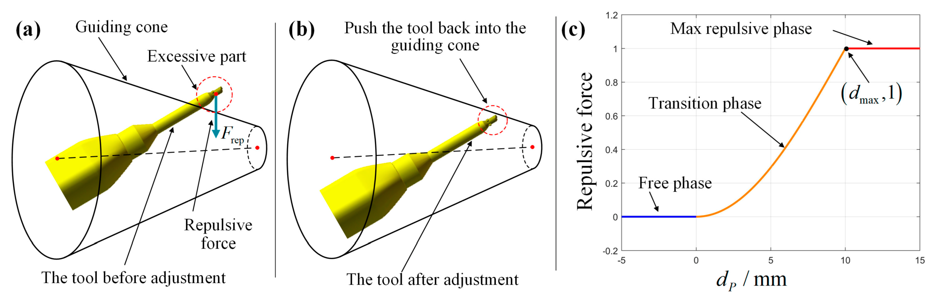
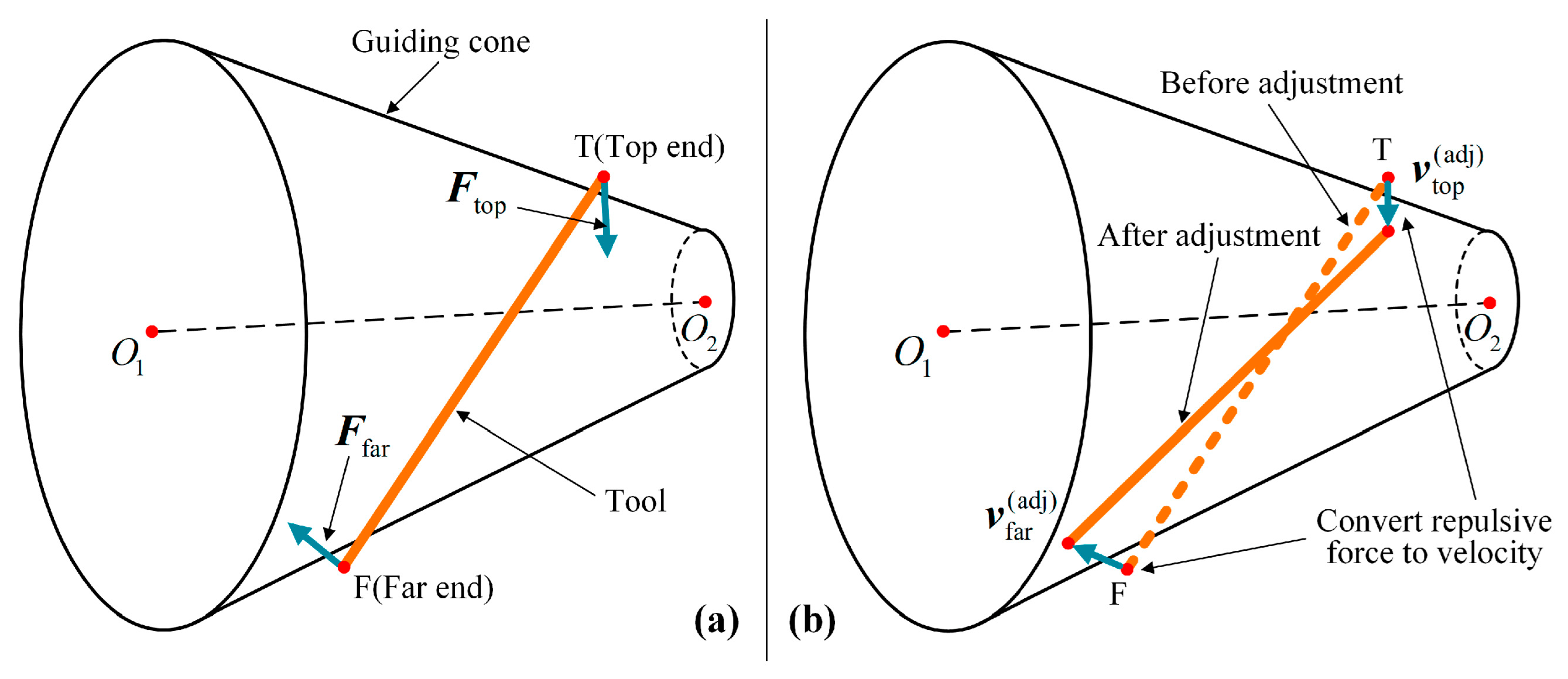
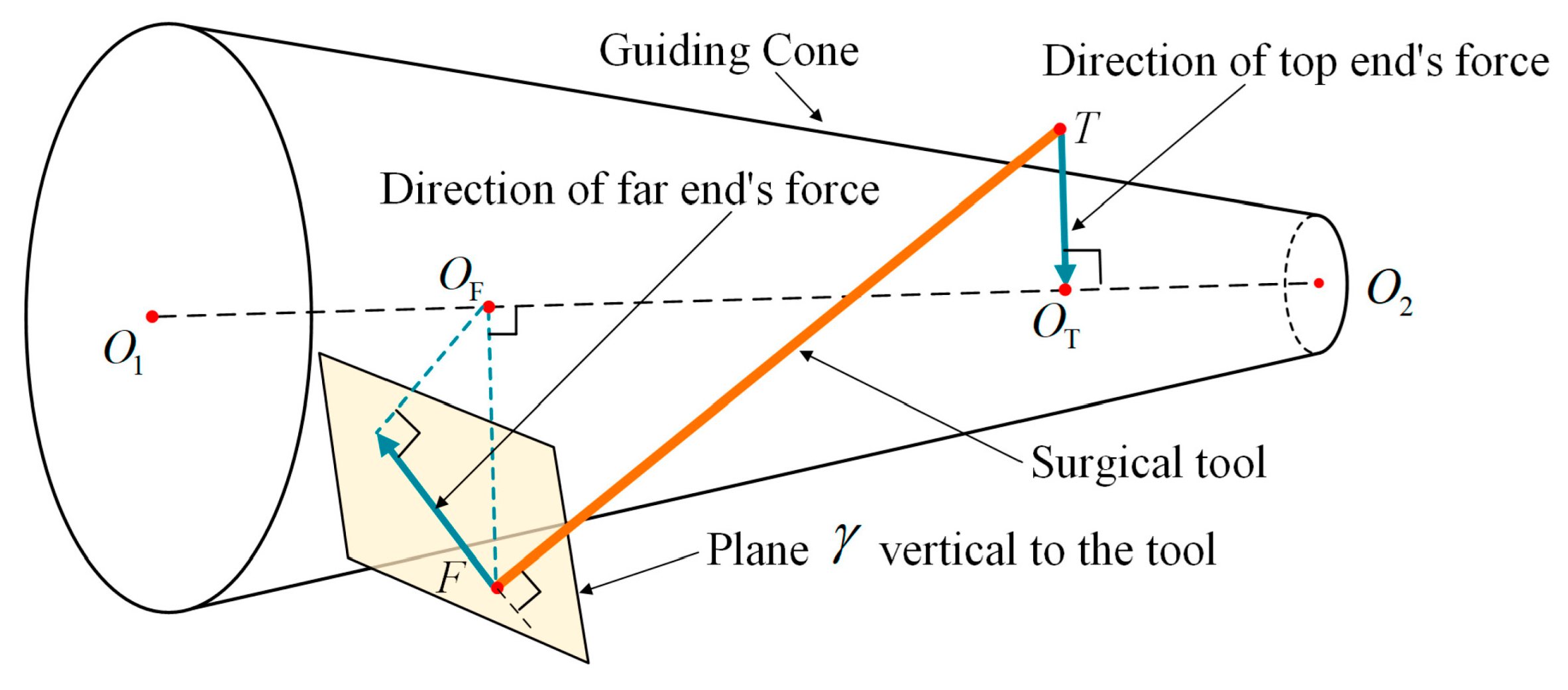
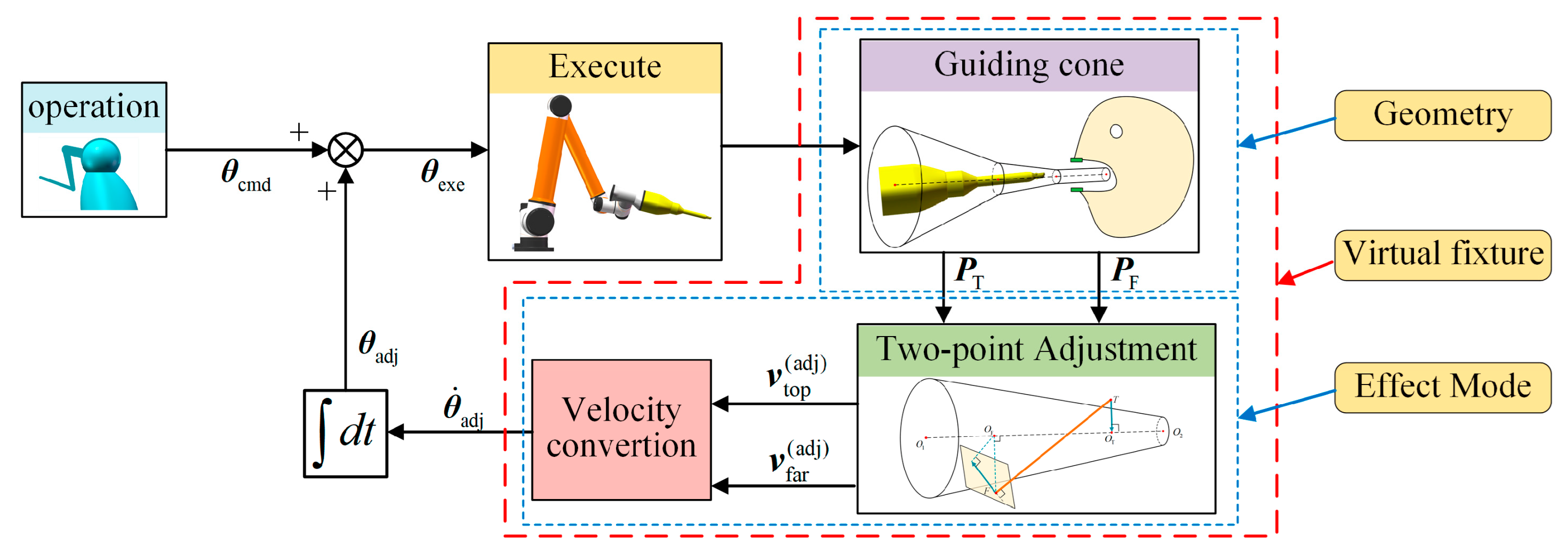
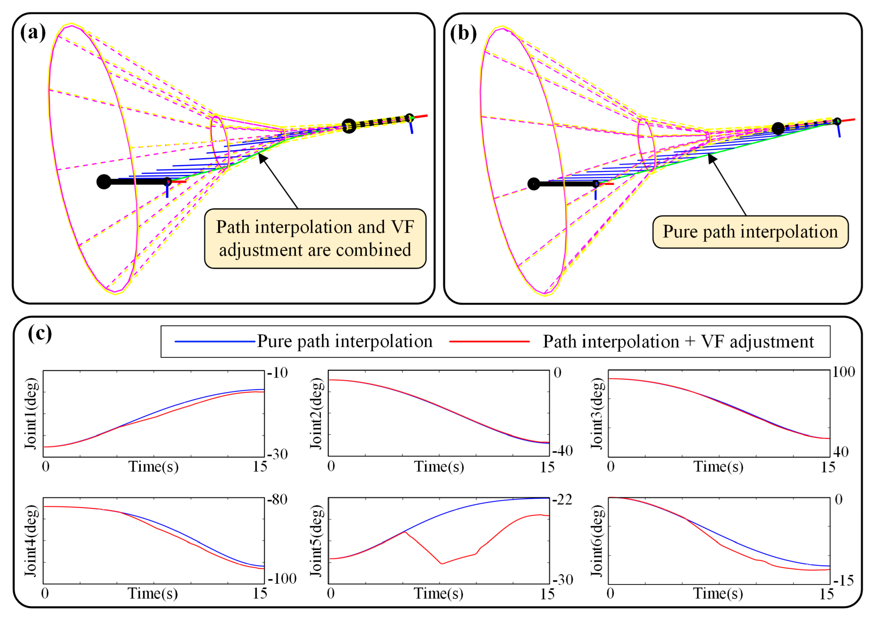
• Two-point adjustment model and velocity conversion are proposed to be the effect of the VF, which can simultaneously adjust the position and orientation of the tool.
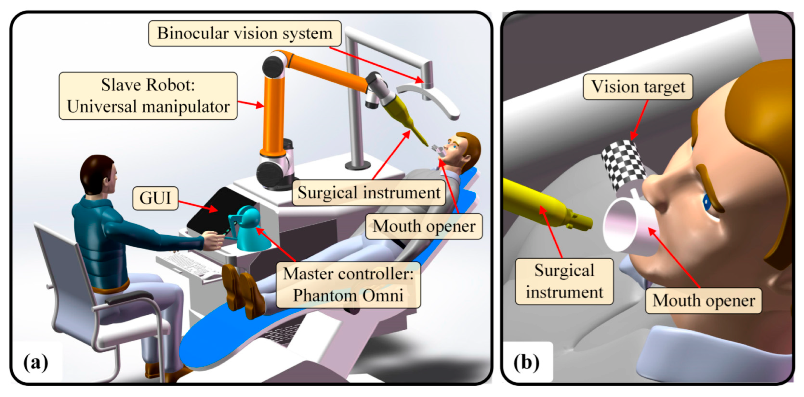
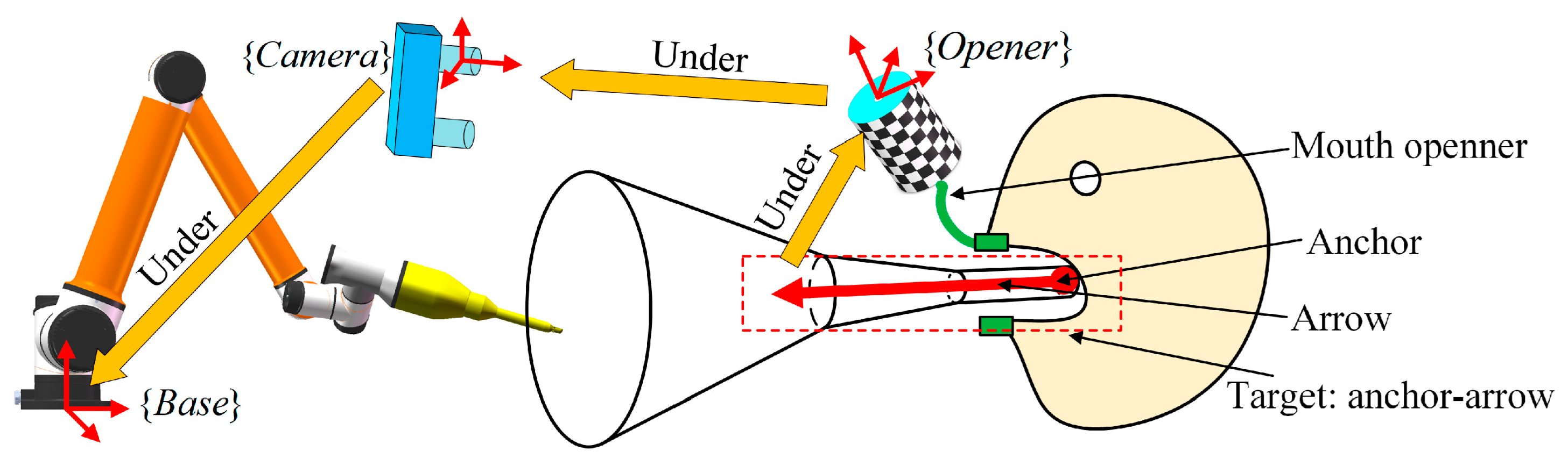
• A new mouth opener is used as a marker for the vision system to locate the oral cavity. The guiding cone is corrected in real-time to compensate for the random disturbance of the patient’s head and realize the feeding to the dynamic target.
• The new VF and vision system are integrated into a full guiding and positioning strategy. This strategy serves as a novel active adjustment framework that not only assists safe and accurate feeding, but also provides an automatic mode to choose.

The rest of this paper is organized as follows. Section 2 presents the OSRS, where hardware constitution and master–slave mapping are given. Section 3 introduces the concept of the conical virtual fixture. Section 4 describes the effect of the guiding cone, including the two-point adjustment model and velocity conversion, and hence the new VF is fully designed. Section 5 introduces system integration, especially the combination of a binocular vision system. Simulations and experimental validations are given in Section 6. Finally, conclusions are drawn in Section 7.

2. Oral Surgery Robot System (OSRS)

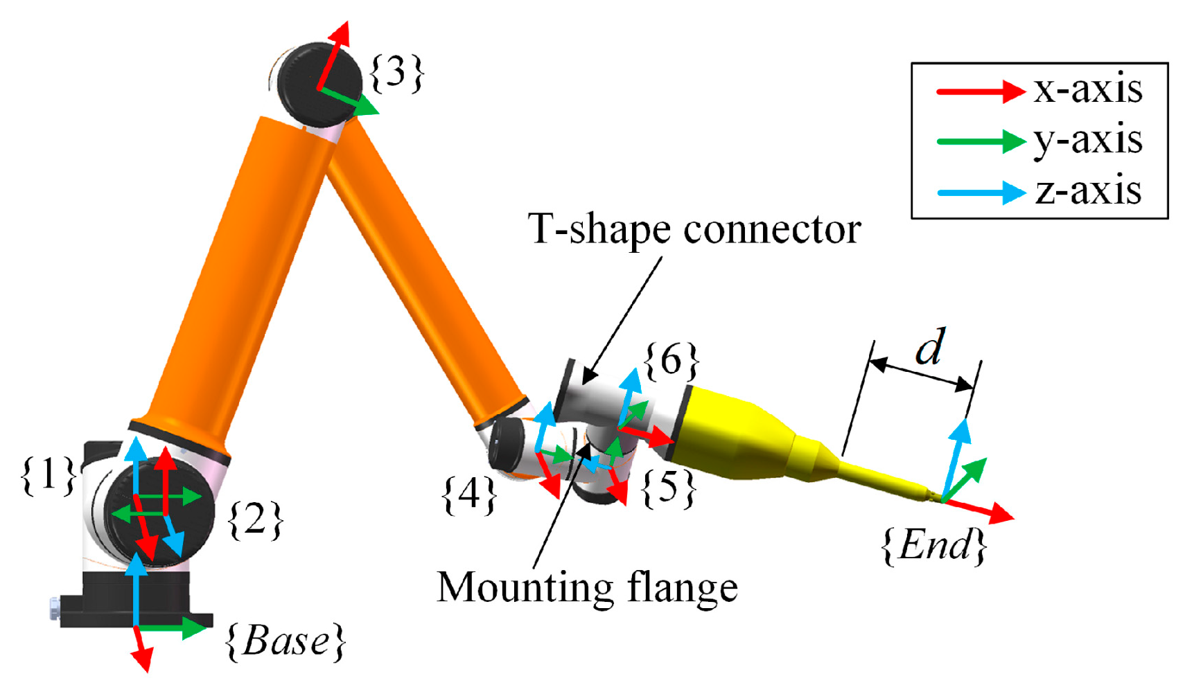
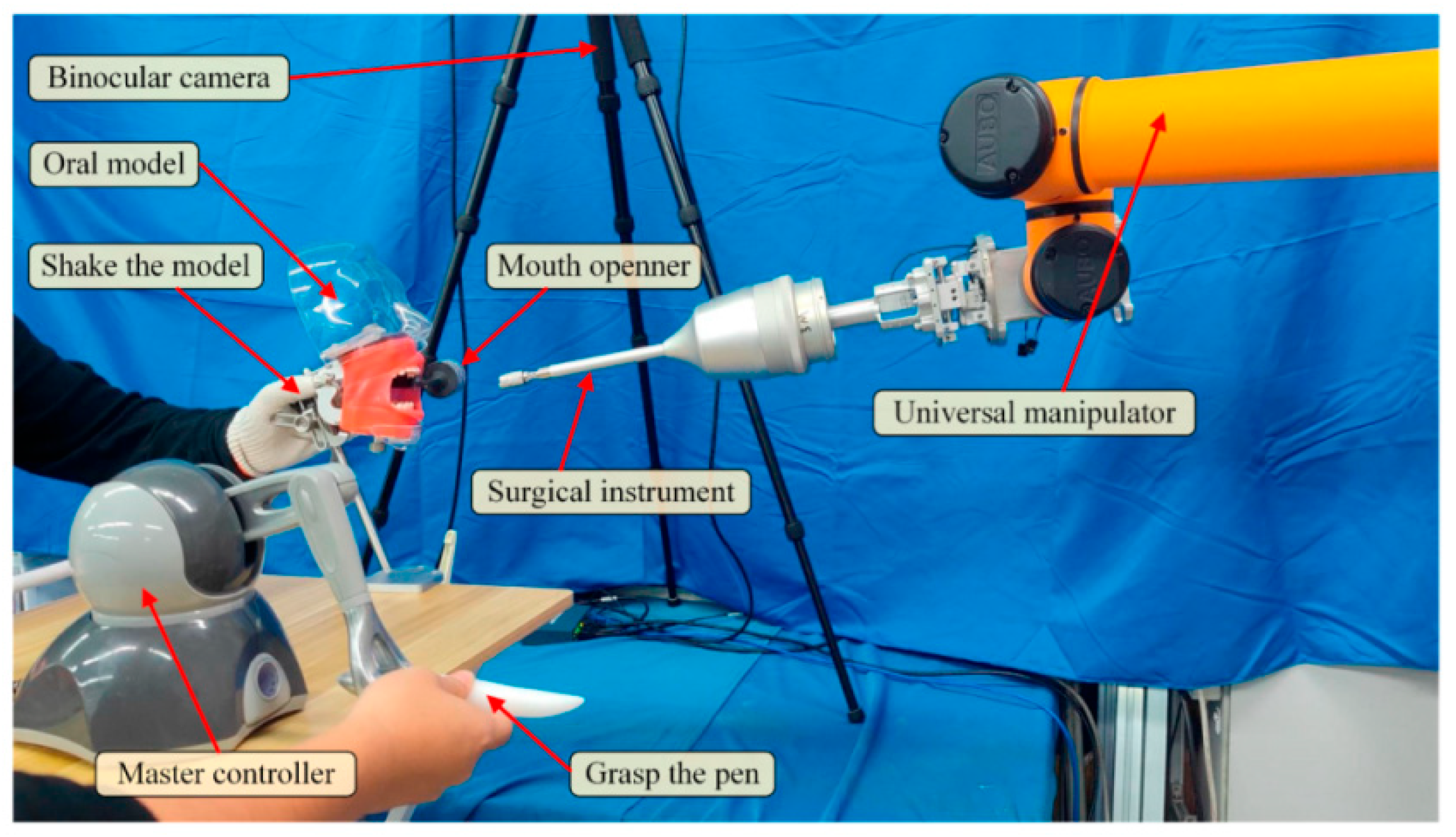
2.1. Hardware Constitution

The hardware of OSRS includes a universal manipulator, a surgical instrument, a master controller, a mouth opener, and a vision system. The universal manipulator has 6 DOFs, with the surgical instrument mounted on it. Surgical instruments, also the end effector, have four types: wound suture, dental implant, laser drilling, and tumor resection. The master controller is a Phantom Omni product, by which the surgeon can drive the manipulator and take the surgical instrument into the oral cavity. The mouth opener can expand the patient’s mouth while serving as a marker for vision localization. The vision system can locate the oral cavity when the mouth opener is detected. The OSRS is shown in Figure 1a, and the mouth opener is shown in Figure 1b.

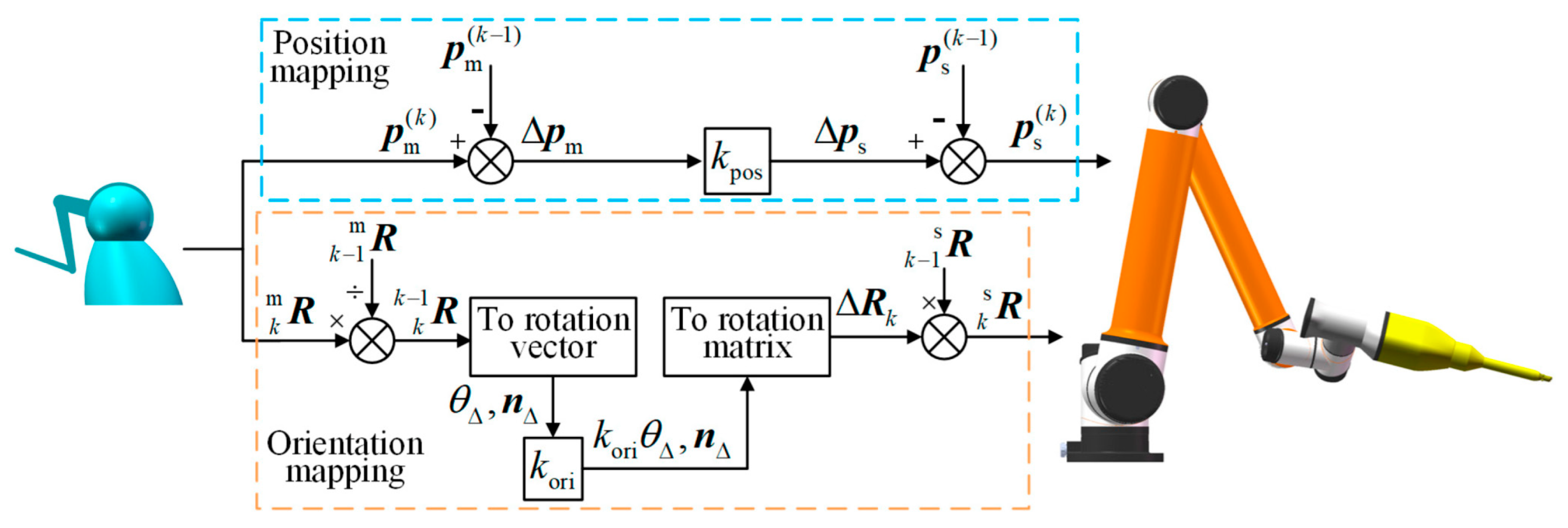
2.2. Master–Slave Mapping

The master–slave mapping of the OSRS includes position mapping and orientation mapping. The position and orientation of the master controller can be obtained from the phantom’s API. Both position mapping and orientation mapping are incremental, which means the master controller’s increment is mapped to the slave manipulator by a scaling factor. For position, the mapping is shown in Equation (1).

$${\Delta }{p}_{\mathrm{s}}=k_{\mathrm{pos}}{\Delta }{p}_{\mathrm{m}}=k_{\mathrm{pos}}\left(p_{\mathrm{m}}^{(k)}-p_{\mathrm{m}}^{(k-1)}\right)$$

(1)

where ${\Delta }{\mathit{p}}_{\mathrm{s}}$ represents the position increment executed by the slave manipulator, ${\Delta }{\mathit{p}}_{\mathrm{m}}$ is the position increment of the master controller,$k_{\mathrm{pos}}$ is a scaling factor for position mapping, and ${\mathit{p}}_{\mathrm{m}}^{\left(k\right)}$ and ${\mathit{p}}_{\mathrm{m}}^{\left(k-1\right) }$ are the positions of the last two frames of the master controller. Next, for orientation, the increment of the main controller is shown in Equation (2).

$${}_k{}^{k-1}R={\left({}_{k-1}{}^{\mathrm{m}}R\right)}^{-1}{}_k{}^{\mathrm{m}}R$$

(2)

where ${}_k{}^{ k-1}\mathit{R}$ is the rotation matrix between the last two frames of the master controller, ${}_k{}^{ \mathrm{m}}\mathit{R}$ and ${}_{k-1}{}^{ \mathrm{m}}\mathit{R}$ are the rotation matrices read from the master controller. Due to the redundancy of the rotation matrix and the singularity of the Euler angle, the rotation vector is adopted to describe the orientation increment. From Rodrigues’s formula [41], ${}_k{}^{ k-1}\mathit{R}$ can be converted to a rotation vector, as shown in Equation (3).

$$\left\{\begin{array}{l}{\theta }_{{\Delta }}=\arccos \left(0.5\mathrm{trace}\left({}_k{}^{k-1}R\right)-0.5\right)\\ n_{{\Delta }}^{\wedge }=\left({}_k{}^{k-1}R-{}_k{}^{k-1}R{}^{\mathrm{T}}\right)/\left(2\sin {\theta }_{{\Delta }}\right)\\ r_{{\Delta }}={\theta }_{{\Delta }}{n}_{{\Delta }}\end{array}\right.$$

(3)

where ${\theta }_{{\Delta }}$ and ${\mathit{n}}_{{\Delta }}$ are the rotation angle and the normalized rotation axis vector respectively corresponding to ${}_k{}^{ k-1}\mathit{R}$, ${\mathit{r}}_{{\Delta }}$ is the rotation vector corresponding to ${}_k{}^{ k-1}\mathit{R}$, ${\mathit{n}}_{{\Delta }}^{\wedge }$ represents the skew symmetric matrix that is associated with the vector ${\mathit{n}}_{{\Delta }}$.

With ${\mathit{r}}_{{\Delta } }$ obtained, another scaling factor $k_{\mathrm{ori}}$ is used to map the orientation increment of the master controller, and then the current rotation matrix ${}_k{}^{ \mathrm{s}}\mathit{R}$ for the slave manipulator to execute is given in Equation (4) by using Rodrigues’s formula, as the orientation command to the slave manipulator.

$$\begin{array}{l}{}_k{}^{\mathrm{s}}R={}_{k-1}{}^{\mathrm{s}}R\cdot {\Delta }{R}_k\\ \hspace{1em} ={}_{k-1}{}^{\mathrm{s}}R\left(\cos \left(k_{\mathrm{ori}}{\theta }_{{\Delta }}\right)I+\left(1-\cos \left(k_{\mathrm{ori}}{\theta }_{{\Delta }}\right)\right)n_{{\Delta }}{n}_{{\Delta }}^{\mathrm{T}}+\sin \left(k_{\mathrm{ori}}{\theta }_{{\Delta }}\right)n_{{\Delta }}^{\wedge }\right)\end{array}$$

(4)

where ${}_{k-1}{}^{ \mathrm{s}}\mathit{R}$ is the rotation matrix of the of the last frame and ${\Delta }{\mathit{R}}_k$ is the rotation increment to be executed by the manipulator between the last two frames. Up to now, the master–slave mapping for the OSRS, also shown in Figure 2, is introduced.

3. Concept of Conical Virtual Fixture

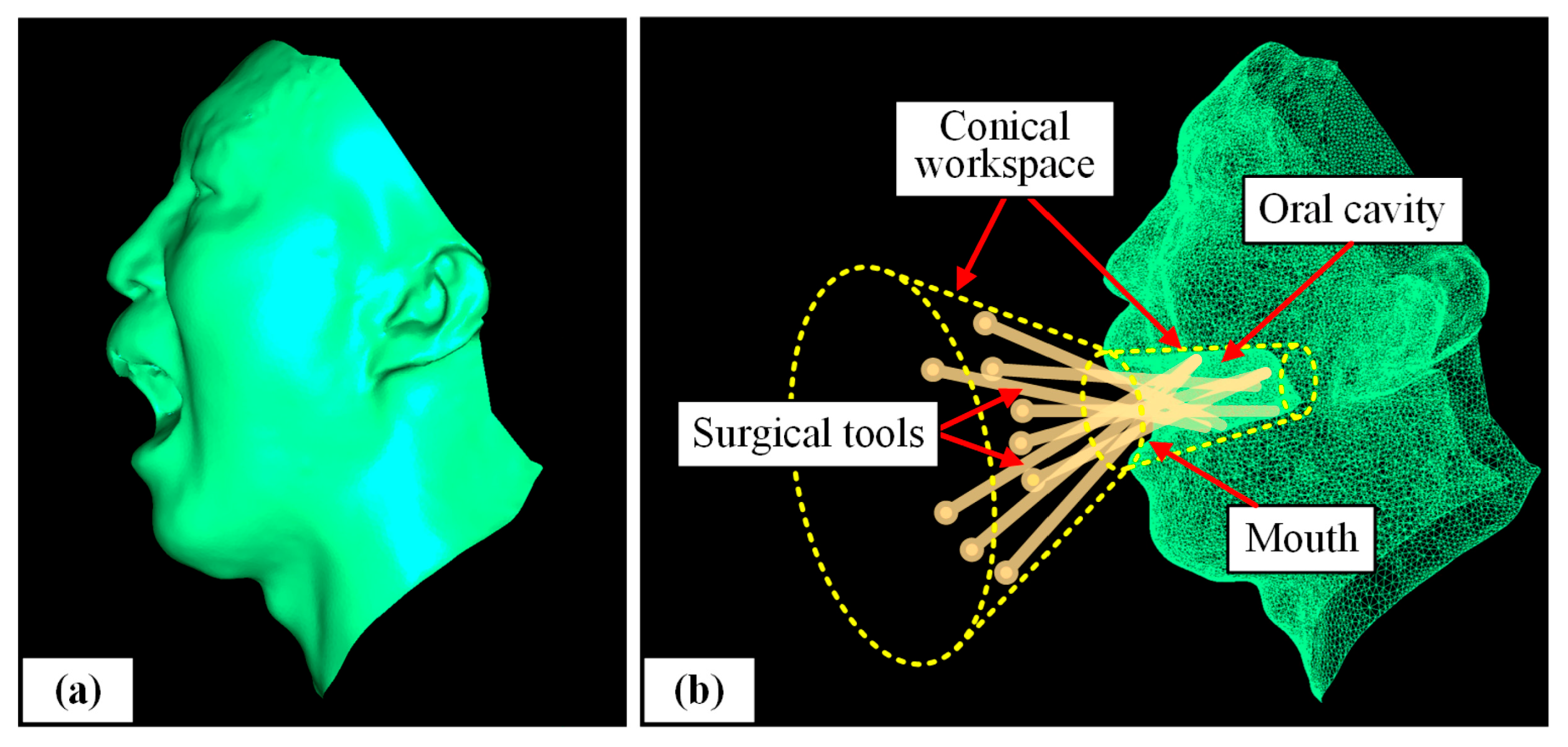
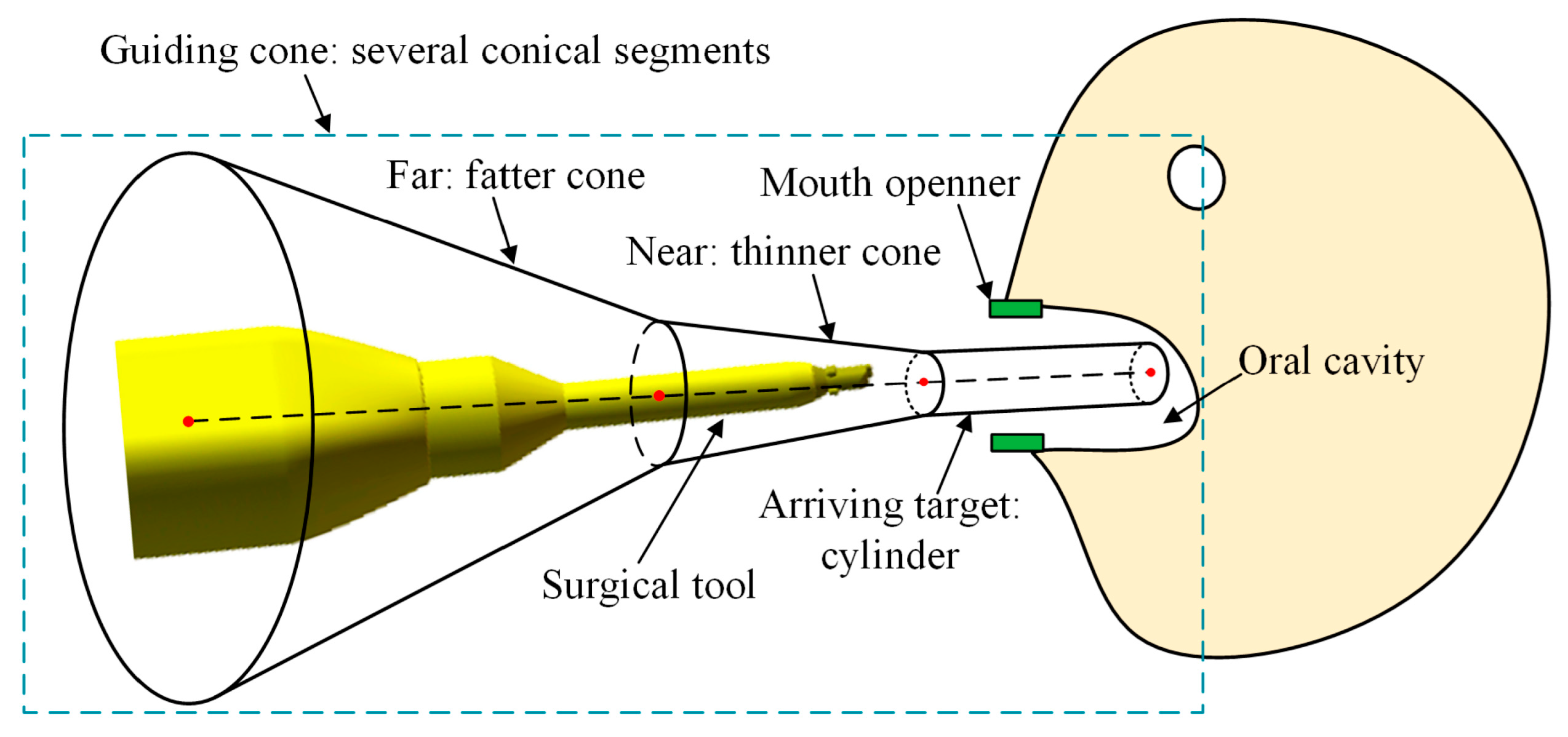
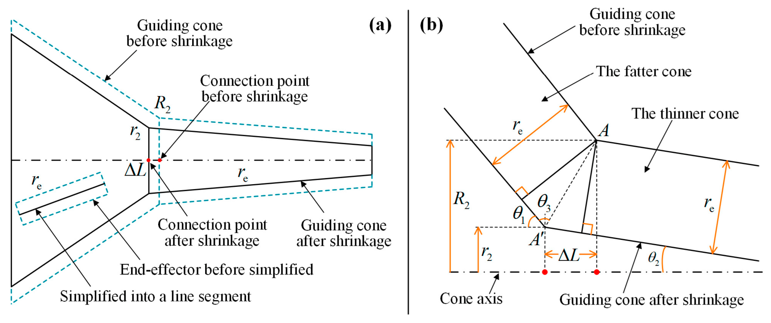
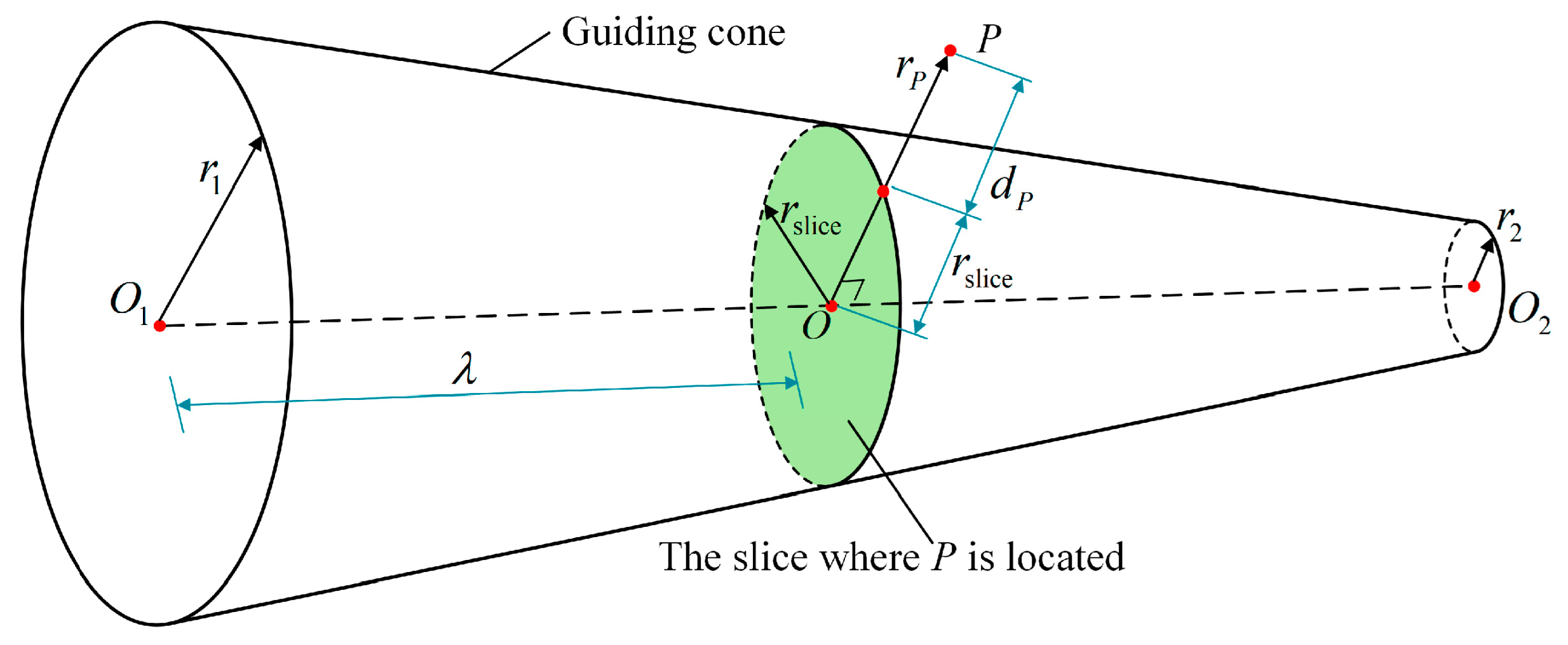
3.1. Geometry of Guiding Cone

A scanned model of a volunteer’s head (including oral cavity) is shown in Figure 3a. In Figure 3b, several surgical tools are simultaneously inserted into the oral cavity. It can be seen that under the geometric configuration of oral surgery, the obstacle avoidance workspace of the surgical tool is similar to two cones, which is the basis to design a VF.

As shown in Figure 4, the guiding cone consists of several conical segments connected together. When the tool is far from the target, the guiding cone is fat and has a larger free space. When the tool is closed to the mouth, the guiding cone becomes thinner, and the motion is gradually constrained. When the tool approaches or reaches the target, the guiding cone shrinks into a cylinder which totally limits the position and orientation of the surgical tool. This design provides a certain free space for manual operation and constrains the undesired motion, which is in accordance with the geometric conditions of oral surgery. Besides, the guiding cone can not only constrain the position of the surgical tool, but also can correct the orientation, which is essential for accurate positioning.

The surgical tool is similar to a cylindrical rod, and different tools have different radii. In order to efficiently calculate the position relationship between the tool and the guiding cone, the tool (cylinder) should be simplified into a line segment. To do this, the guiding cone needs to shrink the radius of the tool inward, as shown in Figure 5a. It can be seen that the connection point of two adjacent cones moves backward by ${\Delta }L$, and the radius of the connection of two adjacent cones shrinks from $R_{2 }$ to $r_2$. The geometric relationship of the shrinkage is shown in Figure 5b by which the parameters ${\Delta }L$ and $r_{2 }$ can be obtained as shown in Equations (5) and (6). After radius compensation (shrinkage), the surgical instrument is simplified as a line segment, which brings convenience to the calculation of the position relationship described later. In the subsequent discussion on the virtual repulsive force and the effect of the guiding cone (Section 3.2 and Section 4), it is assumed that the end effector is simplified into a line segment and the guiding cone is shrunk inward by the radius of the surgical tool.

$$r_2=R_2-r_{\mathrm{e}}\left(\cos {\theta }_1+\tan \left(\frac{{\theta }_1-{\theta }_2}{2}\right)\sin {\theta }_1\right)$$

(5)

$${\Delta }L=r_{\mathrm{e}}\sin \left(\frac{{\theta }_1+{\theta }_2}{2}\right)/\cos \left(\frac{{\theta }_1-{\theta }_2}{2}\right)$$

(6)

where $R_2$ and $r_2$ are the radius of the connection of two adjacent cones, $R_2$ represents the original radius, $r_2$ represents the shrunk radius, $r_{\mathrm{e}}$ is the radius of the surgical tool, ${\Delta }L$ is the movement of the connection point of two adjacent cones, and ${\theta }_1$ and ${\theta }_2$ are the cone angles of two adjacent cones.

3.2. Distance and Repulsive Force

The distance from a point $P$ to the guiding cone is key to generate repulsive force and exert adjustment effect. To simplify the definition, the distance is defined by the direction vertical to the cone axis, not the distance from the point to the surface. In other words, the distance is defined on a slice of the guiding cone. The definition is shown in Figure 6, and distance is given in Equations (7) and (8).

$$\lambda =\overrightarrow{O_1{O}_2}\cdot \overrightarrow{O_{1}P}/{‖\overrightarrow{O_1{O}_2}‖}^2$$

(7)

$$\begin{array}{ll}{d}_P& =r_P-r_{\mathrm{slice}}\\ & =‖\overrightarrow{O_{1}P}-\lambda \overrightarrow{O_1{O}_2}‖-\left(r_1+\lambda \left(r_2-r_1\right)\right)\end{array}$$

(8)

where $\lambda$ is the ratio of the slice where point $P$ is located to the height of the cone, $d_P$ is the distance point $P$ exceeds the guiding cone, $r_P$ represents the length of OP which is the distance from $P$ to the slice center $O$, $r_{\mathrm{silce}}$ is the radius of the slice, and $r_1$ and $r_2$ are the two radii of one segment of the guiding cone.

If the end-effector is beyond the guiding cone, it will be subject to repulsive forces, pushing it back into the guiding cone. The magnitude of the repulsive force is related to the distance (the direction will be discussed in Section 4). The repulsive force can be divided into the free phase, the transition phase, and the maximum repulsive phase according to the distance. For point $P$ in Figure 6, in the free phase, the point is inside the guiding cone, the repulsive force remains 0, and the point $P$ can move freely. In the transition phase, the point starts to exceed the guiding cone, and the repulsive force gradually increases from 0, trying to push the point $P$ back to the guiding cone. In the maximum repulsive phase, the repulsive force reaches the maximum but does not continue to increase to avoid excessive response. The relationship between the magnitude of the repulsive force and the distance is shown in Equation (9).

$$F_{\mathrm{rep}}=\left\{\begin{array}{l}0\hspace{1em}(d_P<0)\\ 1-\cos \left(0.5\pi d_P/d_{\max }\right)\hspace{1em}(0\le d_P\le d_{\max })\\ 1\hspace{1em}(d_P>1)\end{array}\right.$$

(9)

where $F_{\mathrm{rep}}$ is the the magnitude of the repulsive force, $d_{\max }$ is the distance at which the repulsive force will no longer increase. The repulsive force and its relationship with $d_P$ is also shown in Figure 7.

4. Effect of Guiding Cone

4.1. Two-Point Adjustment Model

In the effect of the guiding cone, since the surgical tool is shrunk to a line segment, it can be simplified into two points: a top end $T$ and a far end $F$. Repulsive forces will be inflicted on the two endpoints, and then the repulsive forces will be converted to their respective adjustment velocities ${\mathit{v}}_{\mathrm{far}}^{\left(\mathrm{adj}\right)}$ and ${\mathit{v}}_{\mathrm{far}}^{\left(\mathrm{adj}\right)}$, so as to push the tool back into the guiding cone. The above is the two-point adjustment model, as shown in Figure 8.

For the repulsive force, after the magnitude is discussed in Section 3.2, the direction will be defined here, as shown in Figure 9. For the repulsive force of the top end $T$, in order not to interfere with the motion along the guiding cone axis $\overline{ O_1{O}_2}$, the direction vector ${\mathit{D}}_{top }$ is toward the slice center $O_T$ (along vector $\overrightarrow{T{O}_T}$), and the component along the guiding cone axis $\overline{ O_1{O}_2}$ is 0. For the repulsive force at the far end $F$ of the surgical tool, its direction vector ${\mathit{D}}_{far }$ is defined in plane $\gamma$ that is vertical to the surgical tool (line segment $\overline{FT}$), so that the component along the tool direction $\overrightarrow{FT}$ is 0. Following that, the direction of the repulsive force at the far end $F$ is defined as the projection vector that vector $\overrightarrow{F{O}_F}$ projected on plane $\gamma$, where vector $\overrightarrow{F{O}_F}$ is from the far end $F$ to the corresponding slice center $O_F$.

Based on the vector projection matrix, the direction of the repulsive force on the two endpoints can be obtained as Equations (10) and (11).

$$\begin{array}{ll}{D}_{\mathrm{top}}& =P_{\mathrm{OT}}-P_{\mathrm{T}}\\ & =P_{\mathrm{O}1}+\frac{n\cdot n^{\mathrm{T}}}{n^{\mathrm{T}}\cdot n}\cdot \left(P_{\mathrm{T}}-P_{\mathrm{O}1}\right)-P_{\mathrm{T}}\end{array}$$

(10)

where ${\mathit{D}}_{\mathrm{top}}$ is the 3D direction vector of the repulsive force on the top point, ${\mathit{P}}_{\mathrm{OT}}$, ${\mathit{P}}_{\mathrm{O}1}$, are the coordinate of points $O_{\mathrm{T}}$,$O_1$; $\mathit{n}$ represents the vector $\overrightarrow{O_1{O}_2}$.

$$\begin{array}{ll}{D}_{\mathrm{far}}& =\left(I-\frac{t\cdot t^{\mathrm{T}}}{t^{\mathrm{T}}\cdot t}\right)\cdot \left(P_{\mathrm{OF}}-P_{\mathrm{F}}\right)\\ & =\left(I-\frac{t\cdot t^{\mathrm{T}}}{t^{\mathrm{T}}\cdot t}\right)\cdot \left(P_{\mathrm{O}1}+\frac{n\cdot n^{\mathrm{T}}}{n^{\mathrm{T}}\cdot n}\cdot \left(P_{\mathrm{F}}-P_{\mathrm{O}1}\right)-P_{\mathrm{F}}\right)\end{array}$$

(11)

where ${\mathit{D}}_{\mathrm{far}}$ is the direction vector of the repulsive force on the far point, $\mathit{t}$ represents the tool’s vector $\overrightarrow{FT}$. ${\mathit{P}}_{\mathrm{OF}}$ is the coordinate of point $O_{\mathrm{F}}$. Thus, the repulsive forces ${\mathit{F}}_{\mathrm{top}}$ and ${\mathit{F}}_{\mathrm{far}}$ can be expressed as:

$$\left\{\begin{array}{l}{F}_{\mathrm{top}}=F_{\mathrm{rep}}\cdot D_{\mathrm{top}}/‖D_{\mathrm{top}}‖\\ F_{\mathrm{far}}=F_{\mathrm{rep}}\cdot D_{\mathrm{far}}/‖D_{\mathrm{far}}‖\end{array}\right.$$

(12)

Following that, the adjustment velocities ${\mathit{v}}_{\mathrm{top}}^{\left(\mathrm{adj}\right) }$ and ${\mathit{v}}_{\mathrm{far}}^{\left(\mathrm{adj}\right)}$ can be obtained by a gain $\mathsf{\alpha }$ that converts the repulsive force to the adjustment velocity:

$$\left\{\begin{array}{l}{v}_{\mathrm{top}}^{(\mathrm{adj})}=\alpha \cdot F_{\mathrm{top}}\\ v_{\mathrm{far}}^{(\mathrm{adj})}=\alpha \cdot F_{\mathrm{far}}\end{array}\right.$$

(13)

Furthermore, there is one special situation that needs to be briefly explained. In this situation, the tool crosses two or more guiding cone segments, in other words, the far end $F$ is behind the slice where $O_1$ is located. Under the situation, the point $F$ should be deactivated, and take the intersection point of the $O_1$ slice and the tool to be the new far end $F$, so as to make the two endpoints subjected to one guiding cone segment and avoid the tool crossing the boundary at the connection of two guide cone segments.

The above is the content of the two-point adjustment model which has the following two advantages. First, since the two endpoints of the line are the most likely to go beyond a cone among the line segment, examining the two endpoints is sufficient and the most efficient way. Second, the orientation of the surgical tool can be effectively adjusted through the two endpoints.

4.2. Velocity Conversion

As the second part of the guiding cone’s effect, the velocity conversion is a process that converts the adjustment velocity of the surgical tool obtained in Equation (13) into the joint space of the manipulator which is the plant to directly perform the motion. First, we used the Denavit–Hartenberg method to build the forward kinematics model [42]. The coordinate systems of the joints are shown in Figure 10, where a T-shape connector is used to mount the surgical tool on the mounting flange, and a coordinate system $\left\{End\right\}$ is fixed on the top end of the tool. The forward kinematics is expressed in Equation (14).

$${}_{\mathrm{e}}{}^{\mathrm{b}}T={}_1{}^{\mathrm{b}}T{}_2{}^{1}T\cdots {}_6{}^{5}T{}_{\mathrm{e}}{}^{6}T=\left(\begin{array}{cc}{}_{\mathrm{e}}{}^{\mathrm{b}}R& P_{\mathrm{end}}\\ O& 1\end{array}\right)$$

(14)

where ${}_{\mathrm{e}}{}^{ \mathrm{b}}\mathit{T}$ is the transformation matrix from the base coordinate system $\left\{Base\right\}$ to the end coordinate system $\left\{End\right\}$, ${}_{\mathrm{e}}{}^{ \mathrm{b}}\mathit{R}$ and ${\mathit{P}}_{\mathrm{end}}$ are the corresponding rotation matrix and position vector of top point of the tool, and ${}_{\mathrm{e}}{}^{ 6}\mathit{T}$ is the transformation matrix from the the mounting flange to the end point of the tool.

The adjustment velocities ${\mathit{v}}_{\mathrm{top}}^{\left(\mathrm{adj}\right) }$ and ${\mathit{v}}_{\mathrm{far}}^{\left(\mathrm{adj}\right)}$ of the surgical tool are described in the base coordinate system $\left\{Base\right\}$. In order to describe the rigid body motion of the tool, transfer ${\mathit{v}}_{\mathrm{top}}^{\left(\mathrm{adj}\right) }$ and ${\mathit{v}}_{\mathrm{far}}^{\left(\mathrm{adj}\right)}$ to the end coordinate system $\left\{End\right\}$ to get the adjustment velocities ${}_{}{}^{\mathrm{e}}\mathit{v}{}_{\mathrm{top}}^{\left(\mathrm{adj}\right) }$ and ${}_{}{}^{\mathrm{e}}\mathit{v}{}_{\mathrm{far}}^{\left(\mathrm{adj}\right) }$ that was described in $\left\{End\right\}$.

$$\left\{\begin{array}{l}{}_{}{}^{\mathrm{e}}v{}_{\mathrm{far}}^{\left(\mathrm{adj}\right)}={}_{\mathrm{b}}{}^{\mathrm{e}}R\cdot v_{\mathrm{far}}^{\left(\mathrm{adj}\right)}={\left({}_{\mathrm{e}}{}^{\mathrm{b}}R\right)}^{\mathrm{T}}\cdot v_{\mathrm{far}}^{\left(\mathrm{adj}\right)}\\ {}_{}{}^{\mathrm{e}}v{}_{\mathrm{top}}^{\left(\mathrm{adj}\right)}={}_{\mathrm{b}}{}^{\mathrm{e}}R\cdot v_{\mathrm{far}}^{\left(\mathrm{adj}\right)}={\left({}_{\mathrm{e}}{}^{\mathrm{b}}R\right)}^{\mathrm{T}}\cdot v_{\mathrm{top}}^{\left(\mathrm{adj}\right)}\end{array}\right.$$

(15)

Next, the adjustment angular velocity of the rigid body motion can be expressed as:

$$\left\{\begin{array}{l}{}_{}{}^{\mathrm{e}}\omega {}_{\mathrm{x}}^{(\mathrm{adj})}=0\\ {}_{}{}^{\mathrm{e}}\omega {}_{\mathrm{y}}^{(\mathrm{adj})}=\left({}_{}{}^{\mathrm{e}}\mathit{v}{}_{\mathrm{far},\mathrm{z}}^{(\mathrm{adj})}-{}_{}{}^{\mathrm{e}}\mathit{v}{}_{\mathrm{top},\mathrm{z}}^{(\mathrm{adj})}\right)/d\\ {}_{}{}^{\mathrm{e}}\omega {}_{\mathrm{z}}^{(\mathrm{adj})}=-\left({}_{}{}^{\mathrm{e}}\mathit{v}{}_{\mathrm{far},\mathrm{y}}^{(\mathrm{adj})}-{}_{}{}^{\mathrm{e}}\mathit{v}{}_{\mathrm{top},\mathrm{y}}^{(\mathrm{adj})}\right)/d\end{array}\right.$$

(16)

where ${}_{}{}^{\mathrm{e}}\omega {}_{\mathrm{x}}^{\left(\mathrm{adj}\right) }$,${}_{}{}^{\mathrm{e}}\omega {}_{\mathrm{y}}^{\left(\mathrm{adj}\right) }$,${}_{}{}^{\mathrm{e}}\omega {}_{\mathrm{z}}^{\left(\mathrm{adj}\right) }$ are the x, y, and z components, respectively, of adjustment angular velocity described in $\left\{End\right\}$, and $d$ is the tool length shown in Figure 10. Then, the 6-dimension velocity vector ${}_{}{}^{\mathrm{e}}\mathit{V}{}_{\mathrm{adj}}$ of the tool described in $\left\{End\right\}$ can be written as:

$$\begin{array}{ll}{}_{}{}^{\mathrm{e}}V{}_{\mathrm{adj}}& ={\left({}_{}{}^{\mathrm{e}}v{}_{\mathrm{top}}^{(\mathrm{adj})},{}_{}{}^{\mathrm{e}}\omega {}_{\mathrm{x}}^{(\mathrm{adj})},{}_{}{}^{\mathrm{e}}\omega {}_{\mathrm{y}}^{(\mathrm{adj})},{}_{}{}^{\mathrm{e}}\omega {}_{\mathrm{z}}^{(\mathrm{adj})}\right)}^{\mathrm{T}}\\ & ={\left({}_{}{}^{\mathrm{e}}\mathit{v}{}_{\mathrm{x}}^{(\mathrm{adj})},{}_{}{}^{\mathrm{e}}\mathit{v}{}_{\mathrm{y}}^{(\mathrm{adj})},{}_{}{}^{\mathrm{e}}\mathit{v}{}_{\mathrm{z}}^{(\mathrm{adj})},{}_{}{}^{\mathrm{e}}\omega {}_{\mathrm{x}}^{(\mathrm{adj})},{}_{}{}^{\mathrm{e}}\omega {}_{\mathrm{y}}^{(\mathrm{adj})},{}_{}{}^{\mathrm{e}}\omega {}_{\mathrm{z}}^{(\mathrm{adj})}\right)}^{\mathrm{T}}\end{array}$$

(17)

where ${}_{}{}^{\mathrm{e}}\mathit{v}{}_{\mathrm{x}}^{\left(\mathrm{adj}\right) }$,${}_{}{}^{\mathrm{e}}\mathit{v}{}_{\mathrm{y}}^{\left(\mathrm{adj}\right) }$,${}_{}{}^{\mathrm{e}}\mathit{v}{}_{\mathrm{z}}^{\left(\mathrm{adj}\right) }$ are the x, y, and z components, respectively, of the adjustment velocity ${}_{}{}^{\mathrm{e}}\mathit{v}{}_{\mathrm{top}}^{\left(\mathrm{adj}\right) }$ of the top end on the tool described in $\left\{End\right\}$.

In order to convert the 6-dimension velocity vector ${}_{}{}^{\mathrm{e}}\mathit{V}{}_{\mathrm{adj}}$ of the tool into the joint space of the manipulator, the Jacobian matrix of the manipulator should be involved, which can be obtained from the forward kinematics result in Equation (14):

$${}_{}{}^{\mathrm{b}}J=\left(\begin{array}{cccc}\frac{\partial p_{\mathrm{end}}}{\partial {\theta }_1}& \frac{\partial p_{\mathrm{end}}}{\partial {\theta }_2}& \cdots & \frac{\partial p_{\mathrm{end}}}{\partial {\theta }_6}\\ \frac{\partial r_3}{\partial {\theta }_1}{r}_2^{\mathrm{T}}& \frac{\partial r_3}{\partial {\theta }_2}{r}_2^{\mathrm{T}}& \cdots & \frac{\partial r_3}{\partial {\theta }_6}{r}_2^{\mathrm{T}}\\ \frac{\partial r_1}{\partial {\theta }_1}{r}_3^{\mathrm{T}}& \frac{\partial r_1}{\partial {\theta }_2}{r}_3^{\mathrm{T}}& \cdots & \frac{\partial r_1}{\partial {\theta }_6}{r}_3^{\mathrm{T}}\\ \frac{\partial r_2}{\partial {\theta }_1}{r}_1^{\mathrm{T}}& \frac{\partial r_2}{\partial {\theta }_2}{r}_1^{\mathrm{T}}& \cdots & \frac{\partial r_2}{\partial {\theta }_6}{r}_1^{\mathrm{T}}\end{array}\right)$$

(18)

where ${}_{}{}^{\mathrm{b}}\mathit{J}$ represents the $6\times 6$ Jacobian matrix of the manipulator described in $\left\{Base\right\}$; ${\theta }_1$, ${\theta }_2$, …,${\theta }_6$ are the six joint angles of the manipulator; ${\mathit{r}}_1$, ${\mathit{r}}_2$, ${\mathit{r}}_3$ are the $1\times 3$ row vectors that respectively represents the line 1, 2, 3 of the rotation matrix ${}_{\mathrm{e}}{}^{ \mathrm{b}}\mathit{R}$. Then, transfer the ${}_{}{}^{\mathrm{b}}\mathit{J}$ into the end coordinate system $\left\{End\right\}$ as shown in Equation (19):

$${}_{}{}^{\mathrm{e}}J=\left(\begin{array}{cc}{}_{\mathrm{e}}{}^{\mathrm{b}}R& O\\ O& {}_{\mathrm{e}}{}^{\mathrm{b}}R\end{array}\right)\cdot {}_{}{}^{\mathrm{b}}J$$

(19)

where ${}_{}{}^{\mathrm{e}}\mathit{J}$ represents the $6\times 6$ Jacobian matrix described in $\left\{End\right\}$. After that, the $6\times 1$ adjustment velocity vector ${}_{}{}^{\mathrm{e}}\mathit{V}{}_{\mathrm{adj}}$ can be converted to the joint adjustment velocity vector ${\dot{\mathit{\theta }}}_{\mathrm{adj}}$ as shown in Equation (20).

$${\dot{\theta }}_{\mathrm{adj}}={}_{}{}^{\mathrm{e}}J{}^{+}\cdot {}_{}{}^{\mathrm{e}}V{}_{\mathrm{adj}}$$

(20)

where ${}_{}{}^{\mathrm{e}}\mathit{J}{}^{+}$ is the pseudo inverse matrix of ${}_{}{}^{\mathrm{e}}\mathit{J}$. Finally, the joint angles ${\mathit{\theta }}_{\mathrm{exe}}$, which should be executed by the manipulator, can be derived as follows:

$${\theta }_{\mathrm{exe}}={\theta }_{\mathrm{cmd}}+{\displaystyle {\int }_0^t{\dot{\theta }}_{\mathrm{adj}}}dt$$

(21)

where ${\mathit{\theta }}_{\mathrm{cmd}}$ represents the joint angle command from the master–slave operation. Thus, the effect of the guiding cone is established, and the diagram of the adjustment effect is shown in Figure 11. From Figure 11, it can be seen that design of the guiding cone and the adjustment effect form the complete proposed virtual fixture framework.

5. System Integration of Guiding Cone

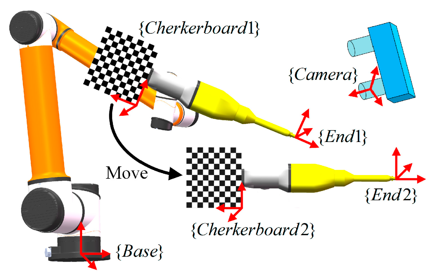
5.1. Calibration and Correction

In OSRS, a binocular vision system and a mouth opener are involved to locate the oral cavity in real time, thereby the guiding cone can be corrected to suit a dynamic target. Since the position and orientation of the detected mouth opener are described in the camera’s coordinate system, hand–eye calibration, as the approach for obtaining the transformation between the manipulator and camera is responsible for obtaining the target’s description in the manipulator’s coordinate system.

In hand–eye calibration, a checkerboard is fixed on the end-effector, shown in Figure 12. To calculate the transformation from $\left\{Base\right\}$ to $\left\{Camera\right\}$, the manipulator should be driven to at least two different positions. Given that the transformation from end-effector to checkerboard remains unchanged regardless of how the manipulator moves, the relation between transformation matrices can be expressed as Equation (22).

$$\left({}_{\mathrm{e}}{}^{\mathrm{b}}T{}^{(2)}{}_{\mathrm{b}}{}^{\mathrm{e}}T{}^{(1)}\right)\cdot {}_{\mathrm{c}}{}^{\mathrm{b}}T={}_{\mathrm{c}}{}^{\mathrm{b}}T\cdot \left({}_{\mathrm{ch}}{}^{\mathrm{c}}T{}^{(2)}{}_{\mathrm{c}}{}^{\mathrm{ch}}T{}^{(1)}\right)$$

(22)

where ${}_{\mathrm{e}}{}^{\mathrm{b}}\mathit{T}{}_{}^{\left(1\right)}$ is the transformation from $\left\{Base\right\}$ to $\left\{End1\right\}$. ${}_{\mathrm{c}}{}^{\mathrm{b}}\mathit{T}$ is the transformation from $\left\{Base\right\}$ to $\left\{Camera\right\}$ to be solved in hand–eye calibration. ${}_{\mathrm{c}}{}^{\mathrm{ch}}\mathit{T}{}_{}^{\left(1\right)}$ is the transformation from $\left\{Checkerboard1\right\}$ to $\left\{Camera\right\}$. Then, ${}_{\mathrm{e}}{}^{\mathrm{b}}\mathit{T}{}_{}^{\left(2\right)}{}_{\mathrm{b}}{}^{\mathrm{e}}\mathit{T}{}_{}^{\left(1\right)}$ and ${}_{\mathrm{ch}}{}^{\mathrm{c}}\mathit{T}{}_{}^{\left(2\right)}{}_{\mathrm{c}}{}^{\mathrm{ch}}\mathit{T}{}_{}^{\left(1\right)}$ can be written as ${\mathit{T}}_{\mathrm{A}}$ and ${\mathit{T}}_{\mathrm{B}}$, respectively, with rotational partitions ${\mathit{R}}_{\mathrm{A}}$, ${\mathit{R}}_{\mathrm{B}}$ and translational partitions ${\mathit{t}}_{\mathrm{A}}$, ${\mathit{t}}_{\mathrm{B}}$ assembled in them. Thereby, the calibration result can be obtained as follows.

$$\begin{array}{l}\left(\left(\begin{array}{ccc}{R}_{\mathrm{A}}& & O\\ & R_{\mathrm{A}}& \\ O& & R_{\mathrm{A}}\end{array}\right)-K\left(\begin{array}{ccc}{R}_{\mathrm{B}}^{\mathrm{T}}& & O\\ & R_{\mathrm{B}}^{\mathrm{T}}& \\ O& & R_{\mathrm{B}}^{\mathrm{T}}\end{array}\right)K\right)r_{\mathrm{X}}=0\\ t_{\mathrm{X}}={\left(R_{\mathrm{A}}-I\right)}^{-1}\left(R_{\mathrm{X}}{t}_{\mathrm{B}}-t_{\mathrm{A}}\right)\end{array}$$

(23)

where ${\mathit{R}}_{\mathrm{X}}$ and ${\mathit{t}}_{\mathrm{X}}$ are, respectively, rotational and translational partitions of ${}_{\mathrm{c}}{}^{\mathrm{b}}\mathit{T}$, and ${\mathit{r}}_{\mathrm{X}}={\left(r_{11},r_{21},r_{31},\cdots ,r_{23},r_{33}\right)}^{\mathrm{T}}$ is the vectorized expression of ${\mathit{R}}_{\mathrm{X}}$ and can be calculated by using SVD decomposition. $\mathit{K}$ is a $9\times 9$ constant matrix with elements in column 1, 4, 7, 2, 5, 8, 3, 6, 9 of line 1 to 9, respectively, are one, and all other elements are zero.

The guiding cone can be determined by “anchor-arrow” description: an anchor point and an arrow (3D vector) represent the position and orientation, respectively. The “anchor-arrow” description is preoperatively defined under the mouth opener’s local coordinate system whose transformation to the camera’s coordinate system can be obtained from the vision system. To convert the “anchor-arrow” description from the mouth opener to the manipulator, the hand–eye calibration result is necessary. The correction of the guiding cone is shown in Figure 13, Equations (24) and (25).

$$\left\{\begin{array}{l}{}_{}{}^{\mathrm{b}}P{}_{\mathrm{an}}={}_{\mathrm{c}}{}^{\mathrm{b}}T\cdot {}_{\mathrm{op}}{}^{\mathrm{c}}T\cdot {}_{}{}^{\mathrm{op}}P{}_{\mathrm{an}}\\ {}_{}{}^{\mathrm{b}}D{}_{\mathrm{ar}}={}_{\mathrm{c}}{}^{\mathrm{b}}T\cdot {}_{\mathrm{op}}{}^{\mathrm{c}}T\cdot {}_{}{}^{\mathrm{op}}D{}_{\mathrm{ar}}\end{array}\right.$$

(24)

$${}_{}{}^{\mathrm{b}}P{}_{\mathrm{o}}={}_{}{}^{\mathrm{b}}P{}_{\mathrm{an}}+{}_{}{}^{\mathrm{b}}D{}_{\mathrm{ar}}\cdot l_{\mathrm{an}}/‖{}_{}{}^{\mathrm{b}}D{}_{\mathrm{ar}}‖$$

(25)

where ${}_{}{}^{\mathrm{b}}\mathit{P}{}_{\mathrm{an}}$ and ${}_{}{}^{\mathrm{op}}\mathit{P}{}_{\mathrm{an}}$ are the positions of the anchor point described in $\left\{Base\right\}$ and $\left\{Opener\right\}$, respectively, and ${}_{}{}^{\mathrm{b}}\mathit{D}{}_{\mathrm{an}}$ and ${}_{}{}^{\mathrm{op}}\mathit{D}{}_{\mathrm{an}}$ are the direction vectors of the arrow under $\left\{Base\right\}$ and $\left\{Opener\right\},$ respectively. ${}_{\mathrm{c}}{}^{\mathrm{b}}\mathit{T}$ is the hand–eye calibration result. ${}_{\mathrm{op}}{}^{\mathrm{c}}\mathit{T}$ is the transformation from $\left\{Camera\right\}$ to $\left\{Opener\right\}$ obtained from the vision system. ${}_{}{}^{\mathrm{b}}\mathit{P}{}_{\mathrm{o}}$ is an arbitrary slice’s center in Figure 6 under $\left\{Base\right\}$, and $l_{\mathrm{an}}$ is the distance between a slice’s center and the anchor point. With the “anchor-arrow” description, a guiding cone can be fully defined when the radii and distances of all the slices are given.

5.2. Automatic Feeding Mode

If no obstacles are inside the guiding cone, an optional automatic mode may be preferable. In the automatic mode, the master–slave motion command is replaced by position and orientation interpolation, and then the guiding cone can adjust the interpolated motion command to ensure safety. The intermediate points can be expressed as follows, in which the position is directly interpolated, and the orientation is smoothly interpolated by using the rotation vector method:

$$\left\{\begin{array}{l}{}_{}{}^{\mathrm{b}}P{}_t={}_{}{}^{\mathrm{b}}P{}_{\mathrm{init}}+u(t)\left({}_{}{}^{\mathrm{b}}P{}_{\mathrm{aim}}-{}_{}{}^{\mathrm{b}}P{}_{\mathrm{init}}\right)\\ {}_{}{}^{\mathrm{b}}R{}_t={}_{}{}^{\mathrm{b}}R{}_{\mathrm{init}}\cdot mat\left(u(t)\cdot vec\left({}_{}{}^{\mathrm{b}}R{}_{\mathrm{init}}^{-1}\cdot {}_{}{}^{\mathrm{b}}R{}_{\mathrm{aim}}\right)\right)\end{array}\right.$$

(26)

where ${}_{}{}^{\mathrm{b}}\mathit{P}{}_t$, ${}_{}{}^{\mathrm{b}}\mathit{P}{}_{\mathrm{init}}$, and ${}_{}{}^{\mathrm{b}}\mathit{P}{}_{\mathrm{aim}}$ are the end-effector’s positions of time $t$, time 0, and the destination, respectively, under $\left\{Base\right\}$. ${}_{}{}^{\mathrm{b}}\mathit{R}{}_t$, ${}_{}{}^{\mathrm{b}}\mathit{R}{}_{\mathrm{init}}$, and ${}_{}{}^{\mathrm{b}}\mathit{R}{}_{\mathrm{aim}}$ are corresponding destination’s orientations. $mat$ and $vec$ are conversion functions between rotation matrix and rotation vector. $u\left(t\right)$ is a normalized time factor as well as a monotonic function whose variable is time $t$, when $t=0$, $u\left(t\right)=0$, and when $t\ge end$, $u\left(t\right)=1$.

Meanwhile, with the mouth opener, ${}_{}{}^{\mathrm{b}}\mathit{P}{}_{\mathrm{aim}}$ and ${}_{}{}^{\mathrm{b}}\mathit{R}{}_{\mathrm{aim}}$ are refreshed in real time through ${}_{\mathrm{c}}{}^{\mathrm{b}}\mathit{T}$ and ${}_{\mathrm{op}}{}^{\mathrm{c}}\mathit{T}$ obtained from the vision system, as shown in Equation (27).

$${}_{}{}^{\mathrm{b}}T{}_{\mathrm{aim}}={}_{\mathrm{c}}{}^{\mathrm{b}}T\cdot {}_{\mathrm{op}}{}^{\mathrm{c}}T\cdot {}_{}{}^{\mathrm{op}}T{}_{\mathrm{aim}}$$

(27)

where ${}_{}{}^{\mathrm{b}}\mathit{T}{}_{\mathrm{aim}}$ is assembled by ${}_{}{}^{\mathrm{b}}\mathit{P}{}_{\mathrm{aim}}$ and ${}_{}{}^{\mathrm{b}}\mathit{R}{}_{\mathrm{aim}}$, and ${}_{}{}^{\mathrm{op}}\mathit{T}{}_{\mathrm{aim}}$ is the end-effector’s destination under $\left\{Opener\right\}$. In fact, ${}_{}{}^{\mathrm{op}}\mathit{T}{}_{\mathrm{aim}}$ is similar to ${}_{}{}^{\mathrm{op}}\mathit{P}{}_{\mathrm{an}}$ and ${}_{}{}^{\mathrm{op}}\mathit{D}{}_{\mathrm{an}}$, and all of them coincide with each other. The difference is that ${}_{}{}^{\mathrm{op}}\mathit{T}{}_{\mathrm{aim}}$ describes the end-effector, while ${}_{}{}^{\mathrm{op}}\mathit{P}{}_{\mathrm{an}}$ and ${}_{}{}^{\mathrm{op}}\mathit{D}{}_{\mathrm{an}}$ form the “anchor-arrow” to describe the guiding cone.

By now, the system is integrated, forming a complete motion strategy. To sum up, the new conical virtual fixture is established with geometry design and effect mode, and then combined with the vision system to build the overall strategy. Moreover, an optional automatic mode was provided for users. The full strategy is shown in Figure 14.

6. Simulations, Experiments, and Discussion

6.1. Simulations

To verify the feasibility of the proposed virtual fixture, simulations are carried out. To begin with, the virtual fixture consists of four cone segments, whose parameter setups are listed in

Table 1. Parameter setups of the virtual fixture.

Cone	${\mathit{O}}_1$	${\mathit{O}}_2$	${\mathit{r}}_1$	${\mathit{r}}_2$	$\mathsf{\alpha }$	${\mathit{d}}_{\mathbf{m}\mathbf{a}\mathbf{x}}$
1	(900, −550, 620)	(1100, −520, 570)	250 mm	50 mm	150	5 mm
2	(1100, −520, 570)	(1200, −505, 545)	50 mm	10 mm	150	5 mm
3	(1200, −505, 545)	(1300, −490, 520)	10 mm	1 mm	150	5 mm
4	(1300, −490, 520)	(1400, −475, 495)	1 mm	1 mm	150	5 mm

, where $\mathsf{\alpha }$ is the gain in Equation (13) and $d_{\max }$ is the maximum repulsive force layer in Equation (9).

The first simulation group is “static and manual” feeding, that is, the guiding cone is fixed, and the motion is generated by master–slave motion. This group is to verify the adjustment effect, in other words, to check whether the guiding cone can play its role. The results are shown in Figure 15, including the motion process (see Figure 15a,b) and the joint space’s angle (see Figure 15c). The results of the virtual fixture are activated and deactivated (only master–slave command is allowed) are displayed, forming a comparison.

The second simulation group is “dynamic and manual” feeding. In this group, position and orientation of the guiding cone are changing gradually, representing the disturbance of the oral cavity. The original motion command is generated by master–slave operation. When time is 0 s, under the “anchor-arrow” description, the guiding cone’s anchor point is ${\left(1400,-550,620\right)}^{\mathrm{T}}$ and the arrow vector is ${\left(-1,0,0\right)}^{\mathrm{T}}$. When time is 7.5 s, the anchor point is ${\left(1400,-475, 495\right)}^{\mathrm{T}}$ and the arrow vector is ${\left(-0.96,-0.144, 0.24\right)}^{\mathrm{T}}$. The motion process of the tool subjected to a dynamic guiding cone is displayed in Figure 16, from which it can be seen that the surgical tool can still track the guiding cone well and hit the target, although the guiding cone is ever-moving.

In Figure 16, it takes approximately 18 s for the surgical tool to reach the target, and then keeps following the target in the remaining time. Next, the third simulation group is the “static and automatic“ feeding, in which the path is automatically interpolated instead of the master–slave operation, and the guiding cone is fixed. The simulation result is shown in Figure 17. Because direct path interpolation (see Figure 17b) cannot ensure safety, the guiding cone was adopted, as shown in Figure 17a, and the path can be limited inside the guiding cone, eliminating almost all the out-of-range motion that may collide with obstacles. Moreover, from Figure 17c, it can be seen that the trajectory of automatic mode is more smooth than manual operation, making this mode more preferable to some extent.

In addition, the fourth simulation group is the “dynamic and automatic“ feeding. However, all else being equal, the simulated process is just the same as Figure 16 that can sufficiently represent the “dynamic and automatic” feeding process. Therefore, the figure to show this group can be omitted.

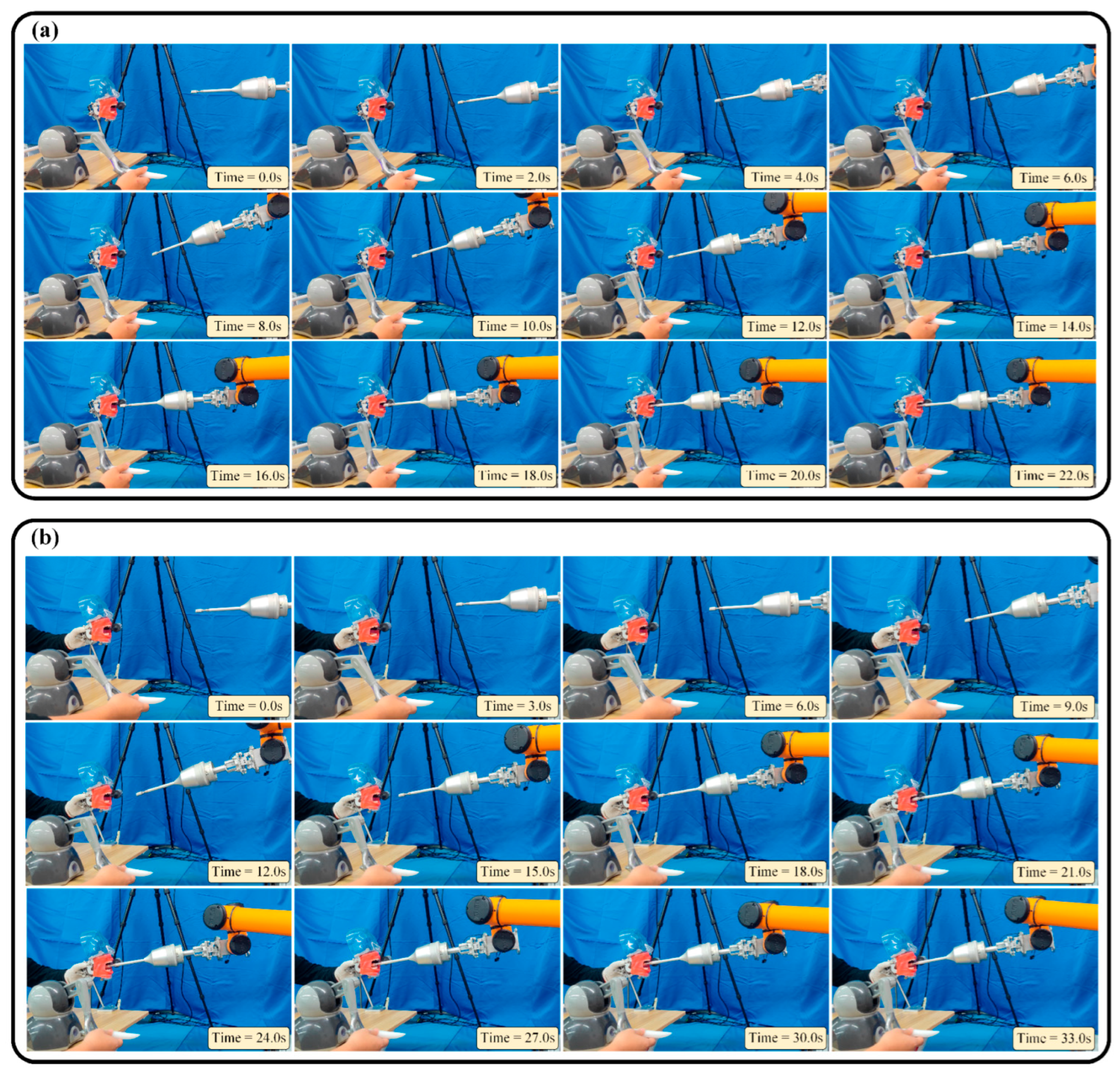
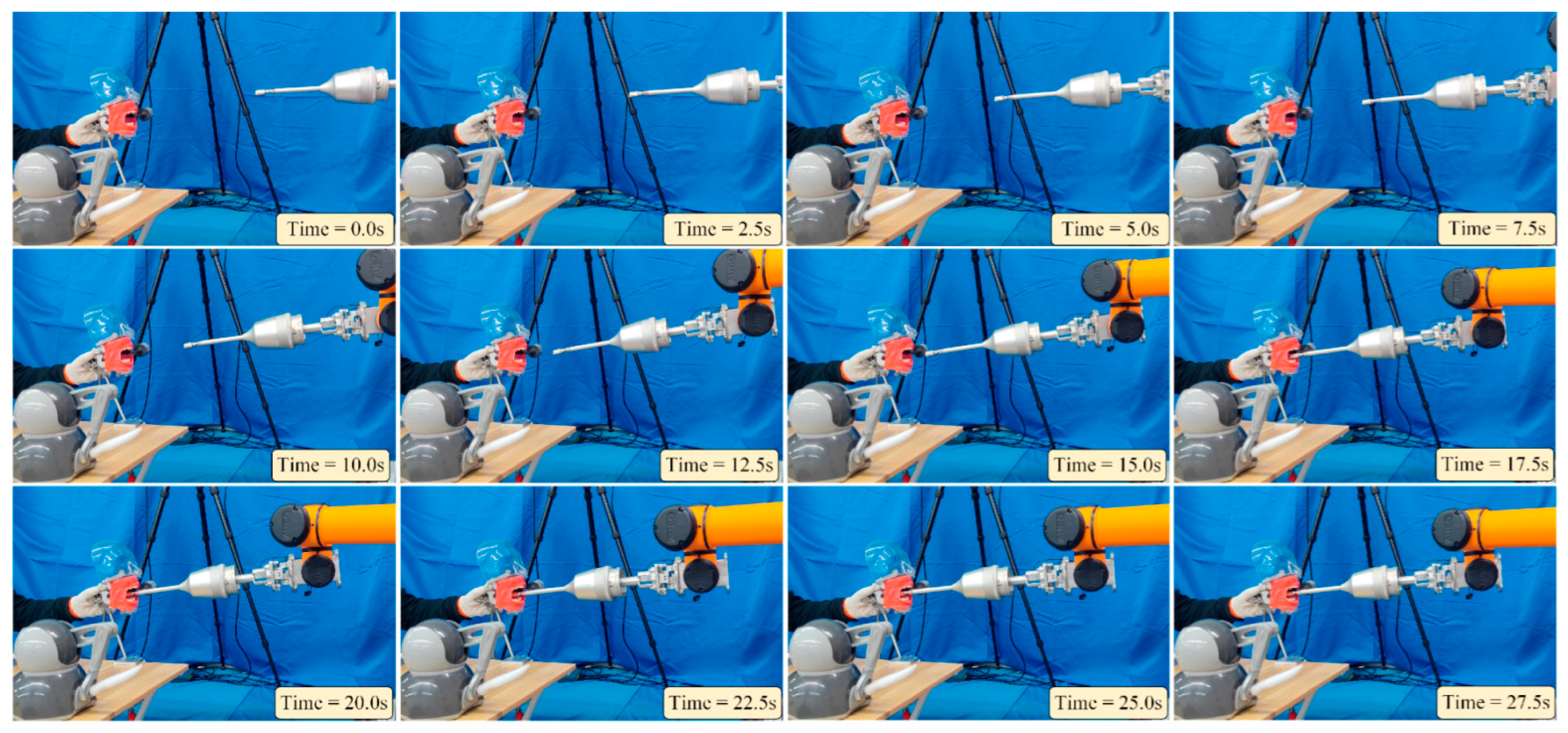
6.2. Experiments

Following the simulations, experiments on an oral model were conducted. Different from the simulations in which only the virtual fixture is concerned, the experiments involve the full strategy where the virtual fixture and vision system are combined. The setup of the experiments is shown in Figure 18. The user grasps the master controller, while another hand shakes the oral model to generate the disturbance motion, with a mouth opener worn on the oral model. The anchor-arrow description of the target is preoperatively defined. The camera calibration and hand–eye calibration is all done. The virtual fixture, as well as the full strategy, is programmed with C++ and runs on an industrial computer with Intel(R) Core(TM) i9-12900H at 2.5 GHz and 32 GB RAM in a 64bit win10 system. The parameters of the virtual fixture are the same as Table 1.

Experiments are conducted with the following three groups: static and manual feeding, dynamic and manual feeding, and dynamic and automatic feeding. The motion process of the three groups is shown in Figure 19a,b and Figure 20, respectively.

In Figure 19a, it takes about 22 s for the surgical tool to reach the target. In Figure 19b, it takes about 24 s to reach the target, and then follows the target in the remaining time. In Figure 20, it takes approximately 20 s to reach the target and then follow it. From the motion processes of the three groups, it can be seen that the motion strategy can successfully guide the surgical tool into the target position inside the oral cavity. Even if the oral cavity is ever-moving, the surgical tool can still hit the target and actively follow the disturbance motion of the oral model, illustrating the effectiveness of the virtual fixture and the motion strategy that is combined with the vision system.

6.3. Discussion

To further discuss the results, the detailed data of the experiments and simulations were extracted and visualized. The motion errors of some groups, which are the distance between the target under anchor-arrow description (also the anchor-arrow description of the guiding cone) and the end-effector, are shown in Figure 21. The disturbances of the target during dynamics groups (shaken by hand) are shown in Figure 22.

From Figure 21a,c, it can be seen that the motion process can be divided into two stages: the feeding stage and the following stage. During the feeding stage, the surgical tool continuously moves forward, and the error declines gradually. During the following stage, the surgical tool reaches the target and remains to keep up with it, making the error close to zero as shown in Figure 21b,d, which are the local magnified figure of the following stage. Then, the average positioning errors in the following stage, including position and orientation, can be obtained as shown in

Table 2. Average positioning error of different groups.

Type	Operation	Target	Average Positioning Error
Experiment	Manual	Static	0.366 mm and 0.227 deg
Experiment	Manual	Dynamic	0.977 mm and 1.017 deg
Experiment	Automatic	Dynamic	0.912 mm and 0.677 deg
Simulation	Manual	Static	0.202 mm and 0.082 deg
Simulation	Manual	Dynamic	0.439 mm and 0.289 deg

, reflecting the extent of accuracy of the motion strategy.

From Table 2, it can be seen that the errors of experiments are obviously larger than that of simulations where the virtual fixture is stand-alone without connecting to the vision system. The extra error between simulations and experiments is induced by the measurement noise from the vision system, which is generally larger when the oral model is dynamic and smaller when the oral model is static. In other words, the guiding cone (or the target) is ever-swinging by the measurement noise during the task, making errors all the time, despite a filter being applied to alleviate the noise.

Besides, there are additional errors between static feeding and dynamic feeding, which are caused by the random disturbances of the oral model. The disturbances are displayed in Figure 22. To follow disturbance motion, a lag is inevitable since it must take a small time interval for the guiding cone to exert its adjusting effect. Therefore, the error is triggered. Relatively more noise of vision measure also contributes to the additional errors between static feeding and dynamic feeding. Moreover, compared with manual operation, automatic mode will make relatively fewer orientation errors (angle error), in that automatic trajectory generation will bring more targeted origin commands than that of manual operation.

In addition, what must be declared here is that error is only defined by the distance between the target read from the vision measurement and the surgical tool. The error is just on behalf of the guiding cone, not the absolute error, which is influenced by hand–eye calibration and accuracy of the vision system. Therefore, the above accuracy data are only to evaluate the virtual fixture itself. If the absolute error is to be obtained, a third-party measurement equipment might be required.

Despite a few errors that still exist, the accuracy of the proposed virtual fixture is sufficient anyway, given that the average following error is less than 1.0 mm and 1.05 deg during a dynamic process in which the oral model is intentionally shaken, as shown in Figure 22a,b. Because the oral disturbance is usually less than the intentional shaking, the error will be less in a real task. The results show that the proposed virtual fixture, as well as the motion strategy, is an effective way to execute the feeding task and fulfill the requirement of oral surgery. To sum up, the position and orientation accuracy can be well guaranteed with the help of the proposed strategy, no matter whether the oral cavity is static or moving. Therefore, the method can simplify a skill-demanding task into an easy task, eliminating the concern of feeding to a wrong position or misoperation. Moreover, the trait of dynamic compensation has the potential to reduce the extra damage to the oral tissue during the surgery.

7. Conclusions and Future Work

This paper introduces a guiding and positioning strategy for robot-assisted oral surgery. The work is conducted during geometry design, effect design, system integration, simulations, and experiments. Conclusions can be listed as follows:

• A new conical virtual fixture, also called the guiding cone, is designed according to the structure of the oral cavity, making it suitable for robot-assisted oral surgery.
• The effect mode of the virtual fixture is established through two-point adjustment and velocity conversion, which can actively adjust the position and orientation of the surgical tool simultaneously.
• The virtual fixture is integrated with a vision system to compensate for the disturbance of the oral cavity. The system calibration is done, the master–slave mapping is combined, and an automatic mode is adopted, forming a complete motion strategy.
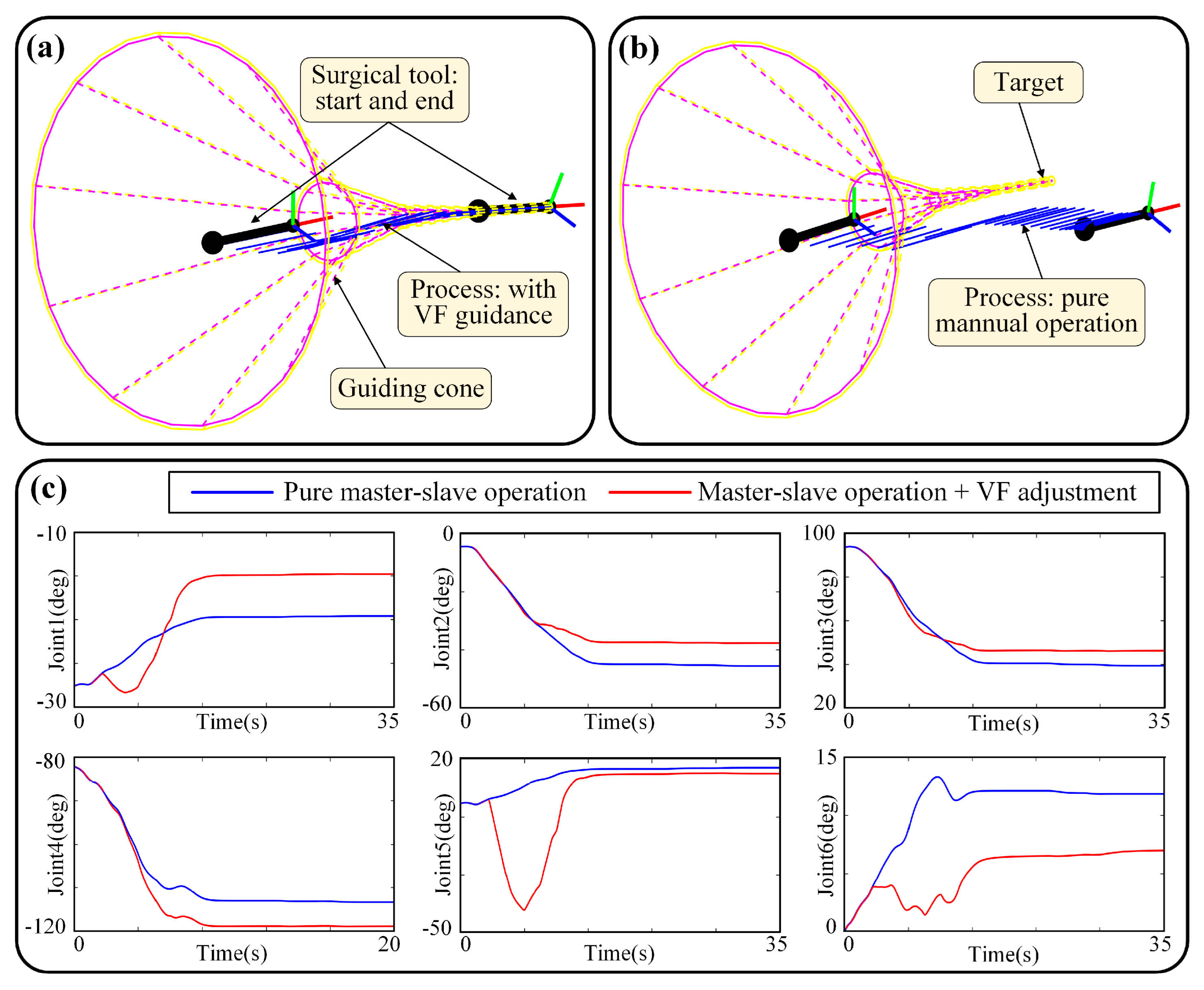
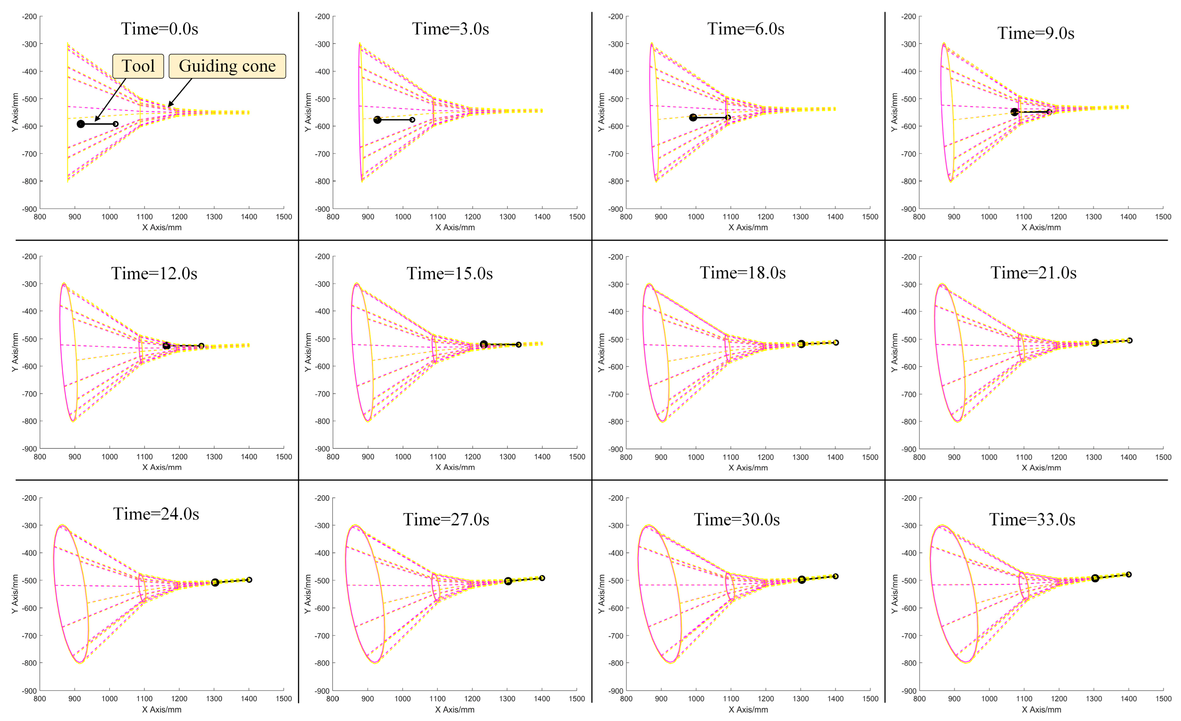
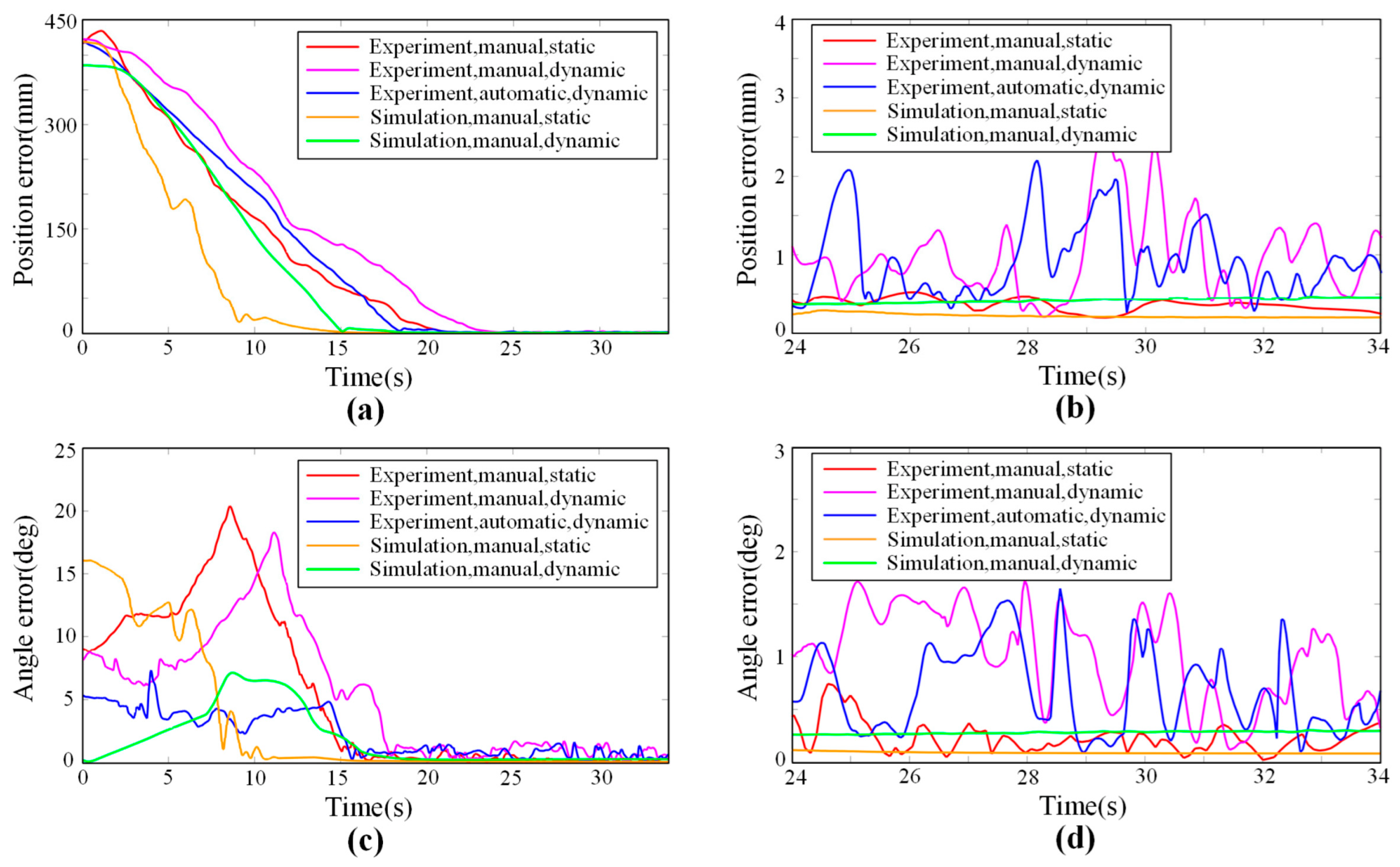
• Simulations and experiments are carried out in the work, the targets are reached, and the errors are quantitatively estimated. In simulations, the estimated positioning errors are 0.202 mm and 0.082 deg for a static target, and 0.439 mm and 0.289 deg for a dynamic target, representing the theoretical ability of VF to adjust the surgical tool. In experiments, the estimated positioning errors are 0.366 mm and 0.227 deg for a static target and 0.977 mm and 1.017 deg for a dynamic target. Despite a few errors, the results suggest the effectiveness of the proposed VF and the motion strategy, which can help the operator keep a relatively high level of accuracy during the manipulating process.
• Safety, accuracy, and dynamic adaptability are three features of the proposed method, making it a palatable auxiliary framework to assist oral surgery operations.

In the future, the motion error will be further studied with the help of precision measurement in order to archive better accuracy. Additionally, force sensing and force feedback methods will be introduced into the current framework to further improve the performance. In addition, the programming of this work will be integrated into a 3D-visualization software for the oral surgical robot system to make it more convenient.

References

- Shanti, R.M.; O’Malley, B.W. Surgical Management of Oral Cancer. Dent. Clin. N. Am. 2018, 62, 77–86. [Google Scholar] [CrossRef] [PubMed]
- Johnston, L.; Warrilow, L.; Fullwood, I.; Tanday, A. Fifteen-minute consultation: Oral ulceration in children. Arch. Dis. Chidhood-Educ. Pract. Ed. 2021, 107, 257–264. [Google Scholar] [CrossRef] [PubMed]
- Carvalho, R.; Botelho, J.; Machado, V.; Mascarenhas, P.; Alcoforado, G.; Mendes, J.; Chambrone, L. Predictors of tooth loss during long-term periodontal maintenance: An updated systematic review. J. Clin. Periodontol. 2021, 48, 1019–1036. [Google Scholar] [CrossRef] [PubMed]
- Kudsi, Z.; Fenlon, M.; Johal, A.; Baysan, A. Assessment of Psychological Disturbance in Patients with Tooth Loss: A Systematic Review of Assessment Tools. J. Prosthodont. Implant Esthet. Reconstr. Dent. 2020, 29, 193–200. [Google Scholar] [CrossRef] [PubMed]
- Hosadurga, R.; Soe, H.; Lim, A.; Adl, A.; Mathew, M. Association between tooth loss and hypertension: A cross-sectional study. J. Fam. Med. Prim. Care 2020, 9, 925–932. [Google Scholar] [CrossRef]
- McMahon, J.; Steele, P.; Kyzas, P.; Pollard, C.; Jampana, R.; MacIver, C.; Subramaniam, S.; Devine, J.; Wales, C.; McCaul, J. Operative tactics in floor of mouth and tongue cancer resection—The importance of imaging and planning. Br. J. Oral Maxillofac. Surg. 2021, 59, 5–15. [Google Scholar] [CrossRef]
- Flanagan, D. Rationale for Mini Dental Implant Treatment. J. Oral Implantol. 2021, 47, 437–444. [Google Scholar] [CrossRef]
- Hupp, J. Robotics and Oral-Maxillofacial Surgery. J. Oral Maxillofac. Surg. 2020, 78, 493–495. [Google Scholar] [CrossRef]
- Yee, S. Transoral Robotic Surgery. Aorn J. 2017, 105, 73–81. [Google Scholar] [CrossRef]
- Ahmad, P.; Alam, M.K.; Aldajani, A.; Alahmari, A.; Alanazi, A.; Stoddart, M.; Sghaireen, M.G. Dental Robotics: A Disruptive Technology. Sensors 2021, 21, 3308. [Google Scholar] [CrossRef]
- Zhang, J.; Wang, W.; Cai, Y.; Li, J.; Zeng, Y.; Chen, L.; Yuan, F.; Ji, Z.; Wang, Y.; Wyrwa, J. A Novel Single-Arm Stapling Robot for Oral and Maxillofacial Surgery-Design and Verification. IEEE Robot. Autom. Lett. 2022, 7, 1348–1355. [Google Scholar] [CrossRef]
- Yuan, F.; Liang., S.; Lyu., P. A Novel Method for Adjusting the Taper and Adaption of Automatic Tooth Preparations with a High-Power Femtosecond Laser. J. Clin. Med. 2021, 10, 3389. [Google Scholar] [CrossRef]
- Gao, Z.; Zhu, M.; Yu, J. A Novel Camera Calibration Pattern Robust to Incomplete Pattern Projection. IEEE Sens. J. 2021, 21, 10051–10060. [Google Scholar] [CrossRef]
- Veras, L.; Medeiros, F.; Guimaraes, L. Rapidly exploring Random Tree* with a sampling method based on Sukharev grids and convex vertices of safety hulls of obstacles. Int. J. Adv. Robot. Syst. 2019, 16, 1729881419825941. [Google Scholar] [CrossRef]
- Machmudah, A.; Parman, S.; Zainuddin, A.; Chacko, S. Polynomial joint angle arm robot motion planning in complex geometrical obstacles. Appl. Soft Comput. 2013, 13, 1099–1109. [Google Scholar] [CrossRef]
- Kim, J.H.; Kim, K.B.; Kim, S.H.; Kim, W.C.; Kim., H.Y.; Kim, J.H. Quantitative evaluation of common errors in digital impression obtained by using an LED blue light in-office CAD/CAM system. Quintessence Int. 2015, 46, 401–407. [Google Scholar] [CrossRef]
- Chen, Z.; Su, W.; Li, B.; Deng, B.; Wu, H.; Liu, B. An intermediate point obstacle avoidance algorithm for serial robot. Adv. Mech. Eng. 2018, 10, 1687814018774627. [Google Scholar] [CrossRef]
- Ma, Q.; Kobayashi, E.; Suenaga, H.; Hara, K.; Wang, J.; Nakagawa, K.; Sakuma, I.; Masamune, K. Autonomous Surgical Robot With Camera-Based Markerless Navigation for Oral and Maxillofacial Surgery. IEEE-ASME Trans. Mechatron. 2020, 25, 1084–1094. [Google Scholar] [CrossRef]
- Hu, Y.; Li, J.; Chen, Y.; Wang, Q.; Chi, C.; Zhang, H.; Gao, Q.; Lan, Y.; Li, Z.; Mu, Z.; et al. Design and Control of a Highly Redundant Rigid-flexible Coupling Robot to Assist the COVID-19 Oropharyngeal-Swab Sampling. IEEE Robot. Autom. Lett. 2022, 7, 1856–1863. [Google Scholar] [CrossRef]
- Cheng, K.; Kan, T.; Liu, Y.; Zhu, W.; Zhu, F.; Wang, W.; Jiang, X.; Dong, X. Accuracy of dental implant surgery with robotic position feedback and registration algorithm: An in-vitro study. Comput. Biol. Med. 2021, 129, 104153. [Google Scholar] [CrossRef]
- Toosi, A.; Arbabtafti, M.; Richardson, B. Virtual Reality Haptic Simulation of Root Canal Therapy. Appl. Mech. Mater. 2014, 66, 388–392. [Google Scholar] [CrossRef]
- Kasahara, Y.; Kawana, H.; Usuda, S.; Ohnishi, K. Telerobotic-assisted bone-drilling system using bilateral control with feed operation scaling and cutting force scaling. Int. J. Med. Robot. Comput. Assist. Surg. 2012, 8, 221–229. [Google Scholar] [CrossRef] [PubMed]
- Iijima, T.; Matsunaga, T.; Shimono, T.; Ohnishi, K.; Usuda, S.; Kawana, H. Development of a Multi DOF Haptic Robot for Dentistry and Oral Surgery. In Proceedings of the 2020 IEEE/SICE International Symposium on System Integration, Honolulu, HI, USA, 12–15 January 2020; pp. 52–57. [Google Scholar]
- Li, J.; Lam, W.; Hsung, R.; Pow, E.; Wu, C.; Wang, Z. Control and Motion Scaling of a Compact Cable-driven Dental Robotic Manipulator. In Proceedings of the 2019 IEEE/ASME International Conference on Advanced Intelligent Mechatronics, Hong Kong, China, 8–12 July 2019; pp. 1002–1007. [Google Scholar]
- Kwon, Y.; Tae, K.; Yi, B. Suspension laryngoscopy using a curved-frame trans-oral robotic system. Int. J. Comput. Assist. Radiol. Surg. 2014, 9, 535–540. [Google Scholar] [CrossRef] [PubMed]
- Rosenberg, L. Virtual fixtures: Perceptual tools for telerobotic manipulation. In Proceedings of the IEEE Virtual Reality Annual International Symposium, Seattle, WA, USA, 18–22 September 1993; pp. 76–82. [Google Scholar]
- Abbott, J.; Marayong, P.; Okamura, A. Haptic virtual fixtures for robot-assisted manipulation. In Proceedings of the 12th International Symposium on Robotics Research, San Francisco, CA, USA, 12–15 October 2005; pp. 49–64. [Google Scholar]
- Abbott, J.; Okamura, A. Stable forbidden-region virtual fixtures for bilateral telemanipulation. J. Dyn. Syst. Meas. Control-Trans. ASME 2006, 128, 53–64. [Google Scholar] [CrossRef]
- Bettini, A.; Marayong, P.; Lang, S.; Okamura, A.; Hager, G. Vision-assisted control for manipulation using virtual fixtures. IEEE Trans. Robot. Autom. 2004, 20, 953–966. [Google Scholar] [CrossRef]
- Abbott, J.; Okamura, A. Pseudo-admittance bilateral telemanipulation with guidance virtual fixtures. Int. J. Robot. Res. 2007, 26, 865–884. [Google Scholar] [CrossRef]
- Kikuuwe, R.; Takesue, N.; Fujimoto, H. A control framework to generate nonenergy-storing virtual fixtures: Use of simulated plasticity. IEEE Trans. Robot. 2008, 24, 781–793. [Google Scholar] [CrossRef]
- Lin, A.; Tang, Y.; Gan, M.; Huang, L.; Kuang, S.; Sun, L. A Virtual Fixtures Control Method of Surgical Robot Based on Human Arm Kinematics Model. IEEE Access 2019, 7, 135656–135664. [Google Scholar] [CrossRef]
- Bazzi, D.; Roveda, F.; Zanchettin, A.; Rocco, P. A Unified Approach for Virtual Fixtures and Goal-Driven Variable Admittance Control in Manual Guidance Applications. IEEE Robot. Autom. Lett. 2021, 6, 6378–6385. [Google Scholar] [CrossRef]
- Tang, A.; Cao, Q.; Pan, T. Spatial motion constraints for a minimally invasive surgical robot using customizable virtual fixtures. Int. J. Med. Robot. Comput. Assist. Surg. 2014, 10, 447–460. [Google Scholar] [CrossRef]
- Pruks, V.; Farkhatdinov, I.; Ryu, J. Preliminary Study on Real-Time Interactive Virtual Fixture Generation Method for Shared Teleoperation in Unstructured Environments. In Proceedings of the 11th International Conference on Haptics—Science, Technology, and Applications, Pisa, Italy, 13–16 June 2018; pp. 648–659. [Google Scholar]
- Marinho, M.; Adorno, B.; Harada, K.; Mitsuishi, M. Dynamic Active Constraints for Surgical Robots Using Vector-Field Inequalities. IEEE Trans. Robot. 2019, 35, 1166–1185. [Google Scholar] [CrossRef]
- Xu, C.; Lin, L.; Aung, Z.; Chai, G.; Xie, L. Research on spatial motion safety constraints and cooperative control of robot-assisted craniotomy: Beagle model experiment verification. Int. J. Med. Robot. Comput. Assist. Surg. 2021, 17, e2231. [Google Scholar] [CrossRef]
- Li, M.; Ishii, M.; Taylor, R. Spatial Motion Constraints Using Virtual Fixtures Generated by Anatomy. IEEE Trans. Robot. 2007, 17, 4–19. [Google Scholar] [CrossRef]
- Ren, J.; Patel, R.; McIsaac, K.; Guiraudon, G.; Peters, T. Dynamic 3-D virtual fixtures for minimally invasive beating heart procedures. IEEE Trans. Med. Imaging 2008, 27, 1061–1070. [Google Scholar] [CrossRef]
- He, C.; Yang, E.; McIsaac, K.; Patel, N.; Ebrahimi, A.; Shahbazi, M.; Gehlbach, P.; Iordachita, I. Automatic Light Pipe Actuating System for Bimanual Robot-Assisted Retinal Surgery. IEEE Trans. Mechatron. 2020, 25, 2846–2857. [Google Scholar] [CrossRef]
- Valdenebro, A. Visualizing rotations and composition of rotations with the Rodrigues vector. Eur. J. Phys. 2016, 37, 065001. [Google Scholar] [CrossRef]
- Shi, H.; Liu, Q.; Mei, X. Visualizing rotations and composition of rotations with the Rodrigues vector. Machines 2021, 9, 213. [Google Scholar] [CrossRef]