Abstract
To obtain high-resolution and high-precision images, the aviation remote sensing stabilization platform (ARSSP) is used, which enables the isolation of unpredictable aerial camera movements during aerial photography. However, because of the interaxle coupling interference and other nonlinear interferences in the ARSSP system, the imaging quality of the aerial camera is adversely affected. Therefore, we derived the dynamic model of moment coupling between shafts to illustrate the problem. On the basis of the former proportion integration differentiation (PID) controller based on cerebellar neural network, a nonlinear cross feedback decoupling scheme is adopted to reduce the adverse effects of these interferences. The cerebellar model articulation controller (CMAC) based on synovial membrane control (SMC) is used to reduce the nonlinear interferences caused by the new cross-decoupling module. To verify the effectiveness of the scheme, simulation, indoor and outdoor experiments were conducted. The results showed that the SMC-CMAC significantly reduced the interaxle coupling effect and effectively suppressed the nonlinear interference, resulting in a good tracking performance of the ARSSP system.
1. Introduction
The aviation remote sensing stabilization platform (ARSSP) is widely used in airborne aerial remote sensing systems. The main components of a typical aerial remote sensing system include a large field-of-view push-broom charge coupled device aerial camera, ARSSP, and a position & orientation system [1]. Changes in the attitude of the aircraft caused by airflow, vibration, and other factors affect the visual axis of the aerial camera, causing overlap and distortion in aerial photographs [2,3]. Therefore, the ARSSP can be used to eliminate high-frequency interference over a wide range, while improving the accuracy and stability of the visual axis of the aerial camera. However, due to the transmission chain and friction, coupling and nonlinear interferences will inevitably occur in the process of the line-of-sight tracking of ARSSP. Hongjun [4] used Euler equations for dynamic modeling, enriched the system dynamics model through parameter identification, and deduced the nonlinear feedback control rate of the ARSSP controller. To effectively reduce interaxle coupling, a nonlinear feedback decoupling control scheme based on the Lyapunov function was proposed. In a previous study, the mathematical model of the ARSSP was analyzed, accurate coupling terms were obtained, and feedforward compensation was applied to weaken the coupling effect of the ARSSP system, which reduced the yaw axis error by 40% [5]. Moreover, adaptive decoupling control based on a neural network, which uses the principle of Lie derivative decoupling to perform a full-state linearization of the coupled system, followed by linear feedback, was proposed [6]. Simultaneously, the neural network compensates for possible uncertainties in the control system. A cerebellar model joint controller was proposed to recognize and control complex dynamic systems, such as the ARSSP system [7]. However, the output of the cerebellar model articulation controller (CMAC) was discrete, which caused the system control action to vibrate. The radial basis function neural network controller was used to approximate the unknown nonlinear disturbance of the ARSSP system [8]; however, the learning speed of the control was slow, which greatly affected the control efficiency of the system. Furthermore, the researchers proposed credit allocation (CA) to solve the shortcomings of the CMAC output curve, which is not smooth enough and has a constant weight [9]. However, the CMAC adopts a proportional-integral-derivative (PID) control algorithm, readily causing integral saturation and overshoot [10]. If , then is the edge point, and is the edge image of the gradient operator, also known as the edge intensity.
In this study, we established a dynamic model of the ARSSP system, analyzed interaxle coupling and nonlinear interference, employed a nonlinear cross-feedback decoupling scheme to reduce the interaxle coupling interference, and used a sliding-mode CMAC controller to reduce the nonlinear interference so that the ARSSP system could maintain excellent optical pointing precision stability while moving [11]. The experimental results showed that the optical pointing precision and stability of the ARSSP system were significantly improved.
2. ARSSP Dynamic Modeling
The ARSSP mainly consists of three shaft frames and a platform base. The three frames are the pitch frame, roll frame, and azimuth frame. Since the range of motion of the three frames is relatively small, the torque required is relatively large, and gears are used to reduce the size and weight of the actuator while increasing the torque of the brushless torque motor. Because the brushless torque motor is driven by gears, the azimuth frame is installed on the pitch frame, and the pitch frame is installed on the roll frame to facilitate the modeling and analysis of the ARSSP. The roll frame is installed on the ARSSP base. To measure the three inertial angular velocities and positions, each frame axis is equipped with a gyroscope and a photoelectric encoder, respectively. Figure 1 shows the principal diagram of the ARSSP.
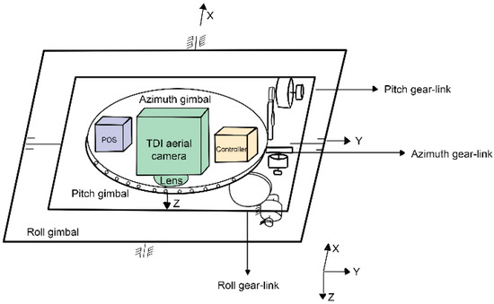
Figure 1.
Principal diagram of the ARSSP.
Figure 2 shows a three-dimensional view of the ARSSP and gear drive system. The specific parameters are as follows: rolling frame motion in the range of −10°–+10°, pitch frame movement in the range of −10°–+10°, azimuth frame movement in the range of −30°–+30°, working temperature in the range of −20 °C–+55 °C, relative humidity in the range of 95 ± 3%, load capacity ≤ 6 kg, and platform weight ≤ 3.5 kg. When the effect of the gear backlash is ignored, the gear drive system can be simplified by fixing the transmission ratio.
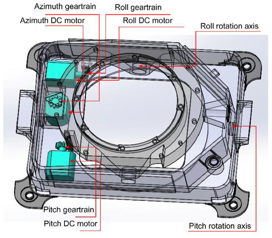
Figure 2.
Three-dimensional structure of the ARSSP.
2.1. Coordinate System
The dynamic modeling and analysis of the ARSSP system were conducted by setting the ARSSP base coordinate system , roll frame coordinate system , pitch frame coordinate system , and azimuth frame coordinate system [12]. The roll frame axis rotates around the base axis at a relative angle of , and the corresponding transformation matrix is . The pitch frame axis rotates around the roll frame axis by a relative angle of , and the corresponding transformation matrix is . The azimuth frame axis rotates around the pitch frame axis by a relative angle of , and the corresponding transformation matrix is . Figure 3 shows the specific coordinate system.
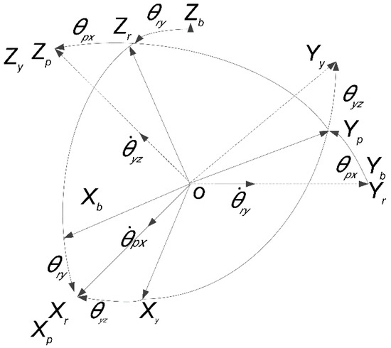
Figure 3.
Rotation of the azimuth axis by around the pitch axis.
The transformation matrix corresponding to the coordinate system shown in Figure 3 is as follows:
Set the absolute angular velocity of each frame rotation axis as , , and . The angular velocity components of the roll axis in the inertial space are , , and . According to the relative angular velocities and reference angular velocities of the ARSSP, the kinematic formulas of the angular velocities of the three rotating shaft frames are as follows: the angular velocities of the roll axis around the three axes are described as
the angular velocities of the pitch axis around the three axes are described as
and the angular velocities of the azimuth axis around the three axes are described as
According to Equations (1)–(4), the angular velocities of the ARSSP around the three-axis frame are as follows:
2.2. Coupling Analysis of the ARSSP
In the ARSSP, the torque is produced by a brushless direct current (DC) torque motor. The driving torque should be sufficient to suppress interference. Simultaneously, to reduce nonlinear interference, we made the frame of the ARSSP symmetric. The main diagonal of the inertia matrix is not zero, whereas its nonmain diagonal is zero. According to the Newton–Euler rotation equation, the torques of the three axes are as follows:
Therefore, for the torque equation of the roll axis, the moment of the roll axis is , defined as follows:
For the torque equation of the pitch axis, the pitch axis moment is , defined as follows:
For the torque equation of the azimuth axis, the azimuth axis torque is , defined as follows:
By combining Equations (7)–(9), we can obtain the moment equation of the ARSSP as follows:
Finally, Equation (10) is expanded, and the following expression is obtained:
Equation (11) is further processed to obtain the following equation:
In Equation (12), there is a coupling term that mainly consists of two parts: the interaxle coupling and the coupling moment between the base and each axis. The interaxle coupling includes , , and , which represent the coupling moments of the pitch, roll, and azimuth axes, respectively. Among them, the coupling moments include , , and , which represent the coupling moments between the pitch axis and the base, between the roll axis and the base, and between the azimuth axis and the base, respectively. For the pitch axis, the coupling torque between the pitch axis and other axes is as follows:
Among them, the coupling moment of the base is mainly between the pitch axis and the base, and the specific formula is as follows:
For the roll axis, the coupling torque between the roll axis and other axes is as follows:
Among them, the coupling torque of the base is mainly between the roll axis and the base, and the specific formula is as follows:
For the azimuth axis, the coupling torque between the azimuth axis and other axes is as follows:
Among them, the coupling torque of the base is mainly between the azimuth axis and the base, and the specific formula is as follows:
2.3. Mathematical Model of the ARSSP
The brushless DC torque motor of the ARSSP generates torque to rotate the frame. Figure 4 shows the schematic diagram of the brushless DC torque motor.

Figure 4.
Schematic diagram of the brushless DC torque motor.
According to the voltage balance equation and motor torque equation [7], we can finally obtain the torque equation of single shaft motor as follows:
where is the moment of inertia between the load and frame, is the equivalent load damping, is the armature voltage, is the resistance, is the back electromotive force coefficient, is the inductance, and is the rotational angular velocity of the brushless DC torque motor, is the torsion coefficient of the motor, and is the friction torque.
According to Equations (12) and (19), a comprehensive mathematical model of the ARSSP is derived:
To improve the accuracy of the ARSSP dynamic model, the frictional interference Stribeck curve is introduced as the main external disturbance part as follows:
When , the static friction is
When , the dynamic friction is
In Equations (21) and (22), is the driving force, is the maximum static friction force, is the Coulomb friction force, is the proportional coefficient of viscous friction torque, is the rotational angular velocity, and are constants.
3. ARSSP Controller Design
3.1. CMAC Control Algorithm
The ARSSP system is nonlinear. In the actual working process, unknown nonlinear disturbances and other factors affect the accuracy and stability of the boresight direction of the ARSSP system [13,14]. Through learning, the CMAC can approximate any linear or nonlinear mapping, making the system more robust. However, for the traditional CMAC, factors such as overlearning likely affect learning efficiency and potentially cause system collapse. The CMAC algorithm is as follows:
When the CMAC is combined with SMC, the specific formula is as follows:
For traditional CMAC weights, the gradient descent method is generally used; thus, the CMAC weight adjustment index is defined as follows:
At the end of each control cycle, the output of the CMAC is compared with the total control output , and then it is adjusted before the new learning process. The error between the total control input and the CMAC output gradually decreases until the total control input provided by the CMAC is reached. However, the traditional gradient descent method of the CMAC is prone to the phenomenon of a local optimum; thus, the weight adjustment equation of the CMAC must be improved.
3.2. CA&OS-CMAC Control Algorithm
The traditional CMAC control algorithm is prone to the phenomenon of a local optimum because of the gradient descent method, which greatly affects the learning efficiency [15]. In the traditional CMAC, the errors in the learning process are equally distributed among the activated storage units due to the same credit. Therefore, the learning efficiency and control accuracy of the traditional CMAC are reduced [16]. To improve the learning efficiency and control accuracy of the CMAC, separate storage units with different credits must be designed during the learning process. Therefore, an improved CMAC control algorithm is proposed based on CA that is suitable for the ARSSP. The concept of the CA based CMAC is as follows: First, the learning time of the storage unit is used as the basis for CA based on the update frequency of the weight of each storage unit in the CMAC. Second, the learning time for addressing the storage unit must be proportional to the reciprocal of the learning time for addressing the storage unit. Finally, the higher the credibility of the storage unit, the smaller is the amount of error correction of the system. Therefore, Equation (25) is rewritten as follows:
where is the learning efficiency of the network, i.e., the learning rate, and its value range is , and is the learning time of the th storage unit, which represents the reliability of the th storage unit. First, if , then when the th memory cell is addressed. At the end of each learning process, is automatically updated to zero. In the CMAC training process, the correction error of the memory unit activated by the neural network is proportional to .
Through this update algorithm, we can appropriately distribute the learning effect to the addressed storage unit based on the reliability of the storage unit. The in the update algorithm is used to make the denominator non-zero. To accurately adjust the credits of storage cells with different learning times, Equation (26) is revised as follows:
where represents the learning time of the th storage unit updated at the th moment, i.e., the credit of the th storage unit, and the parameter is the equilibrium constant. is updated to zero at the end of the learning process, modifying equation (27) from −1 to . Therefore, as the storage units of the learning algorithm and the stored content increase, the credibility improves and the amount of error correction reduces. Therefore, a reasonable balance constant can effectively improve the learning speed of CMAC in early learning. When the ARSSP is applied to different camera loads, the balance constant needs to be adjusted according to the actual process to optimize the learning process. Therefore, the CA based CMAC algorithm enables the storage unit with less learning time to have a smaller credit and correction with a larger weight, enhancing the accuracy and stability of the CMAC control system.
The signal output by the CMAC is discrete and has low smoothness; thus, the output signal needs to be optimized. The specific design process of the CMAC algorithm for OS and the error matrix of the sliding-mode CMAC controller is as follows:
where is the total output matrix of the controller, is the output matrix of the sliding-mode CMAC controller, is the selection matrix of the activation unit, and is the matrix of the physical storage space. The matrix form of the adjusted weight equation of the conventional CMAC can be rewritten as follows:
where , and when combined with Equations (14) and (15), the following weight update formula can be obtained:
According to the idea that the adjacent weight change value in the CMAC is the smallest, the ideal result is to achieve a smaller output error while smoothing the output waveform. For the traditional CMAC, the least mean square algorithm (LMS) is usually used in weight adjustment. The LMS algorithm mainly adjusts the weight of each storage unit in each learning process according to the minimum value of the output error, which can quickly reduce the output error of the CMAC but introduces the problem of output mutation. Therefore, for the CMAC control algorithm that optimizes the smoothness, it is feasible to simultaneously reduce the output error and smoothen the adjacent weight change so that the output of the sliding-mode CMAC controller can be smoothened. However, the sliding-mode CMAC controller with OS has an extended stability time. Therefore, to improve the stability time and smoothness accuracy of the system, the smoothing parameter is used for adjustment. The weight adjustment formula of the OS-CMAC is as follows:
Finally, the compound CMAC algorithm based on CA and OS is as follows:
3.3. Design of the Sliding-Mode Controller Based on the CMAC
The ARSSP system can be described as a multi-input, multi-output, nonlinear uncertain system. The SMC controller is designed to reduce the nonlinear interference and ensure the robustness and stability of the system. The system state space model is as follows:
where is the control input , is the system state vector, is the uncertain interference term, is the output vector, and is the friction interference term. We make the following assumptions:
Hypothesis 1:
The system output has a range, and the derivative has a range.
Hypothesis 2:
During the movement of the ARSSP, we ignore the interaxis coupling interference term and other nonlinear interference terms because of the limited range of motion.
The ideal control signal is , where the error signal is , and the sliding model we obtain is as follows:
where is a constant. According to the linear feedback theory, the sliding-mode control rate is as follows:
where is the switching gain coefficient, and . The Lyapunov function is defined as
Combining Equations (14)–(16), Lyapunov’s derivative becomes
Chattering is strong because of the huge change in the switching gain coefficient . To eliminate chattering, the saturation function is used instead of .
Based on the compound CMAC algorithm, which involves CA and OS, the sliding-mode CMAC control rate is designed by combining both the SMC controller and Equation (35) as follows:
The sliding-mode CMAC controller is used as the torque control unit; the cross-feedback decoupling scheme is used as the main coupling interference unit; the Stribeck friction curve is used as the friction compensation unit; the compound algorithm based on CA and OS is used as the CMAC optimization unit. The structural diagram of the ARSSP system shown in Figure 5 is designed to facilitate understanding. According to this diagram, the system is mainly composed of three parts: First, the torque motor control module consists of the sliding-mode CMAC controller and the CMAC optimization unit. The control voltage of the torque motor is the control input for driving the three rotating shaft frames. Second, the coupling compensation module mainly consists of the compensation module for base coupling and the compensation module for the coupling of each frame. Among these modules, the cross-feedback module is involved in base coupling, and each frame axis module couples the feedback compensation control system. Given that the shaft frame contains a feedback signal, which mainly includes angular position, angular velocity, and angular acceleration, the control input of the coupling item is the feedback signal of the shaft frame, which can achieve closed-loop ARSSP control. In this way, the posture stability of the three rotating shaft frames is maintained in a balanced state. Third, based on the calculated compensation items for the coupling torque of the base and interaxle coupling, the cross-feedback module allocates compensation items to different control channels of the three-axis ARSSP. The attitude stability of the ARSSP can be improved by employing the cross-feedback compensation module to compensate for the coupling torque of the base and the coupling torque of the shaft frame.
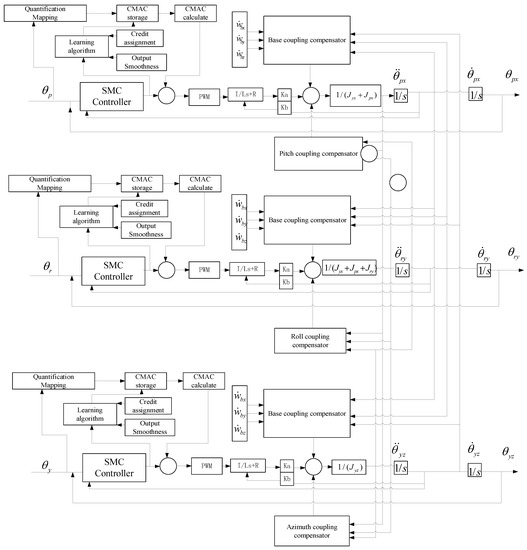
Figure 5.
Structural diagram of the ARSSP control system.
4. Experimental Analysis
4.1. Simulation Experiment
To evaluate the effectiveness of the sliding-mode compound CMAC algorithm based on CA and OS, simulations were performed. In the ARSSP, the pitch axis frame is more susceptible to interference torque than the other two-axis frames; thus, in this study, the pitch gimbal system was selected as the analysis object. The reference input-angle signal of each axis is shown in Figure 6. The pitch axis input is a step signal with a step value of 0.25 s, and the final value is 1°. The input signal of the roll shaft is a step signal during 0–1 s and a sine signal, given by , during 1–2 s; the step value is 0.5 s and the final value is 2°. The expression is . The input signal of yaw axis is 0 during the period 0–1.5 s and a sine signal during the period 1.5–2 s; the expression is . The CMAC controller parameters were as follows: , , , , a period of 1.0, and a sampling period of 0.001 s. The sliding-mode controller parameters were and . The saturation parameters were The mathematical model parameters were as follows: ; gear ratio ; and resistance . The moment of inertia parameters were as follows: .
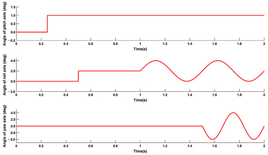
Figure 6.
Reference input–angle signal of each axis.
The goal of the simulation experiment was to use the traditional CMAC + PID controller for comparative analysis. Figure 7, Figure 8 and Figure 9 show the experimental results.
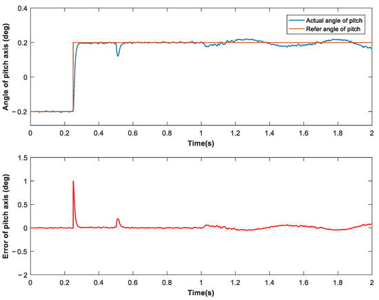
Figure 7.
Response of pitch axis under CMAC–PID control.
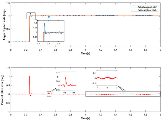
Figure 8.
Response of pitch axis with cross-feedback module under CMAC–PID control.
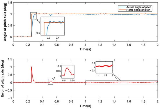
Figure 9.
Response of pitch axis with cross-feedback module under CMAC-SMC control.
According to the experimental results, traditional CMAC–PID control can effectively control overshoot and resist static impact interference. However, it fails to deal with dynamic disturbance such as the coupling torque between shafts. After introducing cross-feedback decoupling structure, CMAC–PID controller can deal with dynamic disturbance. However, it can be seen from the simulation results that its dynamic performance has deteriorated. This may be attributed to the introduction of new modules that have changed the nonlinearity of the system. According to Figure 9, the sliding-mode controller using the composite CMAC algorithm of the cross-decoupling scheme provides strong output signal stability. The introduction of SMC obviously suppresses overshoot and has performs well in dealing with static impact and dynamic disturbances.
4.2. Experimental Verification
To evaluate the effectiveness of the cross-feedback decoupling control, it is necessary to conduct a comparative analysis of the optical pointing precision error before and after system decoupling. Figure 10 shows the optical pointing precision error using a two-axis simulation test bench, NORMAT5000 two-axis photoelectric autocollimator, ARSSP, plane mirror, adjustable bracket, laser aligner, and other components. The specific process was to use the two-axis simulation test bench to simulate the attitude of the aircraft movement, so that the ARSSP can obtain and compensate the attitude angle, and use the NORMAT5000 dual-axis photoelectric autocollimator and the plane mirror to obtain the optical pointing precision error before and after the ARSSP attitude compensation.
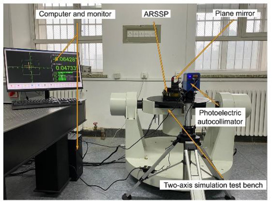
Figure 10.
Indoor test site.
The specific requirements of the experimental test indicators are the viewing axis pointing accuracy error experimental angle range from −5 to 5 (deg) and the angular position tracking experimental angle range from 0 to 1 (deg). Table 1 and Table 2 show the instrument parameters.

Table 1.
Main technical parameters of the two-axis simulation test bench.

Table 2.
Main technical parameters of the dual-axis photoelectric autocollimator.
The specific experimental process was as follows: the rotation angle of the two-axis simulation test bench was β, the ARSSP rotated β, and then, angle compensation was performed. The compensation angle was β’, and the boresight pointing accuracy error was the difference between β’and β. Figure 11 shows the schematic diagram of the experimental process.
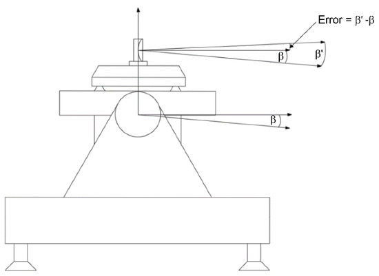
Figure 11.
Schematic diagram of the experimental process.
Through the optical pointing precision error experiment, the actual error data before and after decoupling were obtained. After comparing the error data, the effectiveness of the cross-feedback decoupling control was verified. Figure 12, Figure 13, Figure 14 and Figure 15 show the experimental results.
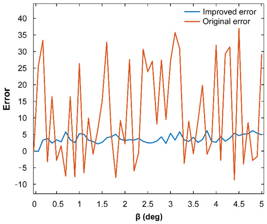
Figure 12.
Precision error curve of the pitch axis boresight pointing.
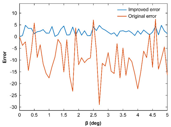
Figure 13.
Precision error curve of the roll axis boresight pointing.
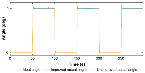
Figure 14.
Pitch axis decoupling front and rear angular position tracking curve.
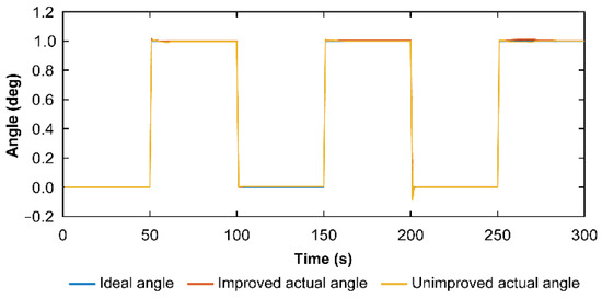
Figure 15.
Roll axis decoupling front and rear angular position tracking curve.
According to the experimental results, the use of cross-feedback decoupling control can effectively reduce the influence of the coupling torque on the pointing accuracy of the system’s boresight and significantly reduce the optical pointing precision error.
To further evaluate the effectiveness of the scheme, aerial cameras and aerial remote sensing stabilization platforms were used to conduct physical shooting experiments outdoors, as shown in Figure 16.
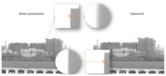
Figure 16.
Comparison results of outdoor experiments.
We took 10 images before and after applying the sliding-mode compound CMAC algorithm and took a partial image of the position shown in Figure 16, as shown in Figure 17.
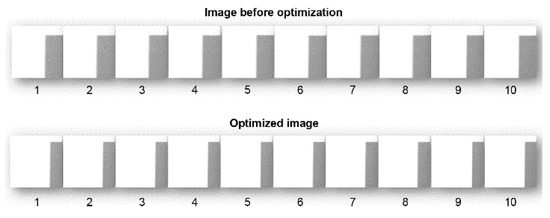
Figure 17.
Ten sets of partial images before and after optimization.
The edge strength, which is the amplitude of the edge point gradient, is an important indicator of the clarity of the image [17]. We analyzed the edge strength of the 10 groups of images to evaluate the sharpness of the images and normalized the evaluation results. Figure 18 shows the processing results.
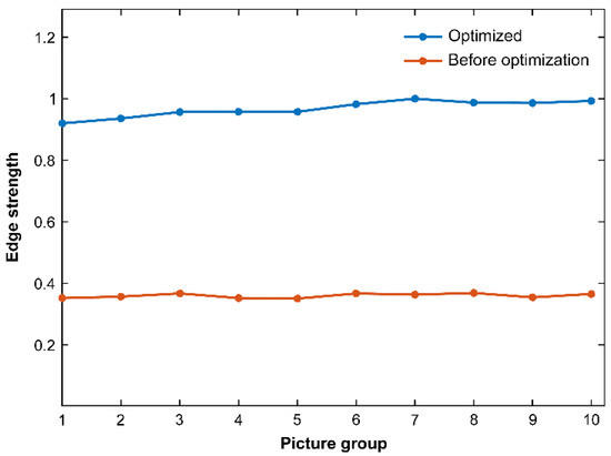
Figure 18.
Edge strength obtained from the analyzed images before and after optimization.
The analyses of the photos showed that the sharpness of the optimized photos significantly improved, confirming the improvement in the optical pointing precision and stability of the aerial remote sensing stabilization platform.
5. Conclusions
To minimize the coupling interference in the ARSSP system, we adopted a nonlinear cross-feedback decoupling scheme to compensate for the coupling terms existing in the system model. To improve the accuracy and stability of the system, the traditional cerebellar neural network PID controller was optimized based on SMC. The simulation and indoor test results showed that the proposed algorithm is effective in improving the control accuracy and stability of the platform. By performing outdoor experiments, the effectiveness of the control algorithm was indirectly verified by comparing the definitions of photographed samples.
Author Contributions
Conceptualization, T.R. and G.S.; methodology, T.R.; software, L.M.; validation, T.R., G.S. and J.L.; formal analysis, T.R.; investigation, L.M.; resources, J.L.; data curation, L.M.; writing—original draft preparation, T.R.; writing—review and editing, G.S.; visualization, L.M.; supervision, G.S.; project administration, T.R.; funding acquisition, T.R. All authors have read and agreed to the published version of the manuscript.
Funding
This research was financially supported by the Science and Technology Development Key Projects of Jilin Province (20210203024SF).
Data Availability Statement
Not applicable.
Acknowledgments
The authors would like to thank Key Laboratory of Micro-Nano and Ultra-Precision Manufacturing of Jilin Province (NO. 20140622008JC) for helpful experimental equipment related to this work.
Conflicts of Interest
The authors declare no conflict of interest.
References
- Bagheri, N. Development of a high-resolution aerial remote-sensing system for precision agriculture. Int. J. Remote Sens. 2017, 38, 2053–2065. [Google Scholar] [CrossRef]
- Xiu, J.; Zhai, L. Main factors affecting the quality of aerial images. Infrared 2005, 8, 10–16. [Google Scholar]
- Hu, J.; Zhi, X.; Gong, J.; Yin, Z.; Fan, Z. Error tolerance and effects analysis of satellite vibration characteristics and measurement error on TDICCD image restoration. Infrared Phys. Technol. 2018, 93, 277–285. [Google Scholar] [CrossRef]
- Yu, H. Decoupling and Control of Three-Axis Turntable; Harbin Institute of Technology: Shenzhen, China, 2013. [Google Scholar]
- Cunhai, L.; Guangfeng, C. Decoupling and control of three-axis turret based on modified repetitive control system. Electro-Opt. Technol. Appl. 2014, 5, 29. [Google Scholar]
- Wei, W. The Research of Optical Axis Stabilization of the Airborne Photoelectric Platform. Doctoral Dissertation, Changchun Institute of Optics, Fine Mechanics and Physics, Changchun, China, 2015. [Google Scholar]
- Zhou, X.; Li, Y.; Yue, H.; Jia, Y.; Zhao, L.; Zhu, Z. An Improved cerebellar model articulation controller based on the compound algorithms of credit assignment and optimized smoothness for a three-axis inertially stabilized platform. Mechatronics 2018, 53, 95–108. [Google Scholar] [CrossRef]
- Zeng, D. Research on the Control System of Inertially Stabilized Platform Gimbal for Airborne Remote Sensing; National University of Defense Technology: Changsha, China, 2016; pp. 1–102. [Google Scholar]
- Su, S.F.; Tao, T.; Hung, T.H. Credit assigned CMAC and its application to online learning robust controllers. IEEE Trans. Syst. Man Cybern. Part B Cybern. 2003, 33, 202–213. [Google Scholar] [CrossRef]
- Hwang, M.; Chen, Y.J.; Ju, M.Y.; Jiang, W. A fuzzy CMAC learning approach to image based visual servoing system. Inf. Sci. 2021, 576, 187–203. [Google Scholar] [CrossRef]
- Jalilzadeh, A.; Nedić, A.; Shanbhag, U.V.; Yousefian, F. A variable sample-size stochastic quasi-newton method for smooth and nonsmooth stochastic convex optimization. Math. Oper. Res. 2022, 47, 690–719. [Google Scholar] [CrossRef]
- Wang, Z. Research on Control Algorithm of Aerial Remote Sensing Stabilization Platform; Changchun University of Technology: Changchun, China, 2021. [Google Scholar]
- Zhu, Q. Complete model-free sliding mode control (CMFSMC). Sci. Rep. 2021, 11, 22565. [Google Scholar] [CrossRef] [PubMed]
- Li, Y.; Zhu, Q.; Zhang, J. Distributed adaptive fixed-time neural networks control for nonaffine nonlinear multiagent systems. Sci. Rep. 2022, 12, 8459. [Google Scholar] [CrossRef] [PubMed]
- Su, H.J.; Li, D.M.; Wang, S.L.; Zhang, Y.T.; Guo, X. Research on electron beam center trajectory correction algorithm based on differential evolution CMAC. At. Energy Sci. Technol. 2015, 49, 130–133. [Google Scholar]
- Su, G.; Chen, Z.; Yuan, Z. The theory and application of cmac. Chin. J. Sci. Instrum. 2003, 024, 269–273. [Google Scholar]
- Lindeberg, T. Edge detection and ridge detection with automatic scale selection. Int. J. Comput. Vis. 1998, 30, 117–156. [Google Scholar] [CrossRef]
Disclaimer/Publisher’s Note: The statements, opinions and data contained in all publications are solely those of the individual author(s) and contributor(s) and not of MDPI and/or the editor(s). MDPI and/or the editor(s) disclaim responsibility for any injury to people or property resulting from any ideas, methods, instructions or products referred to in the content. |
© 2022 by the authors. Licensee MDPI, Basel, Switzerland. This article is an open access article distributed under the terms and conditions of the Creative Commons Attribution (CC BY) license (https://creativecommons.org/licenses/by/4.0/).