Vibration Control of Disturbed All-Clamped Plate with an Inertial Actuator Based on Cascade Active Disturbance Rejection Control

Abstract

In this paper, active disturbance rejection control (ADRC) is applied to the vibration control of the all-clamped plate structure with an inertial actuator. Knowing that modeling uncertainties, dynamic nonlinearities and multivariable couplings are often the major causes of a downgrading performance and instability, a cascade ADRC controller is, hence, utilized to mitigate the effects of these issues. The dynamics regarding the all-clamped plate structure and inertial actuator are obtained through theoretical analysis and experimental testing. Furthermore, the real-time control experimental verification is carried out on the hardware-in-the-loop platform based on the NI PCIe-6343 data acquisition card. The comparative experimental results show that the proposed cascade ADRC controller has a better vibration suppression performance, disturbance rejection performance and decoupling ability.

1. Introduction

Electrodynamic inertial actuators (shortly, inertial actuators) have been widely used in active vibration control (AVC) to meet stringent performance requirements due to their high bandwidth capabilities, large effective stroke, good control of complex periodic vibration and so on [1,2,3]. Composed of an inertial actuator and a collected accelerometer pair with a time integrator, a control unit behaves as a configuration of a ‘virtual’ skyhook damper when direct velocity feedback (DVFB) is implemented on the device [4]. Along similar lines, control strategies can be designed to make inertial actuators act as any virtual devices based on the philosophy of virtual passive control [5]. Furthermore, the strategies of modern control theory, including optimal control, sliding mode control, nonlinear control law, etc., can be applied to inertial actuators [6,7].

In practical applications, the performance of the control method is affected by the complex dynamics of the inertial actuators, in particular, the phenomena of the phase shift below the first natural frequency of actuators, saturation and hysteresis [8]. Moreover, the control–structure interaction between the inertial actuator and the structure must necessarily be considered because ignoring it will cause the performance of the active control system to not be fully utilized, reduce the control effect or even make the system unstable [9]. In addition, the structure vibration dynamics are always uncertain and vary based on boundary conditions, installation positions of actuators, etc. [10] Therefore, various robust controllers have been proposed. In Ref. [11], an adaptive mechanism was introduced to address uncertainties. Methods based on a disturbance observer also received a lot of attention, such as the time delay estimation [12], disturbance observer [13] and extended state observer (ESO) [14].

An ESO is the core link in the frame of active disturbance rejection control (ADRC), which was first proposed by Han [15]. ADRC has became an effective tool to study nonlinear systems, and it has been rapidly popularized and applied in theoretical research, experiments and engineering [16,17,18,19]. In addition, many composite control methods combined with an ESO have been proposed, which can generally inherit the advantages of the baseline controller and ESO simultaneously. For example, a hybrid data-driven fuzzy ADRC algorithm was proposed to obtain the automatic optimal tuning in a model-free manner of the parameters in Ref. [20]. ADRC can estimate and compensate the total disturbance effect of various external disturbances and internal disturbances determined by the system’s own mechanism during operation in real time. The advantages of ADRC include fast corresponding speed, high control precision and a strong disturbance rejection ability [21]. In recent years, ADRC has also been applied in structural vibration control [22,23].

The performance of ADRC critically depends on how accurately the ESO can estimate the total disturbance [16]. The establishment principle of an ESO points out that for an n-order system, an n+1-order ESO needs to be established [24]. Unfortunately, due to the high order of the system caused by the coupling between the inertial actuator and the all-clamped plate, a high-order ESO will increase the amount of calculation and the application cost, which is not expected. Therefore, in order to establish a new model to facilitate the study, this paper studies the connection between the actuator and the structure and introduces the virtual control variable to establish the system as a cascade system composed of a series of low-order systems. The novelty of the model is two-fold: first, the concept of total disturbance is introduced under the control framework of ADRC; second, with the help of cascade control technology, the system is modeled as a cascade system to avoid the high-order observer.

In this paper, combining classical ADRC and cascade control technology, a cascade ADRC controller with low model dependence is designed based on virtual control variables to solve the multivariable and strong coupling in the vibration control based on inertial actuators. Compared with some of the previous literature, such as Refs. [4,5], etc., this is an attempt to apply advanced control theory. In addition, different from the direct application of ADRC in Ref. [8], this paper improves the control strategy according to the characteristics of structural vibration combined with cascade control in the process of application. The main advantages of the proposed controller are: (a) disturbances from inertial actuators are added to the secondary loop, which is suppressed by the inner loop; (b) the influence of the dynamics of the inertial actuator in the inner loop on the plate is greatly weakened; and (c) the response speed of the whole system is improved.

The paper is organized as follows: The dynamic characteristics of the system and the electromechanical coupling model are analyzed in Section 2. In Section 3, a cascade ADRC controller is established for the plate structure. In Section 4, experiments are carried out on the actual all-clamped plate experimental platform to verify the superiority of the method. The conclusion is indicated in Section 5.

2. Preliminaries

The dynamics regarding the all-clamped plate structure and inertial actuator will now be introduced.

2.1. Linear Dynamics of All-Clamped Plate

Based on the dynamic theory of elastic thin plates and applying modal analysis technology, the i-th vibration of plates can be constructed as follows:

$${\ddot{\eta }}_i+2{\zeta }_i{\omega }_i{\dot{\eta }}_i+{\omega }_i^2{\eta }_i=b_i{f}_{ci}+f_{di},$$

(1)

where ${\omega }_i$, ${\zeta }_i$ and ${\eta }_i$ are the natural angular frequency damping and displacement of the i-th modal, respectively, $f_{di}$ is the external modal force after conversion, $b_i$ denotes the control gain, $f_{ci}$ denotes the control force. The high-order modes are appropriately ignored, and the movement of the structure can be represented by the first n-order modal. Therefore, the transfer function between point force $f_{di}+b_i{f}_{ci}$ (input) and the displacement ${\eta }_i$ (output) can be obtained as follows [25]:

$$G_p\left(s\right)=\sum _{i=1}^n\frac{b_i}{s^2+2{\zeta }_i{\omega }_i+{\omega }_i^2}.$$

(2)

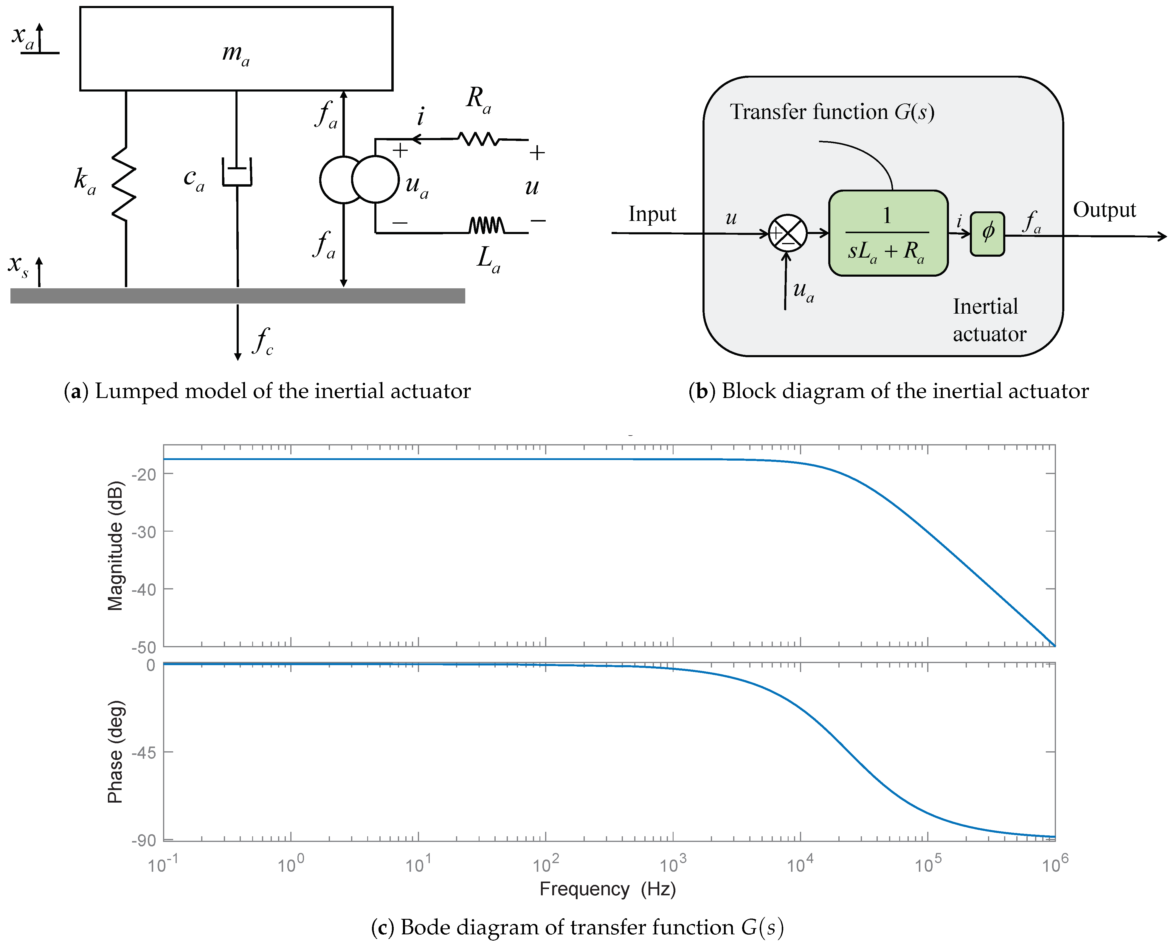
2.2. Linear Dynamics of Inertial Actuator

The schematic representation of the electrodynamic inertial actuator is shown in Figure 1a.

An electrodynamic inertial actuator is composed of a proof-mass $m_a$ attached to the base via a spring $k_a$ and damper $c_a$.

A current i is generated when a voltage u is applied across an inertial actuator. According to Lorentz’s law, the control force $f_a$ is proportional to the current i. Therefore, Equation (3) can be expressed by

$$\left\{\begin{array}{c}{f}_a=\varphi i\hfill \\ u_a=\varphi v=\varphi \left({\dot{x}}_a-{\dot{x}}_s\right)\hfill \\ u=L_e\frac{di}{dt}+R_{e}i+u_a\hfill \end{array},\right.$$

(3)

where $\varphi$ represents the transduction coefficient and $u_a$ is called the electromotive force (back-emf). The parameters of the inertial actuator used in this paper are $L_e=0.05$ mH, $R_e=7.5\Omega$ and $\varphi =7.6$. Therefore, the influence of the electromagnetic system is shown in Figure 1b. The Bode diagram of the transfer function $G\left(s\right)$ is shown in Figure 1c. It can be seen from Figure 1c that the frequency response of the electromagnetic system is flat for the interest frequency bandwidth. The actuator force $f_a$ can be considered proportional to the input voltage via a constant gain $g_a$. The electrodynamic inertial actuator can be described as a linear second-order lumped-parameter model [26]:

$$\left\{\begin{array}{c}{f}_a=g_{a}u\hfill \\ f_c=f_a+c_a({\dot{x}}_a-{\dot{x}}_s)+k_a(x_a-x_s)\hfill \\ f_c=m{\ddot{x}}_a\hfill \end{array}\right..$$

(4)

Now, the transfer function between the reaction force $f_c$ and the input voltage u can be expressed as:

$$\begin{array}{cc}\hfill F_c\left(s\right)& =\left(g_a\frac{m_a{s}^2}{m_a{s}^2+c_{a}s+k_a}\right)U\left(s\right)+\left(\frac{m_a{c}_a{s}^3+m_a{k}_a{s}^2}{m_a{s}^2+c_{a}s+k_a}\right)X_s\left(s\right)\hfill \\ \hfill & =G_{a}U\left(s\right)+G_s\left(s\right)X_s\left(s\right),\hfill \end{array}$$

(5)

in which $U\left(s\right)\mathrm{and}{X}_s\left(s\right)$ are the Laplace transform of u and $x_s$, respectively. $G_a\left(s\right)$ denotes the transfer function of the inertial actuator when its base is rigid and $G_s\left(s\right)$ represents the coupling force between, caused by structure displacement.

2.3. Nonlinear Dynamics of the System

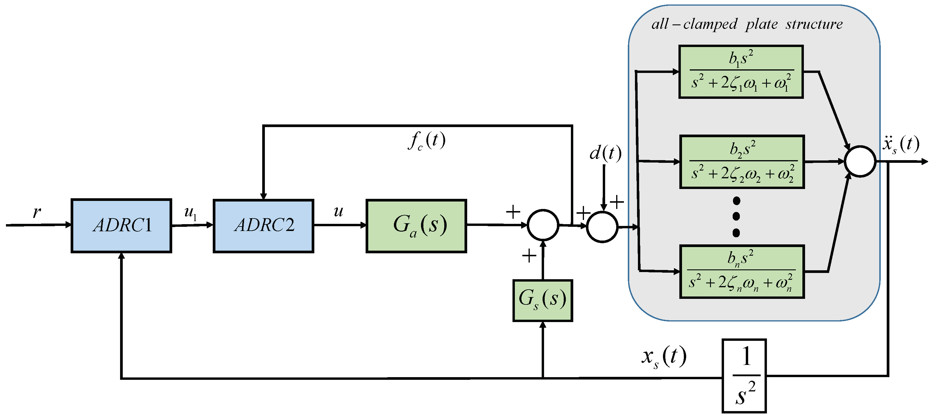
For the intractable nonlinearity existing in the system, the experimental method is applied to study it. The research method is to start from the input and output characteristics. First, the experimental device is configured as shown in Figure 2a. Because the sensor voltage has a linear relationship with the acceleration, the output force $f_c$ is, therefore, represented by sensor voltage according to Equation (4). When the signal generator applies a small sinusoidal excitation signal whose amplitude varies linearly with time, the hysteresis characteristics of the inertial actuator can be obtained as shown in Figure 2b. Then, the signal generator is still made to generate a time-varying signal, but its amplitude is amplified to a large sinusoidal excitation. The saturation phenomenon caused by the stroke of the inertial actuator can be seen in Figure 2c.

The ADRC method used in this paper is a model-free control strategy. Therefore, when studying the nonlinear characteristics of the inertial actuator, different from the existing literature, such as Ref. [9], this paper focuses not on the establishment of nonlinear models but on the display of nonlinear phenomena. The advantage of doing this is that there are few instruments required. The sensor required by the test method in this paper is only an accelerometer, and the accuracy requirements of the sensor are not high. Future work will focus on using a sensor to identify the nonlinear parameters of the actuator.

Remark 1.

Multiple sources of uncertainties in real all-clamped plate with an inertial actuator are briefly explained here. The control objective is to design the control voltage u with parameter uncertainties under the influence of the external/internal disturbances that will make structure displacement $x_s$ attenuate rapidly.

3. Control Scheme

3.1. System Re-Modeling

The displacement of the all-clamp plate $x_s={\eta }_1+{\eta }_2+\cdots +{\eta }_n$ is the controlled quantity. By taking $x_s$ as the basic state variable yields a reconstructed system model:

$${\ddot{x}}_s=-2{\zeta }_0{\omega }_0{\dot{x}}_s-{\omega }_0{x}_s+b{f}_c+w(\eta ,\dot{\eta }),$$

(6)

where $b={\displaystyle \sum _1^n}{b}_i$ denotes control gain and $w(\eta ,\dot{\eta })=-{\displaystyle \sum _1^n}\left[2\left({\zeta }_i{\omega }_i-{\zeta }_0{\omega }_0\right){\dot{x}}_i+\left({\omega }_i^2-{\omega }_0^2\right)x_i\right]$ is treated as external disturbance. In this way, the multi-modal plate structure can be simplified to a single-input single-output system. Therefore, the system can be established as a cascade form as Equation (7). The control quantity u directly drives $m_a{\ddot{x}}_a$, and $m_a{\ddot{x}}_a$ then directly drives $x_s$ to achieve the control purpose.

$$\left\{\begin{array}{c}{\ddot{x}}_s=-2{\zeta }_0{\omega }_0{\dot{x}}_s-{\omega }_0{x}_s+b{m}_a{\ddot{x}}_a+w(\eta ,\dot{\eta })\hfill \\ {\ddot{x}}_a=f_c/m_a=[g_{a}u+f(x_a,x_s,N)]/m_a\hfill \\ y=x_s\hfill \end{array},\right.$$

(7)

where $f(x_a,x_s,N)$ represents the characteristics of the inertial actuator, including linear and nonlinear.

3.2. Cascade Active Disturbance Rejection Vibration Controller

Consider the state variable ${\ddot{x}}_a$ as a ’virtual control variable’ $u_1$ that controls the state variable $x_s$. Once the virtual control quantity $u_1$ is determined, it is regarded as the ’target trajectory’ to be tracked by the state variable ${\ddot{x}}_a$, so that the final actual control quantity u can be determined. This turns a higher-order problem into a lower-order problem to solve.

Rewrite ${\ddot{x}}_s=-2{\zeta }_0{\omega }_0{\dot{x}}_s-{\omega }_0{x}_s+b{m}_a{\ddot{x}}_a+w{(\eta ,\dot{\eta })}_1$ to ${\ddot{x}}_s=b_0{\ddot{x}}_a+f_1$, where $b_0$ is a designed parameter and $f_1$ represents all uncertain information. $f_1$ is defined as an extended state variable. Therefore, the state variable ${\left[x_{11}{x}_{12}{x}_{13}\right]}^T={\left[x_s\dot{x_s}{f}_1\right]}^T$ is introduced. Next, a second-order ADRC1 is applied to obtain the virtual control variable $u_1$ as follows:

$$\left\{\begin{array}{c}{\dot{z}}_{11}=z_{12}+{\beta }_{11}\left(x_{11}-z_{11}\right)\hfill \\ {\dot{z}}_{12}=z_{13}+b_0{u}_1+{\beta }_{12}\left(x_{11}-z_{11}\right)\hfill \\ {\dot{z}}_{13}={\beta }_{13}\left(x_{11}-z_{11}\right)\hfill \\ u_1=\frac{k_{p1}\left(r-z_{11}\right)-k_{d1}{z}_{12}-z_{13}}{b_0}\hfill \end{array},\right.$$

(8)

where $z_{11}$ and $z_{12}$ are the estimation of state variable $x_{11}$ and $x_{12}$, respectively; $x_{13}$ is the estimation of $f_1$; and $k_{p1}$, $k_{d1}$, ${\beta }_{11}$, ${\beta }_{12}$ and ${\beta }_{13}$ are the positive gains. Then, similarly, rewrite ${\ddot{x}}_a=[g_{a}u+f(x_a,x_s,N)]/m_a$ as ${\ddot{x}}_a=g_0{m}_a+f_2$ and expand $f_2$ to a state variable. The state variable ${\left[x_{20}{x}_{21}{x}_{22}\right]}^T={\left[{\dot{x}}_a{\ddot{x}}_a{f}_2\right]}^T$ is introduced. At this time, the ADRC2 that tracks the virtual control quantity $u_1$ can be designed as follows:

$$\left\{\begin{array}{c}{\dot{z}}_{20}=z_{21}+{\beta }_{20}\left(x_{20}-z_{20}\right)\hfill \\ {\dot{z}}_{21}=z_{22}+g_{0}u+{\beta }_{21}\left(x_{20}-z_{20}\right)\hfill \\ {\dot{z}}_{22}={\beta }_{22}\left(x_{20}-z_{20}\right)\hfill \\ u=\frac{k_{p2}\left(u_1-z_{21}\right)-z_{22}}{g_0}\hfill \end{array},\right.$$

(9)

where $z_{20}$ and $z_{21}$ are the estimation of state variables $x_{20}$ and $x_{21}$, respectively; $x_{22}$ is the estimation of $f_2$; and $k_{p2},{\beta }_{20},{\beta }_{21}$ and ${\beta }_{22}$ are the positive gains to be designed. The schematic representation of the control structure is presented in Figure 3.

Remark 2.

Different from the design of ADRC1, ADRC2 expands the integral of the controlled quantity $x_{20}$ to a new state, which is to reduce the influence of measurement noise. More details can be found in [27].

3.3. Parameter Selection Guidelines

The parameters in the cascade ADRC include the parameters $k_{p1}$, $k_{d1}$, ${\beta }_{11}$, ${\beta }_{12}$ and ${\beta }_{13}$ of ADRC1 and the parameters $k_{p2},{\beta }_{20},{\beta }_{21}$ and ${\beta }_{22}$ of ADRC2. In order to make the cascade ADRC of the inner and outer loops control form achieve better vibration suppression performance, when designing the outer-loop ADRC1, the output $u_1$ should be changed as slowly and smoothly as possible, and the purpose of designing the inner-loop controller ADRC2 is to make ${\ddot{x}}_a$ as far as possible. It is possible to realize the virtual control quantity $u_1$ given by the outer loop well, so the rapidity is particularly important. The parameter tuning guidelines are summarized as follows.

(1) First, the design parameters can follow the bandwidth method as $k_{p1}=2{\omega }_{c1}$, $k_{d1}={{\omega }_{c1}}^2$, ${\beta }_{11}=3{\omega }_{o1}$, ${\beta }_{12}=3{{\omega }_{o1}}^2$, ${\beta }_{13}={{\omega }_{o1}}^3$, $k_{p2}={\omega }_{c2}$, ${\beta }_{20}=3{\omega }_{o2}$, ${\beta }_{21}=3{{\omega }_{o2}}^2$ and ${\beta }_{22}={{\omega }_{o2}}^3$, where ${\omega }_{o1}$ and ${\omega }_{o2}$ are the bandwidth of the ESO, and ${\omega }_{c1}$, ${\omega }_{c2}$ are the bandwidth of the controller.

(2) Then, the bandwidth of the inner-loop ESO and controller is selected empirically.

(3) Moreover, the ADRC1 parameters are adjusted according to the method of single-loop adjustment system.

(4) Finally, observe the adjustment process and properly adjust the ADRC parameters of the inner and outer loops to make the parameter quality the best.

Finally, the control parameters are configured as ${\omega }_{c1}=5$, ${\omega }_{o1}=30$, ${\omega }_{c2}=10$ and ${\omega }_{o2}=1200$, which will be validated in the forthcoming tests. Note that the selection of parameters is based on empirical methods, and the automatic selection of parameters is the direction of future improvement.

3.4. Stability Analysis

Assumption 1.

The derivatives of $f_1$ and $f_2$ exist and are bounded.

Remark 3.

In practical terms, each frequency division is an attenuated oscillation, so the disturbance in the anti-disturbance process always changes within a bounded range.

Definition 1.

The estimation error e of ESO2 is defined as $e=\left[\begin{array}{c}{e}_1\hfill \\ e_2\hfill \\ e_3\hfill \end{array}\right]=\left[\begin{array}{c}{x}_{20}-z_{20}\hfill \\ x_{21}-z_{21}\hfill \\ x_{22}-z_{22}\hfill \end{array}\right]$.

Therefore, the observation error state equation can be written as:

$$\dot{e}=A_{e}e+B_{e}h,$$

(10)

where

$$A_e=\left[\begin{array}{c}-{\beta }_{20}10\hfill \\ -{\beta }_{21}01\hfill \\ -{\beta }_{22}00\hfill \end{array}\right],B_e=\left[\begin{array}{c}0\hfill \\ 0\hfill \\ 1\hfill \end{array}\right],h=\dot{f_2}.$$

(11)

The characteristic equation of matrix $A_e$ is:

$$\left|\lambda I-A_e\right|={\left(\lambda +{\omega }_{o2}\right)}^3=0.$$

(12)

According to the parameter selection guidelines in Section 3.3, it can be seen that $A_e$ is Hurwize. Thus, for any given symmetric positive-definite matrix Q, there exists a symmetric positive-definite matrix P that satisfies the following Lyapunov equation:

$$A_e^{T}P+P{A}_e+Q=0.$$

(13)

Define the Lyapunov function of the observer as $V=e^{T}Pe$, then

$$\begin{array}{cc}\hfill \dot{V}& ={\dot{e}}^{T}Pe+e^{T}P\dot{e}\hfill \\ \hfill & ={\left(A_{e}e+B_{e}h\right)}^{T}Pe+e^{T}P\left(A_{e}e+B_{e}h\right)\hfill \\ \hfill & =e^T{A}_e^{T}Pe+{\left(B_{e}h\right)}^{T}Pe+e^{T}P{A}_{e}e+e^{T}P{B}_{e}h\hfill \\ \hfill & =e^T\left(A_e^{T}P+P{A}_e\right)e+2e^{T}P{B}_{e}h\hfill \\ \hfill & \le -e^{T}Qe+2∥P{B}_e∥·∥e∥·\left|h\right|\hfill \\ \hfill & \le -{\lambda }_{min}\left(Q\right){∥e∥}^2+2L∥P{B}_e∥·∥e∥,\hfill \end{array}$$

(14)

where ${\lambda }_{min}\left(Q\right)$ is the smallest eigenvalue of Q and L is the maximum value of h. Thus, the parameters can be adjusted so that

$$∥e∥\le \frac{2L∥P{B}_e∥}{{\lambda }_{min}\left(Q\right)}.$$

(15)

The convergence of inner loop LESO is proofed. According to the theorem in [28], there exists ${\omega }_{o1}$ for $\forall {\omega }_{o1}\in [{\omega }_{o1},\infty )$ such that the close-loop stability is satisfied.

4. Experimental Verification

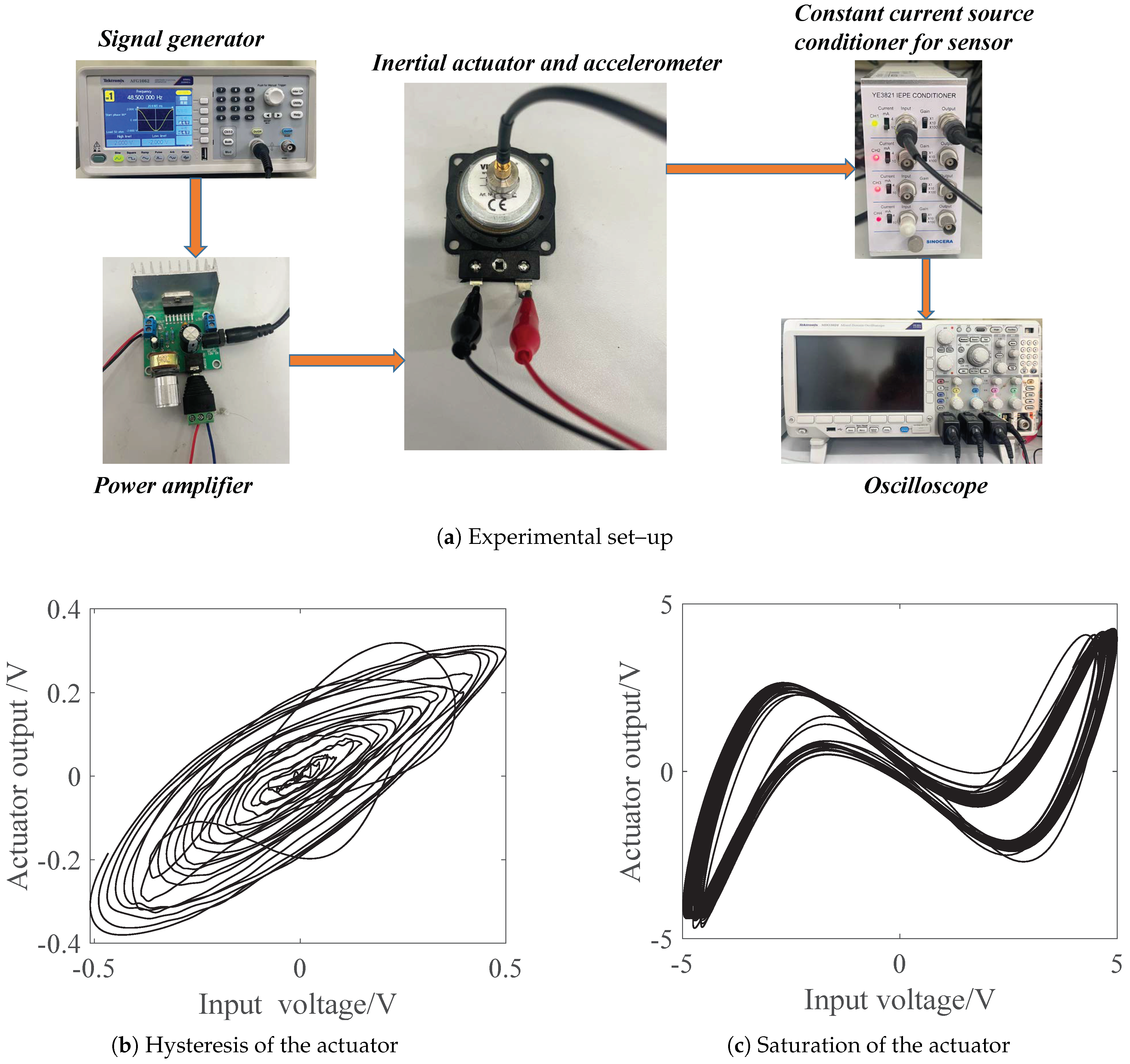
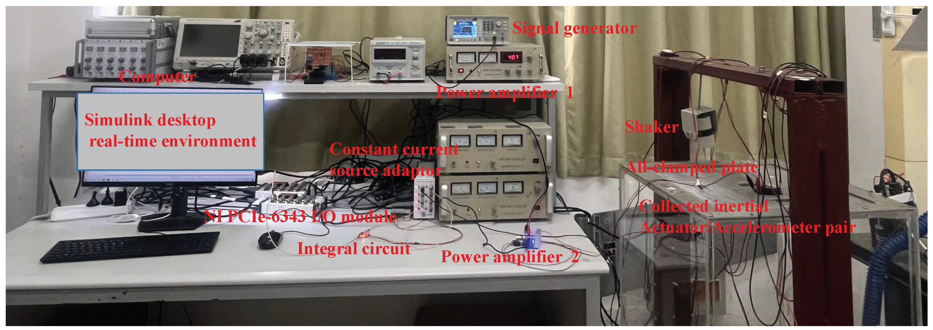
4.1. Experimental Set Up

4.1.1. Design of the Hardware Components

The experimental platform is shown in Figure 4, and the geometrical properties of the plate are summarized in

Table 1. Values of model parameters.

The dimensions of the plate $L_x\times L_y$	0.5 × 0.5 m
The thickness of the plate $L_z$	0.001 m
The mass density of the plate $\rho$	2700 kg/m${}^3$
The Young’s modulus of the plate E	7.1 × ${10}^{10}$ N/m
The Poisson ratio of the plate ${\nu }_s$	0.33
First resonant frequency f	48.6 Hz

. The signal transmission process is briefly described as follows. The excitation signal is given by the signal generator (Tektronix AFG1062) to simulate the external disturbances. An acceleration sensor is applied to collect the vibration signal, which passes through the constant current-source conditioner (YE3821) and the signal-conditioning circuit. In the Simulink desktop real-time simulation environment, the input value is calculated and output by the module port of PCIe to complete the vibration control.

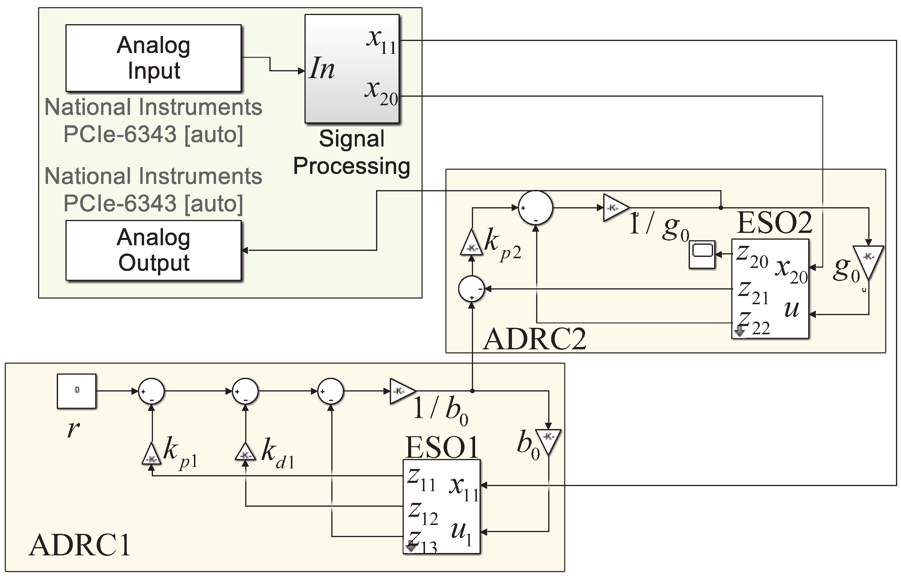
4.1.2. Software System Development

The software part is designed to create a real-time simulation. The main software required is MATLAB/Simulink R2018b, which requires a desktop real-time toolbox to be installed. The default compiler is Microsoft Visual C++ 2017. Some key configurations are as follows: The Analog Input and Analog Output modules configure the input and output of the NI PCIe-6343, which is set to 10 kHz here, that is, the sampling time is 0.0001 s. The operating mode is selected as external mode. The system target file selection is sldrt.tlc. Therefore, the controller of Section 3.2 can be built in Simulink as shown in Figure 5.

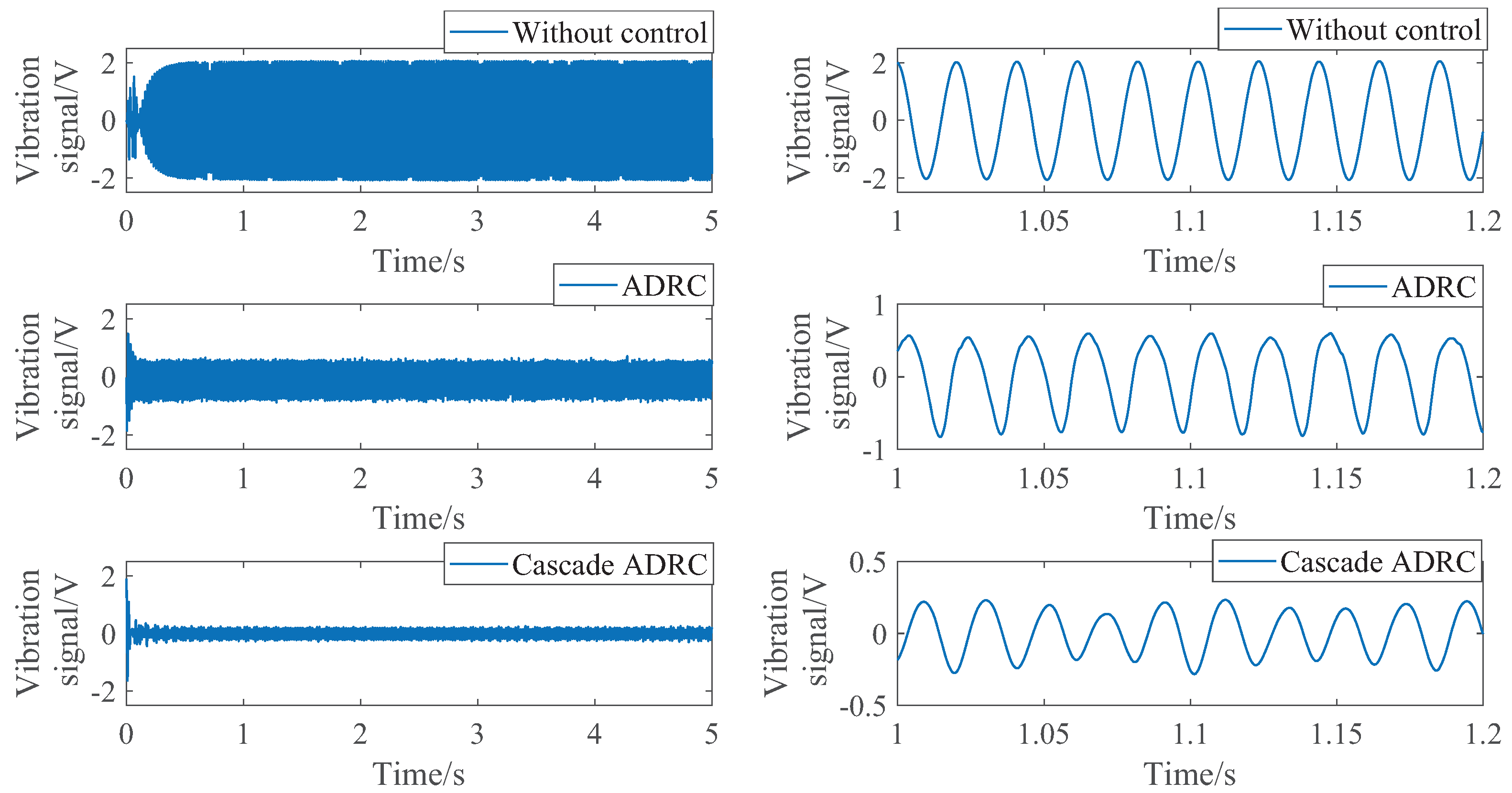
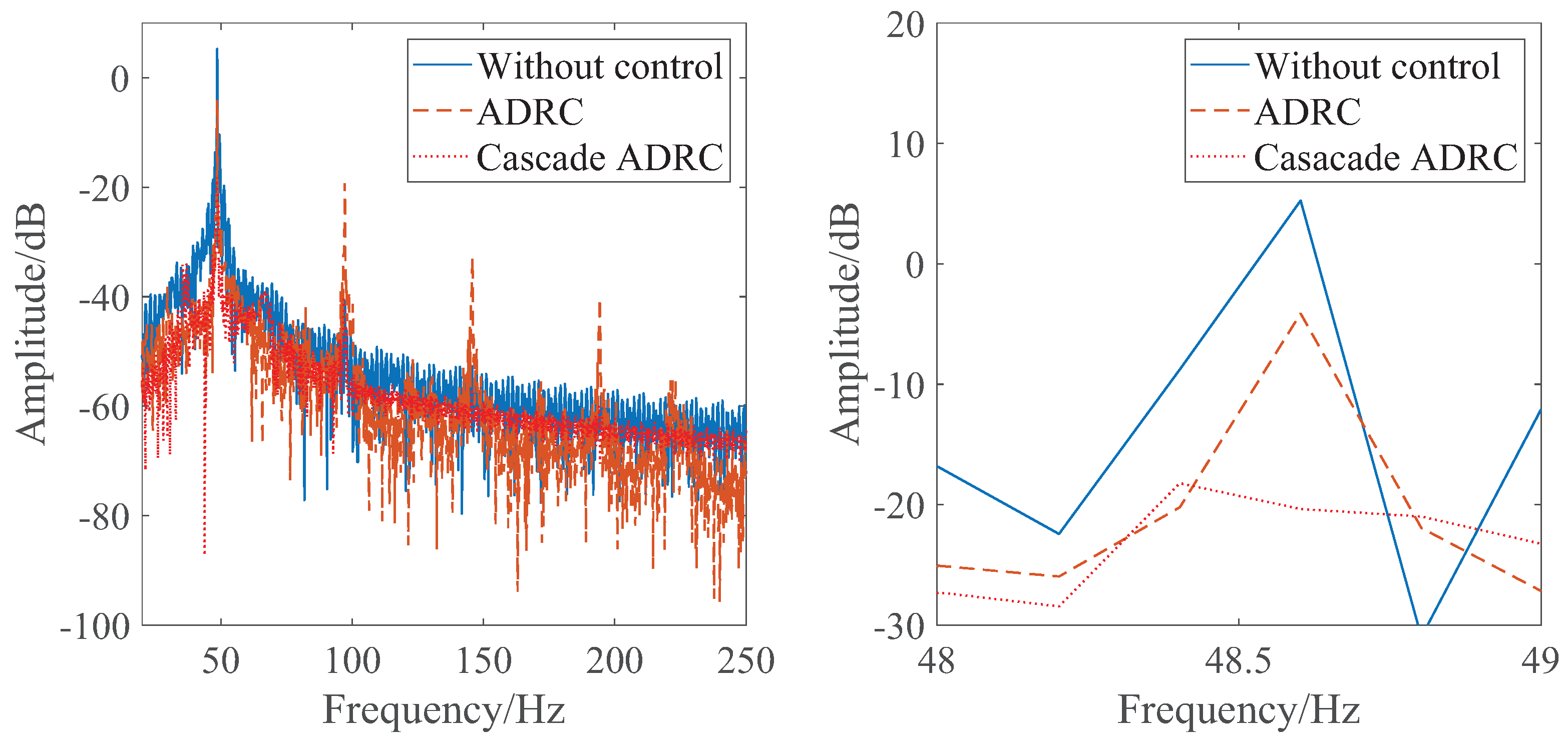
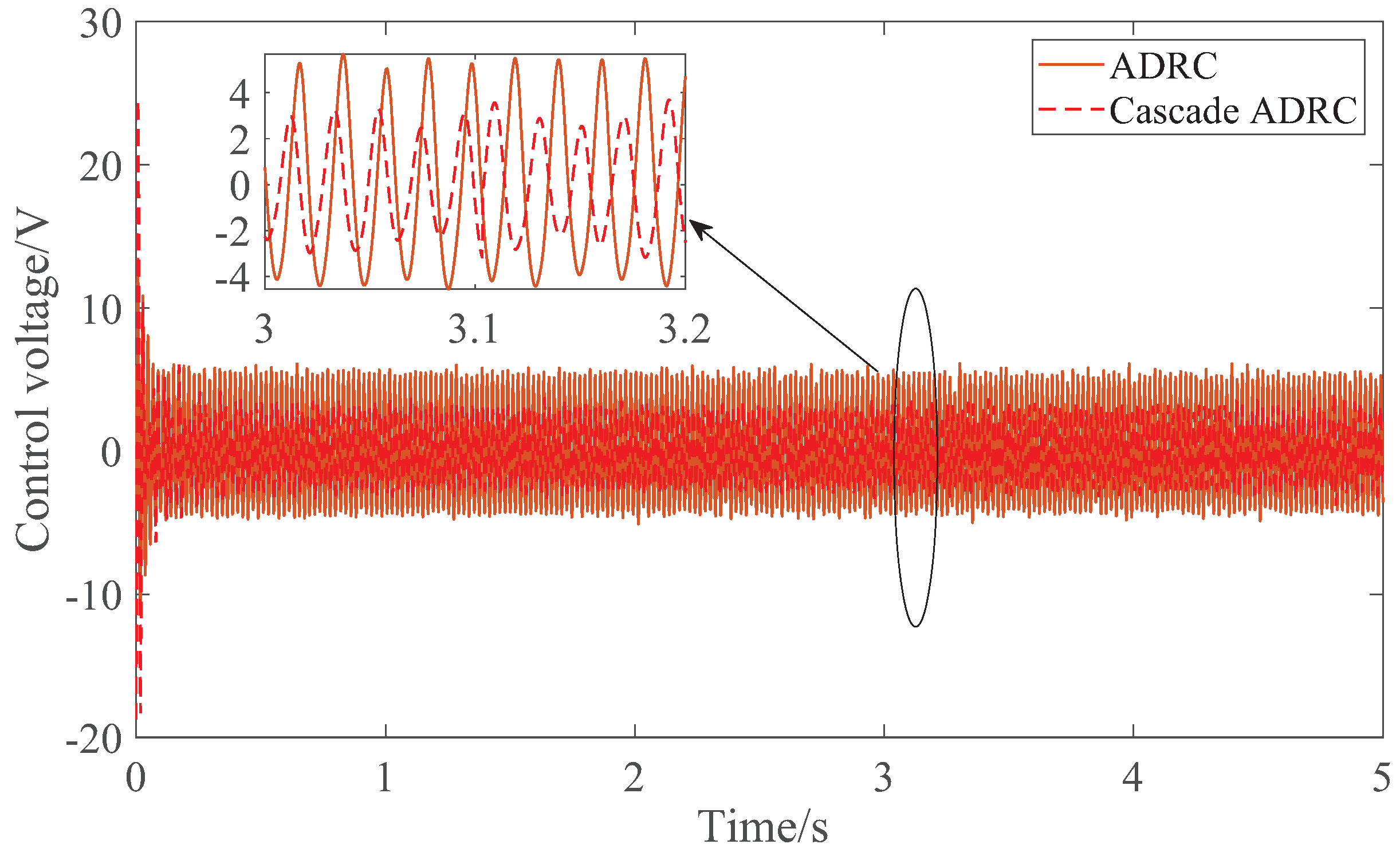
4.2. Experimental Results

The traditional second-order ADRC and cascade ADRC are adopted to control the vibration of the all-clamped plate experimental device. First, whether this particular system satisfies the stability conditions in Section 3.4 is checked. In the process of plate vibration, the changing rate of the structure state has a physical limit. For example, the sudden impact force is related to the change in the plate velocity with inertia. In brief, in the plate with the studied inertial actuator, the signals are differentiable with bounded derivatives, i.e., assumption 1 is satisfied. Therefore, under the condition of a reasonable selection of controller parameters, the stability of the system is guaranteed. When no controller is applied, as shown in Figure 6, the structure vibrates under an external excitation simulated by the shaker, with an amplitude of approximately 2 V in the time domain, and this external excitation continues to affect the structure. In the real-time control process, the second-order ADRC is applied. It can be found that the ADRC has a relatively good suppression effect on the structural vibration. Under the same excitation, the vibration amplitude of the structure is reduced by more than half, to 0.7 V. Then, carrying out the experiment of the cascade ADRC control, it can be found that the cascade ADRC has achieved a better vibration suppression performance. Under the cascade ADRC, the amplitude of the vibration is greatly reduced to around 0.3 V. It can be concluded that this is because, for a high-order system such as an all-clamped plate, the cascade control technology is used to decompose it into a cascade system composed of a second-order system, and then the design is combined with the idea of ADRC. Satisfactory vibration control can still be achieved without relying on the model in the presence of multiple disturbances.

Next, for fairness in comparison, similar to [10], the spectrum of the normalized signal is represented as follows:

$$\mathrm{The}\mathrm{decibel}\mathrm{vlaue}=20lo{g}_{10}\left(FFT(y/y_R)\right),$$

(16)

where $FFT(·)$ represents the Fourier Transformation, and the value of $y_R$ is set to 1 V as the standard value.

As shown in Figure 7, the results are more visible in the frequency domain. The excitation frequency, i.e., the effect comparison at the first-order resonance frequency, shows that when the conventional ADRC achieves a control effect of 9.37 dB, the effect of the cascade ADRC reaches 24.36 dB. In addition, at the double frequency worthy of attention, the cascade ADRC has also achieved better results, and the amplitudes of other frequency doubles are too small in comparison.

The control quantities of the ADRC and cascade ADRC are also compared, as shown in Figure 8. It is easily obtained that the control values based on the cascade ADRC are smaller than those under the traditional ADRC method. Therefore, a satisfactory experimental result is obtained to indicate that the vibration suppression performance under the cascade ADRC is better than that under the ADRC accompanied by less energy consumption.

In general, the cascade ADRC controller designed in this paper combines the classical active disturbance rejection controller and the cascade control technology to control the vibration of the all-clamped plate structure with an inertial actuator in real time, and it achieves a satisfactory control effect, which is fast and accurate, and the ability to suppress disturbance is strong.

5. Conclusions

Aiming at a multi-coupling, high-order, strong nonlinear all-clamped plate with an inertial actuator, a cascade ADRC controller is designed and a real-time control experiment of structural vibration suppression is carried out. The method proposed in this paper has a strong disturbance rejection performance and decoupling ability for nonlinear strongly coupled systems. Some conclusions are given as follows:

(1) The nonlinear dynamics of the system are demonstrated by experiments, which with only one sensor are simple, low-cost and convenient;

(2) The cascade ADRC based on inner and outer loops can achieve good control performance, and the anti-noise ADRC designed for the rapidity of inner loops can improve system performance;

(3) The parameter adjustment based on the bandwidth method is simple and has obvious physical meaning, which is suitable for engineering applications.

Compared with the traditional single-loop control, the disadvantages of the proposed cascade ADRC are mainly manifested in the following two aspects. First, the number of required sensors increases and thus the cost increases. In this paper, two accelerometers are used, which is one more sensor than the traditional single-loop control. Second, although some parameter tuning guides are given in this paper, the increase in the number of parameters will bring some troubles to parameter tuning. Future work will focus on how to improve on these shortcomings and make better use of the strengths of the cascade ADRC, such as inertial actuator self-sensing, improving the corresponding speed of the inner loop, etc.

References

1. Borgo, M.; Tehrani, M.; Elliott, S. Active nonlinear control of a stroke limited inertial actuator: Theory and experiment. J. Sound Vib. 2020, 465, 115009. [Google Scholar] [CrossRef]
2. Camperi, S.; Tehrani, M.; Elliott, S. Parametric study on the optimal tuning of an inertial actuator for vibration control of a plate: Theory and experiments. J. Sound Vib. 2018, 435, 1–22. [Google Scholar] [CrossRef] [Green Version]
3. Boulandet, R.; Michau, M.; Micheau, P.; Berry, A. Aircraft panel with sensorless active sound power reduction capabilities through virtual mechanical impedances. J. Sound Vib. 2016, 361, 2–19. [Google Scholar] [CrossRef]
4. Camperi, S.; Tehrani, M.; Elliott, S. Local tuning and power requirements of a multi-input multi-output decentralised velocity feedback with inertial actuators. Mech. Syst. Signal Process. 2019, 117, 689–708. [Google Scholar] [CrossRef] [Green Version]
5. Dáz, C.G.; Gardonio, P. Feedback control laws for proof-mass electrodynamic actuators. Smart Mater. Struct. 2007, 16, 1766–1783. [Google Scholar]
6. Airimitoaie, T.; Landau, I. Robust and Adaptive Active Vibration Control Using an Inertial Actuator. IEEE Trans. Ind. Electron. 2016, 63, 6482–6489. [Google Scholar] [CrossRef] [Green Version]
7. Cao, T.; Chen, L.; He, F.; Summut, K. Adaptive integral sliding mode control for active vibration absorber design. In Proceedings of the 39th IEEE Conference Decision and Control, Sydney, Australia, 12–15 December 2000; pp. 2436–2437. [Google Scholar]
8. Zhang, L.; Li, S.; Zhu, C.; Li, J. Eso-based vibration control for all-clamped plate using an electrodynamic inertial actuator. Int. J. Struct. Stab. Dyn. 2022, 22, 2250013. [Google Scholar] [CrossRef]
9. Borgo, M.; Tehrani, M.; Elliott, S. Identification and analysis of nonlinear dynamics of inertial actuators. Mech. Syst. Signal Process. 2019, 115, 338–360. [Google Scholar] [CrossRef] [Green Version]
10. Li, S.; Zhang, L.; Zhu, C.; Su, J.; Li, J. Nonlinear eso-based vibration control for an all-clamped piezoelectric plate with disturbances and time delay: Design and hardware implementation. J. Intell. Mater. Syst. Struct. 2022. [Google Scholar] [CrossRef]
11. Chi, R.; Li, H.; Shen, D.; Hou, Z.; Huang, B. Enhanced P-type Control: Indirect Adaptive Learning from Set-point Updates. IEEE Trans. Autom. Control 2022. [Google Scholar] [CrossRef]
12. Yu, S.; Ma, J.; Wu, H.; Kang, S. Robust precision motion control of piezoelectric actuators using fast nonsingular terminal sliding mode with time delay estimation. Meas. Control 2018, 52, 11–19. [Google Scholar] [CrossRef] [Green Version]
13. Chen, W.; Yang, J.; Guo, L.; Li, S. Disturbance-observer-based control and related methods—An overview. IEEE Trans. Ind. Electron. 2016, 63, 1083–1095. [Google Scholar] [CrossRef] [Green Version]
14. Wei, W.; Duan, B.; Zuo, M. Active disturbance rejection control for a piezoelectric nano-positioning system: A U-model approach. Meas. Control 2021, 54, 506–518. [Google Scholar] [CrossRef]
15. Han, J. From PID to Active Disturbance Rejection Control. IEEE Trans. Ind. Electron. 2009, 56, 900–906. [Google Scholar] [CrossRef]
16. Guo, B.; Bacha, S.; Alamir, M.; Hably, A.; Boudinet, C. Generalized Integrator-Extended State Observer with Applications to Grid-Connected Converters in the Presence of Disturbances. IEEE Trans. Control. Syst. Technol. 2021, 29, 744–755. [Google Scholar] [CrossRef]
17. Abdul-Adheem, W.; Ibraheem, I.; Humaidi, A.; Azar, A. Model-free active input-output feedback linearization of a single-link flexible joint manipulator: An improved active disturbance rejection control approach. Meas. Control 2021, 54, 856–871. [Google Scholar] [CrossRef]
18. Madonski, R.; Shao, S.; Zhang, H.; Gao, Z.; Yang, J.; Li, S. General error-based active disturbance rejection control for swift industrial implementations. Control Eng. Pract. 2019, 84, 218–229. [Google Scholar] [CrossRef]
19. Zhang, F.; Hou, J.; Ning, D.; Gong, Y. Depth Control of an Oil Bladder Type Deep-Sea AUV Based on Fuzzy Adaptive Linear Active Disturbance Rejection Control. Machines 2022, 10, 163. [Google Scholar] [CrossRef]
20. Roman, R.; Precup, R.; Petriu, E. Hybrid Data-Driven Fuzzy Active Disturbance Rejection Control for Tower Crane Systems. Eur. J. Control 2021, 58, 373–387. [Google Scholar] [CrossRef]
21. Zhang, H.; Li, Y.; Li, Z.; Zhao, C.; Gao, F.; Xu, F.; Wang, P. Extended-state-observer based model predictive control of a hybrid modular dc transformer. IEEE Trans. Ind. Electron. 2022, 69, 1561–1572. [Google Scholar] [CrossRef]
22. Baz, A. Active acoustic metamaterial with tunable effective density using a disturbance rejection controller. J. Appl. Phys. 2019, 125, 074503. [Google Scholar] [CrossRef]
23. Li, S.Q.; Zhu, C.W.; Mao, Q.B.; Su, J.Y.; Li, J. Active disturbance rejection vibration control for an all-clamped piezoelectric plate with delay. Control Eng. Pract. 2021, 108, 104719. [Google Scholar]
24. Hezzi, A.; Elghali, S.; Bensalem, Y.; Zhou, Z.; Benbouzid, M.; Abdelkrim, M. ADRC-Based Robust and Resilient Control of a 5-Phase PMSM Driven Electric Vehicle. Machines 2020, 8, 17. [Google Scholar] [CrossRef]
25. Díaz, I.; Pereira, E.; Hudson, M.; Reynolds, P. Enhancing active vibration control of pedestrian structures using inertial actuators with local feedback control. Eng. Struct. 2012, 41, 157–166. [Google Scholar] [CrossRef]
26. Huyanan, S.; Sims, N. Vibration control strategies for proof-mass actuators. J. Vib. Control 2007, 13, 1785–1806. [Google Scholar] [CrossRef] [Green Version]
27. Madonski, R.; Herman, P. Method of sensor noise attenuation in high-gain observers; Experimental verification on two laboratory systems. In Proceedings of the 2012 IEEE International Symposium on Robotic and Sensors Environments Proceedings, Magdeburg, Germany, 16–18 November 2012; pp. 121–126. [Google Scholar]
28. Xue, W.; Huang, Y. Performance analysis of 2-DOF tracking for a class of nonlinear uncertain systems with discontinuous disturbances. Int. J. Robust Nonlinear Control 2018, 28, 1456–1473. [Google Scholar] [CrossRef]
Figure 1. Characteristics of the inertial actuators.
Machines 10 00528 g001
Figure 2. Experimental research on system nonlinearity.
Machines 10 00528 g002
Figure 3. Schematic representation of the cascade ADRC control structure.
Machines 10 00528 g003
Figure 4. Photo of the hardware-in-the-loop experiment platform.
Machines 10 00528 g004
Figure 5. Real-time simulation model of cascade ADRC in Simulink.
Machines 10 00528 g005
Figure 6. Control performance in time domain: globe–response curves and local–response curves.
Machines 10 00528 g006
Figure 7. Control performance in frequency domain: globe–response curves and local–response curves.
Machines 10 00528 g007
Figure 8. Experimental control–voltage curves.
Machines 10 00528 g008