Comprehensive and Simplified Fault Diagnosis for Three-Phase Induction Motor Using Parity Equation Approach in Stator Current Reference Frame

Abstract

In this paper, a complementary and simplified scheme to diagnose electrical faults in a three-phase induction motor using the parity equations approach during steady state operation bases on the stator current reference frame is presented. The proposed scheme allows us to identify the motor phase affected due to faults related to the stator side, such as current sensors, voltage sensors, and resistance. The results obtained in this work complement a detection system that uses the DQ model of the three-phase induction motor and parity equations focused on the synchronous reference frame, which can detect stator-side faults but cannot locate the affected phase. In addition, considering practical and operational aspects, the residual detection set obtained is simplified to three simple algebraic equations that are easy to implement. The simulation results using the PSIM simulation software and the experimental test allow us to validate the proposed scheme.

1. Introduction

Currently, the induction motor (IM) is the horsepower in a wide variety of industrial processes and is often found embedded in many critical applications. The reliability and lifetime of the equipment can be increased by executing maintenance programs prior to a suitable fault diagnosis in the IM. Commonly, the most frequent faults in IM are related to a stress operation such as local overheating, unbalance supply voltages and interturn short-circuit in the stator winding [1]. These stress operations cause changes in the IM electrical-mechanic parameters and can be quickly diagnosed by determining the fault location, as well as its detection time delay. Regarding mechanical failures, vibration analysis using accelerometers is the most used technique due to the large magnitudes of the signals and the high immunity to electromagnetic interference. the only problem is the low bandwidth. Other authors have worked with intelligent systems using neural networks to detect bearing faults but offline and without considering input disturbances [2], although in [3] an adaptive neural network was used to correct these two disadvantages. However, the main problems of these types of techniques are long response time, computational complexity and high data storage. On the other hand, In the literature, there are many techniques to detect failure by mechanical and electrical faults in the IM. For example, by phase spectral analysis of current [4], by phase current transformation [5], by voltage unbalance at the neutral terminal [6] and by impedances unbalance [7]. The problem found in the previous techniques is that the location and detection time are very long, although for incipient failures the early detection time are not strictly necessary. Model-based methods with different approaches often have short response times to detect faults, such as the winding function approach to detect stator winding faults in the IM [1], or the parity equations approach to detect a large set of faults in the CD motor [8]. The problem is that an accurate mathematical model must be obtained. Regarding the parity equations approach, the model uncertainties and the high sensitivity to noise are the main problems, so this type of approach has been commonly used in linear or linearized systems [8]. However, there are works that focus on nonlinear systems but commonly use discrete time polynomial models [9], then the computational complexity and recursive values increase. Commonly, the fault diagnosis procedure is based on heuristic knowledge of the process as well as a priori knowledge of fault symptom causalities and stored data [10]. However, the approach based on parity equations using analytical symptoms with fixed or adaptive thresholds to detect changes in the residuals and without a stored data bank allows for minimal mathematical complexity, which simplifies and facilitates the implementation of detection residues [11]. Additionally, in the literature, other authors discretize the nonlinear model of the IM to diagnose only sensor faults, losing sight of the faults in the system parameters [2]. On the other hand, some authors propose a parity equation scheme applied to a nonlinear three-phase induction motor using the DQ synchronous reference frame matching the IM model with the DC motor model. This last strategy achieves a simple residual set of information that allows a wide detection of electrical and mechanical parameters during the steady state operation, but the fault isolation concerning each phase is not obtained [12,13]. On the other hand, in [14] a very simple method to insulate only the stator current sensor fault using the average normalized currents applied for PMSM drives is proposed. The idea is very good, but it does not help us to identify the damage parameters related to the stator side, such as current sensors, voltage sensors, and resistance.

In this work, a new complementary scheme to improve the diagnosis system proposed in [12] and [13] is proposed. In this way, to detect and isolate electrical faults in the stator side by phase, a new linear model based on the stator reference frame during steady state operation and a classical fault detection approach based on parity equations are proposed. Then a residual set of simplified equations are obtained, which could be easily implemented using modest digital processors.

This manuscript is structured as follows. Section 2 highlights the importance of this work and presents the methodology to follow. Additionally, the fault detection method using parity equations and the case study applied to IM using the DQ reference frame are presented. Section 3 presents the three-phase IM model developed based on the stator reference frame. Section 4 is dedicated to fault detection in the IM with parity equations using the model obtained in the previous section. Section 5 presents the residual set obtained and these are validated through experimental and simulation tests.

2. Motivation

As mentioned in the previous section, the literature presents many approaches to diagnose failures. In general, reference [11] presents many signal-based and model-based fault detection methods, highlighting their advantages and disadvantages. Regarding the fault diagnosis in rotating machinery [4], the consensus is that the high computational complexity and high data storage capacity are the common factors between them, even more so if the fault diagnosis considers the dynamic state of IM with variable speed. However, there are many critical applications at constant speed that are the bottleneck in many production processes, such as conveyor belts, ventilation, drilling, etc., where online diagnosis can be very useful. In this way, a simple online fault diagnosis system for each IM is very useful to schedule corrective maintenance focused on the parameter that is particularly affected. This work focuses particularly on complementing the electrical fault diagnosis proposed in [12,13], which uses parity equations in the DQ synchronous reference frame where the main problem is to identify the affected phase. In this way, the main idea of this work is to generate a residual set based on the stator current reference frame to distinguish the damaged phases.

In this section, the well-known theory of parity equations is shown and subsequently its application to diagnose faults in the IM using the DQ reference frame proposed in [13] and the problem encountered is highlighted. Figure 1 shows the general scheme for model-based fault detection [11]; on the right, the methodology carried out in this work to obtain faults applied to the IM working in stable state at constant speed is shown.

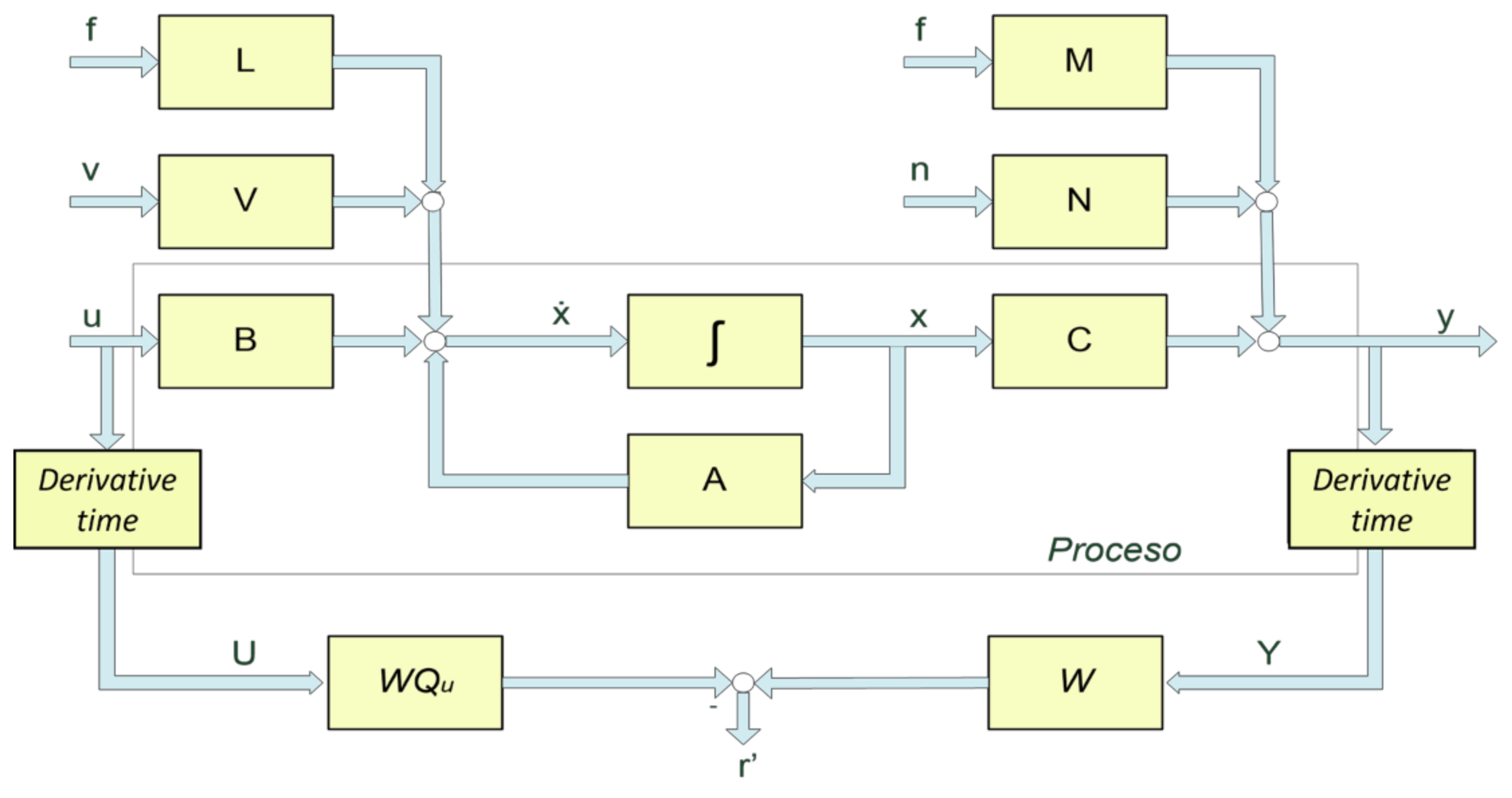
2.1. Parity Equations for Fault Diagnostic

The inconsistency between current and expected failures is expressed mathematically in residuals. Quantitatively, the residuals are zero if there is no disturbance or failure in the system. The residual generation is the main issue in model-based fault diagnosis. A variety of methods are available in literature for fault diagnosis. Most of these techniques are based on both continuous and discrete system models; however, in this issue, the attention is focused only on parity equation.

A block diagram of a fault diagnosis scheme based on the parity equation using state spaces, widely studied in [15,16], is shown in Figure 2.

From Figure 1, v(t) and n(t) are input/output noise disturbances, respectively, f(t) is the additive fault that can be composed of additive input faults f_l(t) and additive output faults f_m(t). Then

$${\mathrm{f}}^{\mathrm{T}}\left(t\right)=\left[{\mathrm{f}}_{\mathrm{m}}^{\mathrm{T}}\left(t\right){ \mathrm{f}}_{\mathrm{l}}^{\mathrm{T}}\left(t\right)\right]$$

(1)

where the first derivate is:

$$\begin{gathered} \dot{\mathrm{y}}\left(t\right)=\mathrm{C}\dot{\mathrm{x}}\left(t\right)+\mathrm{N}\dot{\mathrm{n}}\left(t\right)+\mathrm{M}\dot{\mathrm{f}}\left(t\right) \\ =\mathrm{C} \mathrm{A} \mathrm{x}\left(t\right)+\mathrm{C} \mathrm{B} \mathrm{u}\left(t\right)+\mathrm{C} \mathrm{V} \mathrm{v}\left(t\right)+\mathrm{C} \mathrm{L} \mathrm{f}\left(t\right)+\mathrm{N}\dot{\mathrm{n}}\left(t\right)+\mathrm{M}\dot{\mathrm{f}}\left(t\right) \end{gathered}$$

(2)

The second derivative is as follows:

$$\begin{gathered} \ddot{\mathrm{y}}\left(t\right)=\mathrm{C} \ddot{x}\left(t\right)+\mathrm{N} \ddot{\mathrm{n}}\left(t\right)+\mathrm{M} \ddot{\mathrm{f}}\left(t\right) \\ ={\mathrm{CA}}^2\mathrm{x}\left(t\right)+\mathrm{C} \mathrm{A} \mathrm{B} \mathrm{u}\left(t\right)+\mathrm{C} \mathrm{B} \dot{\mathrm{u}}\left(t\right)+\mathrm{C} \mathrm{A} \mathrm{V} \mathrm{v}\left(t\right)+\mathrm{C} \mathrm{V}\dot{\mathrm{v}}\left(t\right)+\mathrm{N} \ddot{\mathrm{n}}\left(t\right)+ \mathrm{C} \mathrm{A} \mathrm{L} \mathrm{f}\left(t\right) \\ +\mathrm{C} \mathrm{L}\dot{\mathrm{f}}\left(t\right)+\mathrm{M}\ddot{\mathrm{f}}\left(t\right) \end{gathered}$$

(3)

In this way, redundancy is generated in the equation, at the same time t increases its derivatives q ≤ n of Y(t), which leads to a system of equations as follows:

$$\mathrm{Y}\left(t\right)=\mathrm{T} \mathrm{x}\left(t\right)+{ \mathrm{Q}}_{\mathrm{u}} \mathrm{U}\left(t\right)+{\mathrm{Q}}_{\mathrm{v}} \mathrm{V}\left(t\right)+{\mathrm{Q}}_{\mathrm{n}} \mathrm{N}\left(t\right)+{\mathrm{Q}}_{\mathrm{f}} \mathrm{F}\left(t\right)$$

(4)

where:

$$\begin{gathered} \mathrm{Y}\left(t\right)=\left[\begin{array}{c}\mathrm{y}\left(\mathrm{t}\right)\\ \dot{\mathrm{y}}\left(\mathrm{t}\right)\\ \begin{array}{c}⋮\\ {\mathrm{y}}^{\left(\mathrm{q}\right)}\left(\mathrm{t}\right)\end{array}\end{array}\right] \mathrm{U}\left(t\right)=\left[\begin{array}{c}\mathrm{u}\left(t\right)\\ \dot{\mathrm{u}}\left(t\right)\\ \begin{array}{c}⋮\\ {\mathrm{u}}^{\left(\mathrm{q}\right)}\left(t\right)\end{array}\end{array}\right] \mathrm{V}\left(t\right)=\left[\begin{array}{c}\mathrm{v}\left(t\right)\\ \dot{\mathrm{v}}\left(t\right)\\ \begin{array}{c}⋮\\ {\mathrm{v}}^{\left(\mathrm{q}\right)}\left(t\right)\end{array}\end{array}\right] \mathrm{F}\left(t\right)=\left[\begin{array}{c}\mathrm{f}\left(t\right)\\ \dot{\mathrm{f}}\left(t\right)\\ \begin{array}{c}⋮\\ {\mathrm{f}}^{\left(\mathrm{q}\right)}\left(t\right)\end{array}\end{array}\right] \\ \mathrm{T} =\left[\begin{array}{c}\mathrm{C} \\ \mathrm{C}\mathrm{A}\\ {\mathrm{CA}}^2\\ \begin{array}{c}⋮\\ {\mathrm{CA}}^{\mathrm{q}}\end{array}\end{array}\right] \end{gathered}$$

(5)

$${\mathrm{Q}}_{\mathrm{U}}=\left[\begin{array}{ccc}\begin{array}{ccc}\begin{array}{c}0\\ \mathrm{C} \mathrm{B}\\ \mathrm{C} \mathrm{A} \mathrm{B} \end{array}& \begin{array}{c}0\\ 0\\ \mathrm{C} \mathrm{B}\end{array}& \begin{array}{c}0\\ 0\\ 0\end{array}\end{array}& \begin{array}{c}\cdots \\ \dots \\ \cdots \end{array}& \begin{array}{c}0\\ 0\\ 0\end{array}\\ \begin{array}{cc}⋮& ⋮\end{array}& \ddots & ⋮\\ \begin{array}{ccc}{\mathrm{C} \mathrm{A}}^{\mathrm{q}-1}\mathrm{B}& {\mathrm{C} \mathrm{A}}^{\mathrm{q}-2}\mathrm{B}& \dots \end{array}& \mathrm{C} \mathrm{B}& 0\end{array}\right]$$

(6)

$${\mathrm{Q}}_{\mathrm{v}}=\left[\begin{array}{ccc}\begin{array}{ccc}\begin{array}{c}\mathrm{N}\\ \mathrm{C} \mathrm{V}\\ \mathrm{C} \mathrm{A} \mathrm{V} \end{array}& \begin{array}{c}0\\ \mathrm{N}\\ \mathrm{C} \mathrm{V}\end{array}& \begin{array}{c}0\\ 0\\ \mathrm{N}\end{array}\end{array}& \begin{array}{c}\cdots \\ \dots \\ \cdots \end{array}& \begin{array}{c}0\\ 0\\ 0\end{array}\\ \begin{array}{cc}⋮& ⋮\end{array}& \ddots & ⋮\\ \begin{array}{ccc}{\mathrm{C} \mathrm{A}}^{\mathrm{q}-1}\mathrm{V}& {\mathrm{C} \mathrm{A}}^{\mathrm{q}-2}\mathrm{V}& \dots \end{array}& \mathrm{C} \mathrm{V}& \mathrm{N}\end{array}\right]$$

(7)

$${\mathrm{Q}}_{\mathrm{f}}=\left[\begin{array}{ccc}\begin{array}{ccc}\begin{array}{c}\mathrm{M}\\ \mathrm{C} \mathrm{L}\\ \mathrm{C} \mathrm{A} \mathrm{L} \end{array}& \begin{array}{c}0\\ \mathrm{M}\\ \mathrm{C} \mathrm{L}\end{array}& \begin{array}{c}0\\ 0\\ \mathrm{M}\end{array}\end{array}& \begin{array}{c}\cdots \\ \dots \\ \cdots \end{array}& \begin{array}{c}0\\ 0\\ 0\end{array}\\ \begin{array}{cc}⋮& ⋮\end{array}& \ddots & ⋮\\ \begin{array}{ccc}{\mathrm{C} \mathrm{A}}^{\mathrm{q}-1}\mathrm{L}& {\mathrm{C} \mathrm{A}}^{\mathrm{q}-2}\mathrm{L}& \dots \end{array}& \mathrm{C} \mathrm{L}& 0\end{array}\right]$$

(8)

For a system of order n with p inputs, where p_v is the number of disturbances and r the outputs of the matrices with the following dimensions:

• $\mathrm{Y}\left(t\right)$ is a vector $\left(q+1\right)r \mathrm{x} 1$
• $\mathrm{U}\left(t\right)$ is a vector $\left(q+1\right)p \mathrm{x} 1$
• $\mathrm{T}$ is a matrix $\left(q+1\right)r \mathrm{x} n$
• ${\mathrm{Q}}_{\mathrm{U}}$ is a matrix $\left(q+1\right)r \mathrm{x} \left(q+1\right)p$
• ${\mathrm{Q}}_{\mathrm{v}}$ is a matrix $\left(q+1\right)r \mathrm{x} \left(q+1\right)p_v$

Since the vector of states x(t) and the disturbance $v\left(t\right)$ are unknown in (4) is multiplied by a vector $w^T$:

$${\mathrm{w}}^{\mathrm{T}}{\mathrm{Y}}^{\mathrm{T}}={\mathrm{w}}^{\mathrm{T}} \mathrm{T} \mathrm{x}\left(t\right)+{\mathrm{w}}^{\mathrm{T}}{ \mathrm{Q}}_{\mathrm{u}} \mathrm{U}\left(t\right)+{\mathrm{w}}^{\mathrm{T}}{ \mathrm{Q}}_{\mathrm{v}} \mathrm{V}\left(t\right)+{\mathrm{w}}^{\mathrm{T}}{ \mathrm{Q}}_{\mathrm{n}} \mathrm{N}\left(t\right)+{\mathrm{w}}^{\mathrm{T}}{ \mathrm{Q}}_{\mathrm{f}} \mathrm{F}\left(t\right)$$

(9)

Then W^T must have a dimension $\left(1 x \left(q+1\right)·r\right)$ such that:

$${\mathrm{w}}^{\mathrm{T}} \mathrm{T}=0 y {\mathrm{w}}^{\mathrm{T}}{ \mathrm{Q}}_{\mathrm{v}}=0$$

(10)

Now, a residual vector in computational form is obtained as follows:

$$\mathrm{r}\left(t\right)={\mathrm{w}}^{\mathrm{T}} \mathrm{Y}\left(t\right)-{\mathrm{w}}^{\mathrm{T}}{ \mathrm{Q}}_{\mathrm{u}} \mathrm{U}\left(t\right)$$

(11)

Through Equation (10), a part of the elements of $w^T$ is determined according to the order of $T$ and $Q_v$. The remaining elements can be used to design different parity equations. Inserting (9) into (11), the internal form of the parity equation is given as follows:

$$\mathrm{r}\left(t\right)={\mathrm{w}}^{\mathrm{T}}{ \mathrm{Q}}_{\mathrm{f}} \mathrm{F}\left(t\right)+{\mathrm{w}}^{\mathrm{T}}{ \mathrm{Q}}_{\mathrm{n}} \mathrm{N}\left(t\right)$$

(12)

which shows how the residual is affected by the faults in $F\left(t\right)$ and the noise $N\left(t\right)$. If (10) is satisfied, the remainder is independent of the unknown input $\mathrm{v}\left(\mathrm{t}\right)$ and the state $x\left(t\right)$. More residues are obtained by selecting several different vectors $w^T$, thus forming a matrix $W$ and the residual vector finally becomes

$$\mathrm{r}\left(t\right)=\mathrm{W} \mathrm{Y}\left(t\right)-{\mathrm{WQ}}_{\mathrm{u}}\mathrm{U}\left(t\right)$$

(13)

Then, the order of $W$ determines the number of residues in the system to analyze.

2.2. Fault Diagnosis Using DQ Reference Frame for Induction Motor

The starting point to carry out the analysis of the IM model in the synchronous reference frame is to deduce the transfer functions in the subsystems of the mechanical and electrical sections. The main idea is to match analytically the three-phase induction motor model with the DC motor model, making use of the DQ transformation. Additionally, the definition of the parameters of the DQ model with respect to the parameters of the IM model are found, to define the equation of state spaces for fault diagnostic.

For mechanical and electrical parts to be coupled, there is a link between the current produced by the torque and the induced magnetic force. This link is implicit in the total current loop of the motor and is independent of the mechanical part in the transfer function [17]. This model is similar to the DC motor model obtained in [18]; the main differences are that the input parameter is instead of the armature current and the DC motor model parameters are analytically reassigned as follows.

$$\begin{gathered} L_a=\left(L_s-\frac{L_m{}^2}{L_r}\right) \\ {R}_a=R_s+\frac{L_s}{L_r}{R}_r \\ {K}_f=\left(\frac{3P}{4}\frac{L_m{}^2}{L_r}\right)i_f \\ \psi =L_s, i_f=L_s I_{ds} \end{gathered}$$

The system and fault diagnosis model based on the DQ synchronous reference frame results in an extensive residual set with derivative values. However, a significant reduction can be easily obtained if we consider only the behavior in the steady state. Therefore, the derivatives terms involving current, voltage and speed, $I_{qs}$, $V_{qs}$, ${\omega }_r$ respectively, are neglected, so the residual set is:

$$\begin{array}{c}{r}_1\left(t\right)=R_a·I_{qs}+\psi ·{\omega }_r-V_{qs}\\ r_2\left(t\right)=-(K_f·N_p)·I_{qs}+\left(B+B_l\right)·{\omega }_r\\ r_3\left(t\right)=\left[\psi ·K_f·N_p+R_a·\left(B+B_l\right)\right]·I_{qs}-\left(B+B_l\right)·V_{qs}\\ r_4\left(t\right)=\left[\psi ·K_f·N_p+R_a·\left(B+B_l\right)\right]·{\omega }_r-K_f·N_p·V_{qs}\end{array}$$

(14)

Finally, in the residual set obtained, it can be observed that the system of equations can be easily implemented using a modest digital processing system, because the equations are very simple algebraic expressions without any matrix or derivative terms.

Table 1. Fault detection matrix using the DQ Model.

Faults		${\mathbf{r}}_1$	${\mathit{r}}_2$	${\mathbf{r}}_3$	${\mathbf{r}}_4$
Parametric	${\mathrm{R}}_{\mathrm{s}}$	I	0	0	I
	${\mathrm{R}}_{\mathrm{r}}$	I	0	0	I
	${\mathrm{L}}_{\mathrm{s}}$	I	0	I	I
	${\mathrm{L}}_{\mathrm{r}}$	I	I	I	I
	$\mathrm{B}$	0	I	I	I
	${\mathrm{B}}_{\mathrm{l}}$	0	I	I	I
Additive	${\mathrm{i}}_{\mathrm{qs}}$	I	I	I	0
	${\mathsf{\omega }}_{\mathrm{r}}$	I	I	0	I
	${\mathrm{V}}_{qs}$	I	0	I	I

“I” represents a change positive or negative.

shows the residuals set, and many detectable parameters can be observed due to the different signatures that the residuals have at the failure of each parameter. Therefore, these parameters can be detected 100%. However, there are parameters that have the same signature, so the probability of failure is reduced to 50%, as seen in Table 1. For example, the signature (Rs, Rr), (B, Bl), (Ls, Vqs). Additionally, the final detection matrix cannot distinguish the damaged phase from the three-phase system, which represents the main problem in this work.

This fault diagnosis scheme based on the DQ reference frame was implemented for educational purposes in the LabVIEW development platform [19]. However, the simplicity of the equations and the open-loop diagnosis make its implementation feasible in an industrial system using more inexpensive development tools.

3. Three-Phase Induction Motor Model Based on Stator Current Reference Frame

In this section, we propose the use of the steady state dynamic equations of the motor, focusing on the stator current without mechanical parameters. The objective of this analysis is to involve the phases of three-phase system in order to identify faults and complement the diagnosis of the previous section.

First, the well-known equations that define the stator and rotor voltages, $V_s$ and $V_r$, respectively, of the induction motor for any of its three phases are [20]:

$$V_{si}=R_s{I}_{si}+\frac{d{\lambda }_{si}}{dt}$$

(15)

$$V_{ri}=R_r{I}_{ri}+\frac{d{\lambda }_{ri}}{dt}$$

(16)

where the subscript i represents the phase of induction motor (a, b, c). The magnetic flux is given by:

$${\lambda }_{si}=L_s{I}_{si}+M{I}_{ri}$$

(17)

$${\lambda }_{ri}=L_r{I}_{si}+M^T{I}_{si}$$

(18)

where

$$\begin{gathered} M=m_{sr}\left[\begin{array}{ccc}\cos \theta & \cos \left(\theta +\frac{2\pi }{3}\right)& \cos \left(\theta -\frac{2\pi }{3}\right)\\ \cos \left(\theta -\frac{2\pi }{3}\right)& \cos \theta & \cos \left(\theta +\frac{2\pi }{3}\right)\\ \cos \left(\theta +\frac{2\pi }{3}\right)& \cos \left(\theta -\frac{2\pi }{3}\right)& \cos \theta \end{array}\right] \\ {L}_s=\left[\begin{array}{ccc}{L}_{sa}& 0& 0\\ 0& L_{sb}& 0\\ 0& 0& L_{sc }\end{array}\right] L_r=\left[\begin{array}{ccc}{L}_{ra}& 0& 0\\ 0& L_{rb}& 0\\ 0& 0& L_{rc}\end{array}\right] \end{gathered}$$

(19)

Now, a matrix representation of the electrical behavior of the motor is obtained by replacing the magnetic flux

$$\left[\begin{array}{c}{V}_{si}\\ V_{ri}\end{array}\right]=\left[\begin{array}{cc}{R}_s& 0\\ 0& R_r\end{array}\right]\left[\begin{array}{c}{I}_{si}\\ I_{ri}\end{array}\right]+\frac{d}{dt}\left(\left[\begin{array}{cc}{L}_s& M\\ M^T& L_r\end{array}\right]\left[\begin{array}{c}{I}_{si}\\ I_{ri}\end{array}\right]\right)$$

(20)

A more straightforward and analogous way to represent the above would be:

$$V=R I+\frac{d}{dt}\left(L I\right)$$

(21)

where L can be expressed as the addition of $L1$ and $M1$ to separate the parameters $L_s$ and $L_r$ from the matrix M. Furthermore, L can be expressed as:

$$L=\left[\begin{array}{cc}{L}_s& M\\ M^T& L_r\end{array}\right]=\left[\begin{array}{cc}{L}_s& 0\\ 0& L_r\end{array}\right]+\left[\begin{array}{cc}0& M\\ M^T& 0\end{array}\right]$$

(22)

where

$$\begin{gathered} \left[\begin{array}{cc}{L}_s& 0\\ 0& L_r\end{array}\right]=L_1 \\ \left[\begin{array}{cc}0& M\\ M^T& 0\end{array}\right]=M_1 \end{gathered}$$

Then (21) is modified as follows

$$V=R I+\frac{d}{dt}\left(L_{1}I\right)+\frac{d}{dt}\left(M_1 I\right)$$

(23)

Because M₁ I contains time-varying elements, this derivation implies the use of the string rule, therefore.

$$\frac{d}{dt}\left(M_1 I\right)=\frac{d{M}_1}{dt}I+M_1\frac{dI}{dt}$$

(24)

Now, (23) is redefined as:

$$\frac{d{M}_1}{dt}I+M_1\frac{dI}{dt}+L_1\frac{dI}{dt}+R I=V$$

(25)

Then, the vector representation for the stator and rotor voltages in the motor, respectively, are:

$$V_{si}=R_s{I}_{si}+L_s{\dot{I}}_{si}+\dot{M}{I}_{ri}+M{\dot{I}}_{ri}$$

(26)

$$V_{ri}=R_r{I}_{ri}+L_r{\dot{I}}_{ri}+\dot{M^T}{I}_{si}+M^T{\dot{I}}_{si}$$

(27)

In this work, the steady state operation condition is considered, then $I_{ri}=0$ and $V_{ri}=0$, so the above equation is reduced as follows:

$$V_{si}=R_s{I}_{si}+L_s\dot{I_{si}}$$

(28)

$$0=\dot{M^T}{I}_{si}+M^T\dot{I_{si}}$$

(29)

The above expressions can be rewritten considering only the subsequent derivatives of the stator current. Then, the state space system is simplified, where $I_s$ and $V_s$ are the state and input variables, respectively, as follows.

$${\dot{I}}_s=-L_s{}^{-1}{R}_s{I}_s+L_s{}^{-1}{V}_s$$

(30)

Now, the state space equation based on stator current reference frame is considered without disturbances and without external faults. Where the output y(t) is a function of $I_{si}$ with a unitary matrix C.

$$y\left(t\right)=\left[\begin{array}{ccc}1& 0& 0\\ 0& 1& 0\\ 0& 0& 1\end{array}\right]\left[\begin{array}{c}{I}_{sa}\\ I_{sb}\\ I_{sc}\end{array}\right],\hspace{1em}\hspace{1em}\hspace{0.17em}u\left(t\right)=\left[\begin{array}{c}{V}_{sa}\\ V_{sb}\\ V_{sc}\end{array}\right]$$

Also, according to the three-phase IM model

$$\dot{x}=\dot{I_s}=\left[\begin{array}{c}\dot{{\mathrm{I}}_{sa}}\\ \dot{{\mathrm{I}}_{sb}}\\ \dot{{\mathrm{I}}_{sc}}\end{array}\right], x=I_s=\left[\begin{array}{c}{I}_{sa}\\ I_{sb}\\ I_{sc}\end{array}\right], \mathit{A}=-{\left[L_S\right]}^{-1}\left[R_S\right], \mathit{B}={\left[L_S\right]}^{-1}$$

where $L_s$, $R_s$ and $m_{sr}$ are defined as follows, according to [20]

$$Ls=\left[\begin{array}{ccc}{L}_{sa}+m_{sr}& -0.5 m_{sr}& -0.5 m_{sr}\\ -0.5 m_{sr}& L_{sb}+m_{sr}& -0.5 m_{sr}\\ -0.5 m_{sr}& -0.5 m_{sr}& L_{sc}+m_{sr}\end{array}\right], Rs=\left[\begin{array}{ccc}{R}_{sa}& 0& 0\\ 0& R_{sb}& 0\\ 0& 0& R_{sc}\end{array}\right], m_{sr}=\frac{2}{3}{l}_m$$

Now, solving and simplifying $A=-{\left[L_S\right]}^{-1}\left[R_S\right]$ and $B={\left[L_S\right]}^{-1}$ it is obtained that

$$A=\left[\begin{array}{ccc}{a}_{11}& a_{12}& a_{13}\\ a_{21}& a_{22}& a_{23}\\ a_{31}& a_{32}& a_{33}\end{array}\right]=\left[\begin{array}{ccc}-\frac{A1 R_{sa}}{k1}& -\frac{A2 R_{sb}}{k1}& -\frac{A3 R_{sc}}{k1}\\ -\frac{A2 R_{sa}}{k1}& -\frac{A5 R_{sb}}{k1}& -\frac{A6 R_{sc}}{k1}\\ -\frac{A3 R_{sa}}{k1}& -\frac{A6 R_{sb}}{k1}& -\frac{A9 R_{sc}}{k1}\end{array}\right]$$

(31)

$$B=\left[\begin{array}{ccc}{b}_{11}& b_{12}& b_{13}\\ b_{21}& b_{22}& b_{23}\\ b_{31}& b_{32}& b_{33}\end{array}\right]=\left[\begin{array}{ccc}\frac{A1}{k1}& \frac{A2}{k1}& \frac{A3}{k1}\\ \frac{A2}{k1}& \frac{A5}{k1}& \frac{A6}{k1}\\ \frac{A3}{k1}& \frac{A6}{k1}& \frac{A9}{k1}\end{array}\right]$$

(32)

$$C=\left[\begin{array}{ccc}1& 0& 0\\ 0& 1& 0\\ 0& 0& 1\end{array}\right]$$

(33)

where:

$$\begin{array}{c}A1=3 m_{sr}{ }^2+4 L_{sb} L_{sc}+4 L_{sb} m_{sr}+4 L_{sc} m_{sr}\\ A2=3 m_{sr}{ }^2+2 L_{sc} m_{sr}\\ A3=3 m_{sr}{ }^2+2 L_{sb} m_{sr}\\ A5=A2+4 L_{sa} L_{sc}+4 L_{sa} m_{sr}+2 L_{sc} m_{sr}\\ A6=3 m_{sr}{ }^2+2 L_{sa} m_{sr}\\ A9=A3+4 L_{sa} L_{sb}+4 L_{sa} m_{sr}+2 L_{sb} m_{sr}\\ k1=3 L_{sa} m_{sr}{ }^2+3 L_{sb} m_{sr}{ }^2+3 L_{sc} m_{sr}{ }^2+4 L_{sa} L_{sb} L_{sc}+4 L_{sa} L_{sb} m_{sr}+4 L_{sa} L_{sc} m_{sr}+4 L_{sb} L_{sc} m_{sr}\end{array}$$

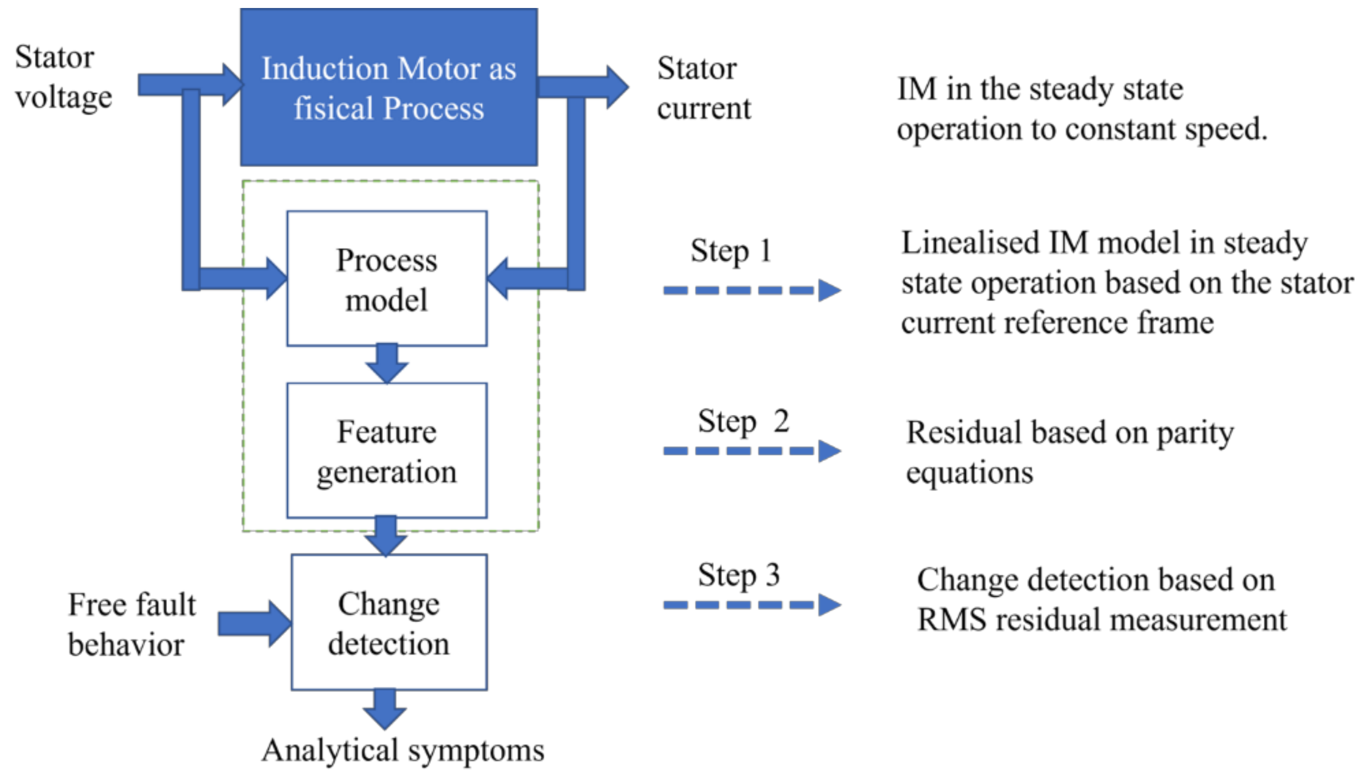
4. Fault Diagnosis Based on Stator Current Reference Frame

Once the vectors and matrices concerned from (30) are identified, the method of parity equations is applied, which initially consists of calculating the T matrix defined in (5) where A and C are obtained from (31) and (33), respectively. Then T and Q_u are given as:

$$T=\left[\begin{array}{c}C\\ C·A\\ C·A^2\end{array}\right]=\left[\begin{array}{ccc}& \begin{array}{ccc}1& 0& 0\\ 0& 1& 0\\ 0& 0& 1\end{array}& \\ -\frac{A1R_{sa}}{k1}& -\frac{A2R_{sb}}{k1}& -\frac{A3R_{sc}}{k1}\\ -\frac{A2R_{sa}}{k1}& -\frac{A5R_{sb}}{k1}& -\frac{A6R_{sc}}{11}\\ -\frac{A3R_{sa}}{k1}& -\frac{A6R_{sb}}{k1}& -\frac{A9R_{sc}}{k1}\\ & \begin{array}{ccc}{C{A}^2}_{11}& {C{A}^2}_{12}& {C{A}^2}_{13}\\ {C{A}^2}_{21}& {C{A}^2}_{22}& {C{A}^2}_{23}\\ {C{A}^2}_{31}& {C{A}^2}_{32}& {C{A}^2}_{33}\end{array}& \end{array}\right]$$

(34)

$$Q_u=\left[\begin{array}{ccc}0& 0& 0\\ C B& 0& 0\\ C A B& C B& 0\end{array}\right]=\left[\begin{array}{ccc}\begin{array}{cc}0& 0\\ 0& 0\end{array}& \begin{array}{cc}0& 0\\ 0& 0\end{array}& \begin{array}{cc}0& 0\\ 0& 0\end{array}\\ \begin{array}{cc}\frac{1}{L_{sa}}& 0\\ 0& 0\end{array}& \begin{array}{cc}0& 0\\ 0& 0\end{array}& \begin{array}{cc}0& 0\\ 0& 0\end{array}\\ \begin{array}{cc}\frac{R_{sa}}{L_{sa}{}^2}& 0\\ \frac{K_f N_p}{J L_{sa}}& 0\end{array}& \begin{array}{cc}\frac{1}{L_{sa}}& 0\\ 0& 0\end{array}& \begin{array}{cc}0& 0\\ 0& 0\end{array}\end{array}\right]$$

(35)

Now, considering a system with no disturbances and no external faults, it is necessary that a matrix W that fulfills the condition $w^T T=0$ to ensure that the parity space if the vectors of $W$ are linearly independent. A procedure to find the matrix $W$ is to analyze separately the rows of $W$ that multiply the matrix $T$ and ensure the null space. For this case, it must be considered that the matrix T has a range of 9 × 3, so the range of W can be 3 × 9 in the following way, which will allow us to subsequently obtain three residuals.

$$\begin{gathered} \mathrm{W}=\left[\begin{array}{ccc}w{1}^T& w{2}^T& w{3}^T\end{array}\right]=\left[\begin{array}{ccc}\mathrm{w}11& \mathrm{w}21& \mathrm{w}31\\ \mathrm{w}12& \mathrm{w}22& \mathrm{w}32\\ \mathrm{w}13& \mathrm{w}23& \mathrm{w}33\end{array}\right]= \\ \left[\begin{array}{ccccccccc}w{11}_1& w{11}_2& w{11}_3& w{21}_1& w{21}_2& w{21}_3& w{31}_1& w{31}_2& w{31}_3\\ w{12}_1& w{12}_2& w{12}_3& w{22}_1& w{22}_2& w{22}_3& w{32}_1& w{32}_2& w{33}_3\\ w{13}_1& w{13}_2& w{13}_3& w{23}_1& w{23}_2& w{23}_3& w{33}_1& w{33}_2& w{33}_3\end{array}\right] \end{gathered}$$

(36)

According to the position of the matrices $W$ and T, it can be separated by rows as follows

$$\begin{gathered} w{1}^T·\mathrm{C}+w{2}^T·\mathrm{C} \mathrm{A}+w{3}^T·{\mathrm{C} \mathrm{A}}^2=0 \\ \mathrm{or} \\ \mathrm{w}11·\mathrm{C}+\mathrm{w}21·\mathrm{CA}+\mathrm{w}31·{\mathrm{CA}}^2=0 \\ \mathrm{w}12·\mathrm{C}+\mathrm{w}22·\mathrm{CA}+\mathrm{w}32·{\mathrm{CA}}^2=0 \\ \mathrm{w}13·\mathrm{C}+\mathrm{w}23·\mathrm{CA}+\mathrm{w}33·{\mathrm{CA}}^2=0 \end{gathered}$$

(37)

For this case, it is necessary to find three equations to isolate the faults per phase, so $w3i·C{A}^2$ must be neglected making $w{3}^T=0$ or w31 = w32 = w33 = 0. Furthermore, it is observed that the matrix C is unitary and then the expression is reduced as:

$$\begin{gathered} w{1}^T=-w{2}^T·\mathrm{A} \\ \mathrm{or} \\ \mathrm{w}11=-w21·\mathrm{A} \\ \mathrm{w}12=-w22·\mathrm{A} \\ \mathrm{w}13=-w23·\mathrm{A} \end{gathered}$$

(38)

Now, the task is to find w11, w12, w31 or w21, w22, w23 that satisfies $W T=0$ and, at the same time, determine the fault isolation per phase in the residual equation r(t) expressed in (13). For this case study, we found that the following $w{1}^T$ is the best simplified proposal to detect and isolate faults per phase.

$$\mathrm{W}{1}^{\mathrm{T}}=\left[\begin{array}{ccc}0& R_{sb}& R_{sc}\\ R_{sa}& 0& R_{sc}\\ R_{sa}& R_{sb}& 0\end{array}\right]$$

(39)

Then

$$\mathrm{w}{2}^{\mathrm{T}}=-\frac{\mathrm{w}{1}^{\mathrm{T}}}{\mathrm{A}}$$

Collecting terms and simplifying for W

$$\mathrm{W}=\left[\begin{array}{ccccccccc}0& R_{sb}& R_{sc}& -m_{sr}& (L_{sb}+\frac{m_{sr}}{2})& (L_{sc}+\frac{m_{sr}}{2})& 0& 0& 0\\ R_{sa}& 0& R_{sc}& (L_{sa}+\frac{m_{sr}}{2})& -m_{sr}& (L_{sc}+\frac{m_{sr}}{2})& 0& 0& 0\\ R_{sa}& R_{sb}& 0& (L_{sa}+\frac{m_{sr}}{2})& (L_{sb}+\frac{m_{sr}}{2})& -m_{sr}& 0& 0& 0\end{array}\right]$$

(40)

Then, the residual set obtained for this general case study is

$$r\left(t\right)=W Y\left(t\right)-W{Q}_{u}U\left(t\right)$$

$$\begin{gathered} r_5\left(t\right)=R_{sb} I_{sb}\left(t\right)+L_{sb}\frac{d}{dx}\left[I_{sb}\left(t\right)\right]+0.5 m_{sr}\frac{d}{dx}\left[I_{sb}\left(t\right)\right]-V_{sb}\left(t\right)+R_{sc} I_{sc}\left(t\right) \\ +L_{sc}\frac{d}{dx}\left[I_{sc}\left(t\right)\right]+0.5 m_{sr}\frac{d}{dx}\left[I_{sc}\left(t\right)\right]-V_{sc}\left(t\right)-m_{sr}\frac{d}{dx}\left[I_{sa}\left(t\right)\right] \\ {r}_6\left(t\right)=R_{sa} I_{sa}\left(t\right)+L_{sa}\frac{d}{dx}\left[I_{sa}\left(t\right)\right]+0.5 m_{sr}\frac{d}{dx}\left[I_{sa}\left(t\right)\right]-V_{sa}\left(t\right)+R_{sc} I_{sc}\left(t\right) \\ +L_{sc}\frac{d}{dx}\left[I_{sc}\left(t\right)\right]+0.5 m_{sr}\frac{d}{dx}\left[I_{sc}\left(t\right)\right]-V_{sc}\left(t\right)-m_{sr}\frac{d}{dx}\left[I_{sb}\left(t\right)\right] \\ {r}_7\left(t\right)=R_{sa} I_{sa}\left(t\right)+L_{sa}\frac{d}{dx}\left[I_{sa}\left(t\right)\right]+0.5 m_{sr}\frac{d}{dx}\left[I_{sa}\left(t\right)\right]-V_{sa}\left(t\right)+R_{sb} I_{sb}\left(t\right) \\ +L_{sb}\frac{d}{dx}\left[I_{sb}\left(t\right)\right]+0.5 m_{sr}\frac{d}{dx}\left[I_{sb}\left(t\right)\right]-V_{sb}\left(t\right)-m_{sr}\frac{d}{dx}\left[ I_{sc}\left(t\right)\right] \end{gathered}$$

(41)

Now, using the residual set above it, it is possible to identify the failure phase in $R_{si}$, $V_{si}$ and $L_{si}$ it, although in $I_{si}$ is not possible (see

Table 2. Fault detection matrix in the stator current reference frame: (a) Unsimplified residual set with derivative terms, (b) Simplified residual set without derivative terms.

(a)
	Faults		${\mathrm{r}}_5$	${\mathrm{r}}_6$	${\mathrm{r}}_7$
Parametric	Rs	Rsa	0	I	I
		Rsb	I	0	I
		Rsc	I	I	0
	Ls	Lsa	0	I	I
		Lsb	I	0	I
		Lsc	I	I	0
		msr	I	I	I
Additive	Is	Isa	I	I	I
		Isb	I	I	I
		Isc	I	I	I
	Vs	Vsa	0	I	I
		Vsb	I	0	I
		Vsc	I	I	0
(b)
	Faults		${\mathrm{r}}_5$	${\mathrm{r}}_6$	${\mathrm{r}}_7$
Parametric	Rs	Rsa	0	I	I
		Rsb	I	0	I
		Rsc	I	I	0
	Ls	Lsa	0	0	0
		Lsb	0	0	0
		Lsc	0	0	0
		msr	0	0	0
Additive	Is	Isa	0	I	I
		Isb	I	0	I
		Isc	I	I	0
	Vs	Vsa	0	I	I
		Vsb	I	0	I
		Vsc	I	I	0

“I” represents change positive or negative.

). In this case, theoretically, derivatives involved should not be ignored because there are no DC components, as in the previous DQ model [13]. However, heuristically, the magnitudes of the derivative terms can be neglected with respect to the magnitudes of the remaining terms, which involve the signals from voltage and current sensors and, finally, the residual set is simplified as follows. So, the fault diagnosis matrix allows us to detect the failure phase of $I_s$, but the fault detection of $L_s$ is lost.

$$\begin{gathered} r_5\left(t\right)=R_{sb} I_{sb}\left(t\right)-V_{sc}\left(t\right)-V_{sb}\left(t\right)+R_{sc} I_{sc}\left(t\right) \\ {r}_6\left(t\right)=R_{sa} I_{sa}\left(t\right)-V_{sc}\left(t\right)-V_{sa}\left(t\right)+R_{sc} I_{sc}\left(t\right) \\ {r}_7\left(t\right)=R_{sa} I_{sa}\left(t\right)-V_{sb}\left(t\right)-V_{sa}\left(t\right)+R_{sb} I_{sb}\left(t\right) \end{gathered}$$

(42)

Note that, $R_{si}$, $L_{si}$, $I_{si}$, and $V_{si}$ have the same signature, but in combination with the fault detection using DQ reference frame it is possible to fully identify the affected parameter, as shown in

Table 3. Full fault detection matrix using DQ and Three-phase model for fault diagnosis.

DQ Model							Three-Phase Model
Fault			${\mathrm{r}}_1$	${\mathrm{r}}_2$	${\mathrm{r}}_3$	${\mathrm{r}}_4$	${\mathrm{r}}_5$	${\mathrm{r}}_6$	${\mathrm{r}}_7$
Parametric	${\mathrm{R}}_{\mathrm{s}}$	${\mathrm{R}}_{\mathrm{sa}}$	I	0	0	I	0	I	I
		${\mathrm{R}}_{\mathrm{sb}}$	I	0	0	I	I	0	I
		${\mathrm{R}}_{\mathrm{sc}}$	I	0	0	I	I	I	0
		${\mathrm{R}}_{\mathrm{r}}$	I	0	0	I	0	I	I
	${\mathrm{L}}_{\mathrm{s}}$	${\mathrm{L}}_{\mathrm{sa}}$	I	0	I	I	I	I	I
		${\mathrm{L}}_{\mathrm{sb}}$	I	0	I	I	I	I	I
		${\mathrm{L}}_{\mathrm{sc}}$	I	0	I	I	I	I	I
		${\mathrm{L}}_{\mathrm{r}}$	I	I	I	I	I	I	0
		$\mathrm{B}$	0	I	I	I	0	0	0
		${\mathrm{B}}_{\mathrm{l}}$	0	I	I	I	0	0	0
Additive	${\mathrm{I}}_s$	${\mathrm{I}}_{sa}$	I	I	I	0	0	I	I
		${\mathrm{I}}_{sb}$	I	I	I	0	I	0	I
		${\mathrm{I}}_{sc}$	I	I	I	0	I	I	0
		${\mathsf{\omega }}_{\mathrm{r}}$	I	I	0	I	0	0	0
	${\mathrm{V}}_{\mathrm{s}}$	${\mathrm{V}}_{\mathrm{sa}}$	I	0	I	I	0	I	I
		${\mathrm{V}}_{\mathrm{sa}}$	I	0	I	I	I	0	I
		${\mathrm{V}}_{\mathrm{sa}}$	I	0	I	I	I	I	0

“I” represents change positive or negative.

.

It can also be noted from Table 2 that the fault diagnosis matrix with derivative terms cannot distinguish the fault between $L_s$ and $V_s$, although it is possible to identify the damaged phase. This is a problem of the DQ detection model [13]. However, when the fault diagnosis matrix without derivative terms is considered, the detection range is increased. For example, fault detection on $V_s$ is isolated and fault detection on $I_s$ is added, although fault detection in $L_s$ is lost (see Table 2).

The logical evaluation of the residual set can be easily carried out using the effective value or RMS value per cycle for each residual signal and compensate the steady state errors attributed to the proposed linearized fault diagnosis model based on the stator current reference frame. Another important point to consider in an experimental way is the detection of the zero crossing of the residual signals before the evaluation of the RMS value per cycle.

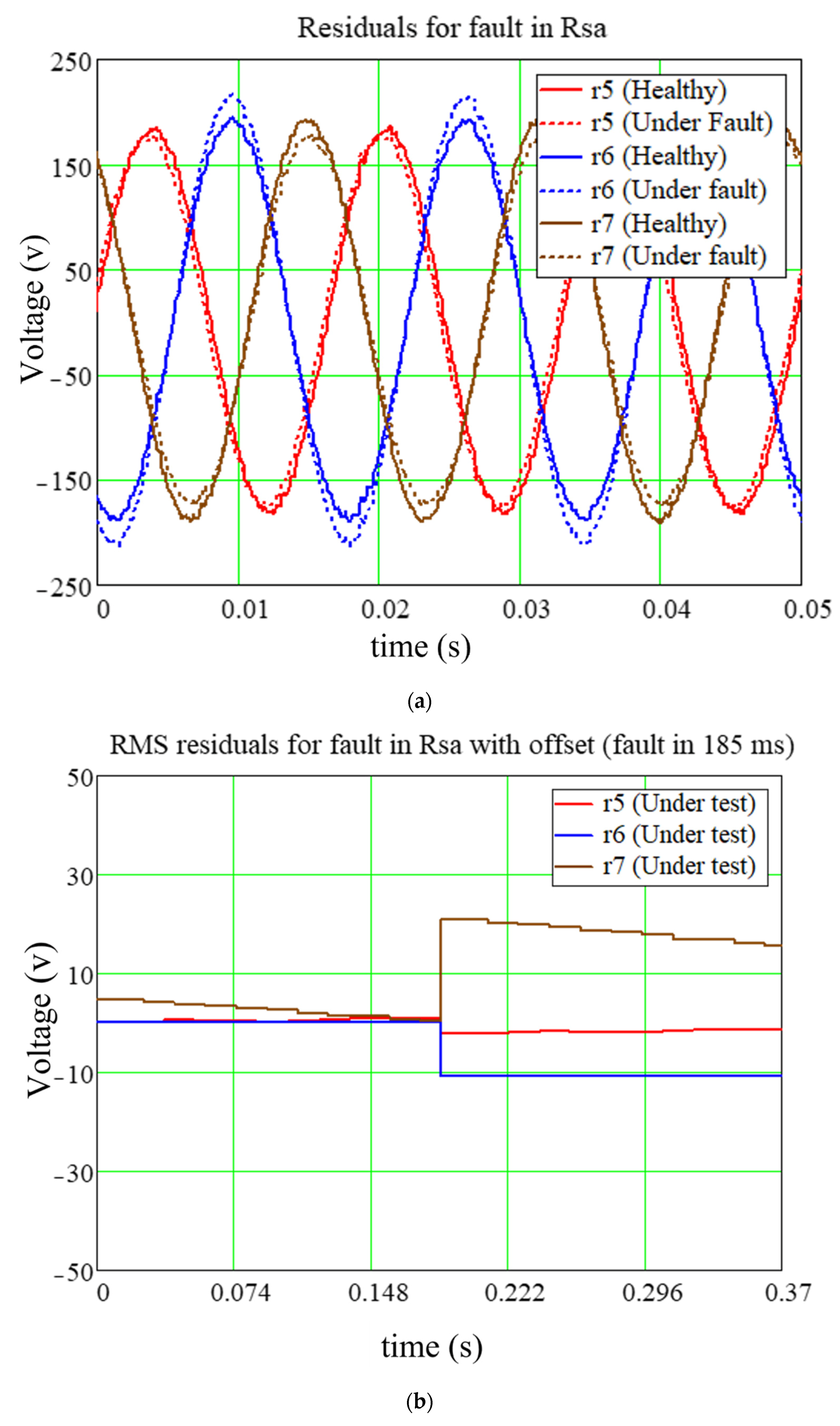
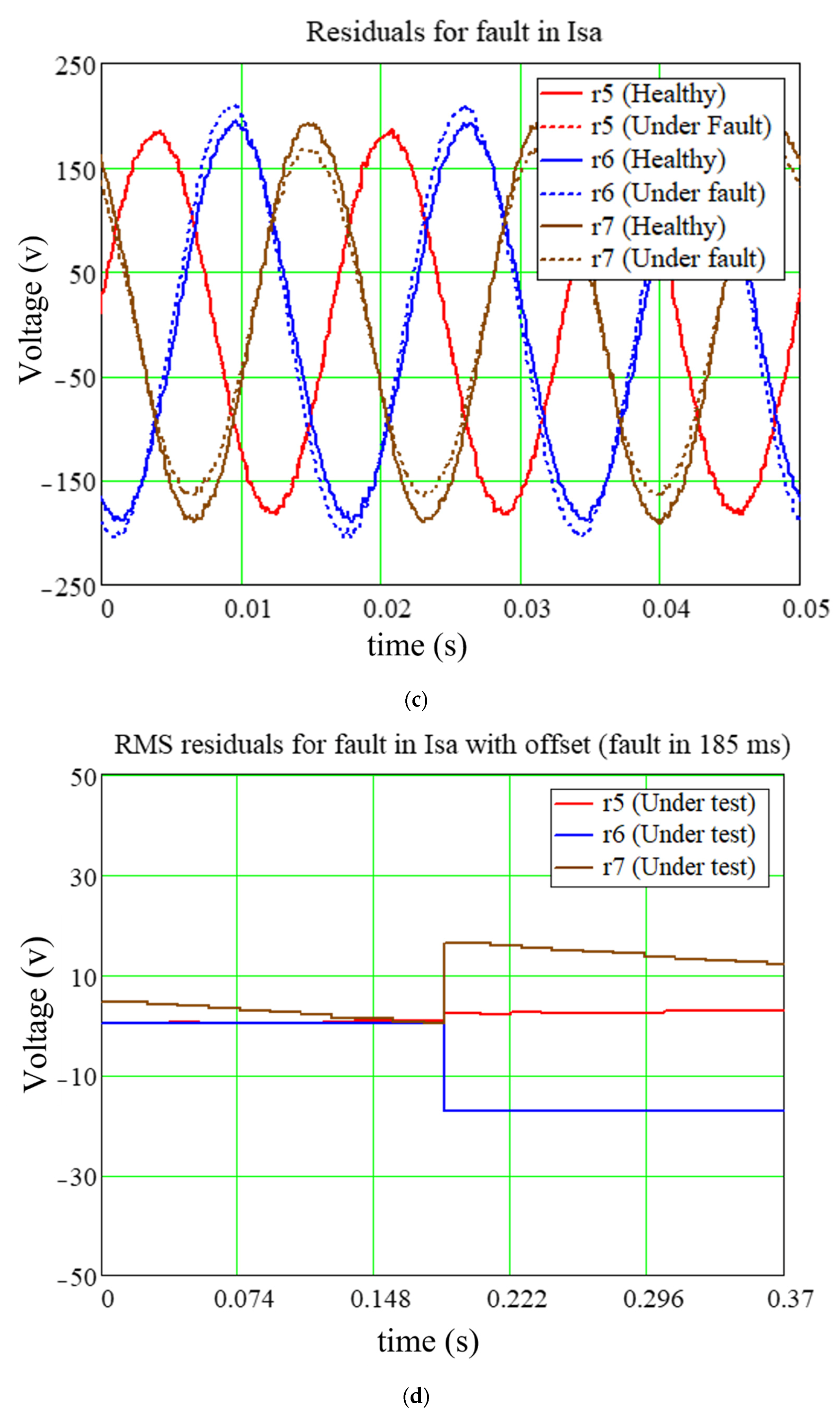
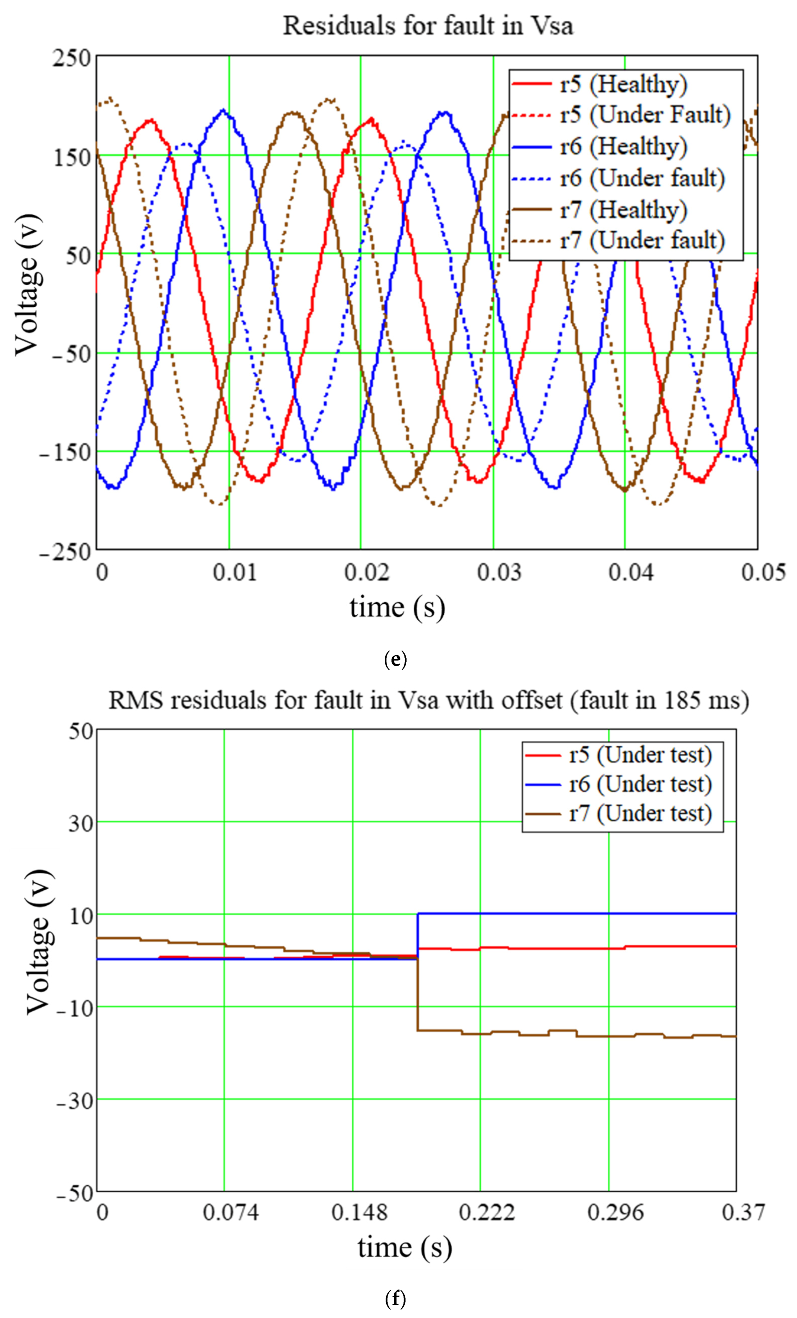
5. Discussion and Results

The simulation schematic in Figure 3 shows the full fault diagnosis system using the blocks based on the DQ reference frame and based on the stator current reference frame, which has its diagnosis matrix represented in Table 3. In this work we only focus on the complementary fault diagnosis block based on the stator current reference frame. Regarding the simplified Equation (42), the failure analysis using experimental and simulation tests focus on $R_s$, $I_s$ and $V_s$ (particularly for phase a).

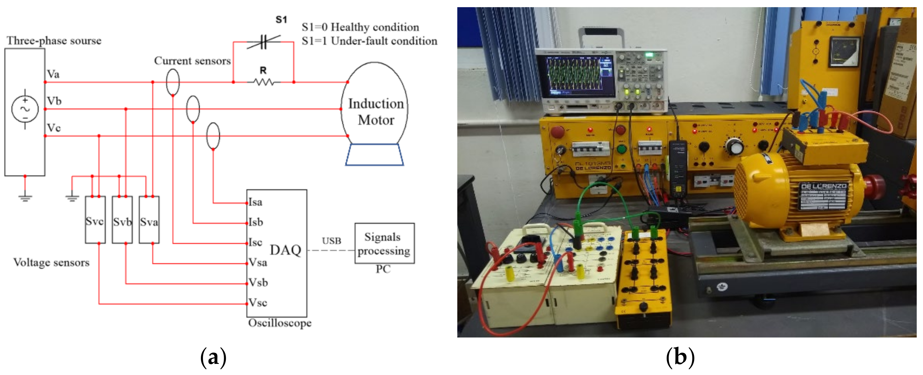
5.1. Fault Detection Scheme for Experimental and Simulation Setup

Figure 3 shows the simulation scheme to emulate the parametric fault in the stator resistance. In this case, for the fault in $R_{sa}$, when t < 1.5 s, the switch S1 is enabled for the fault-free case, when t > 1.5 s, the switch S1 is disabled, and a resistance R is added to the stator resistance and the under-fault case is generated.

Figure 4 shows the experimental scheme to emulate the stator resistance fault in $R_{sa}$. A instrumental block diagram to measure $I_s$ and $V_s$ in healthy and under-fault conditions is shown in Figure 4a. Regarding a practical point of view, using only one current probe and only one voltage differential probe, triggering with a voltage phase, in this case $V_{sa}$, is a good practical tip, since the uncertainty and unbalance of the measurement, attributed to the calibration of the current and voltage sensors, is reduced. Figure 4b shows the experimental setup for this case and the signals set measured with the oscilloscope and stored in USB memory are subsequently processed using a mathematical software which calculates the original and compensated-RMS residual set, as shown in Figure 6, respectively. The fault transient in $R_s$, $I_s$ and $V_s$ for phases b,c are omitted to simplify the residual experimental test.

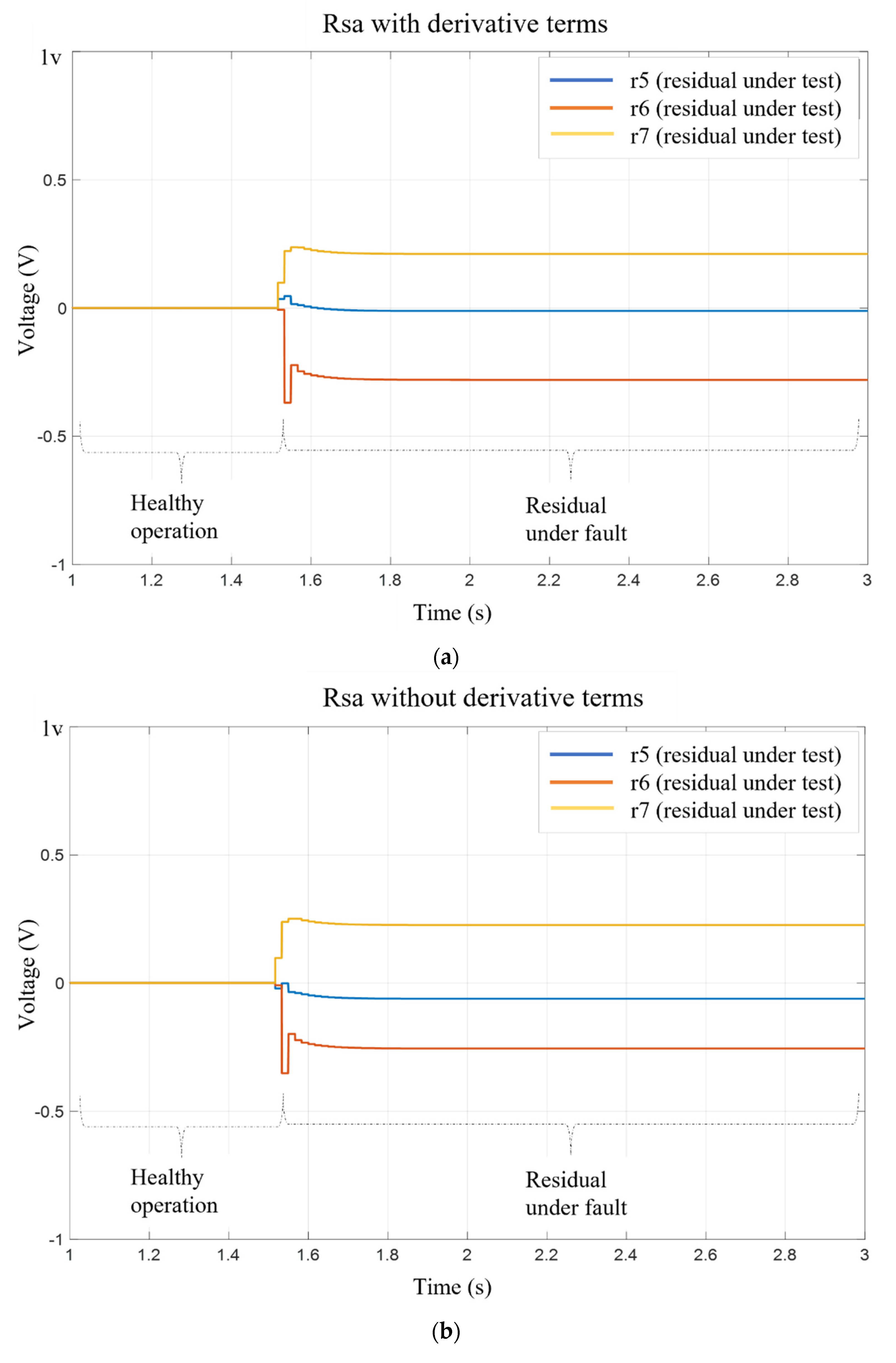
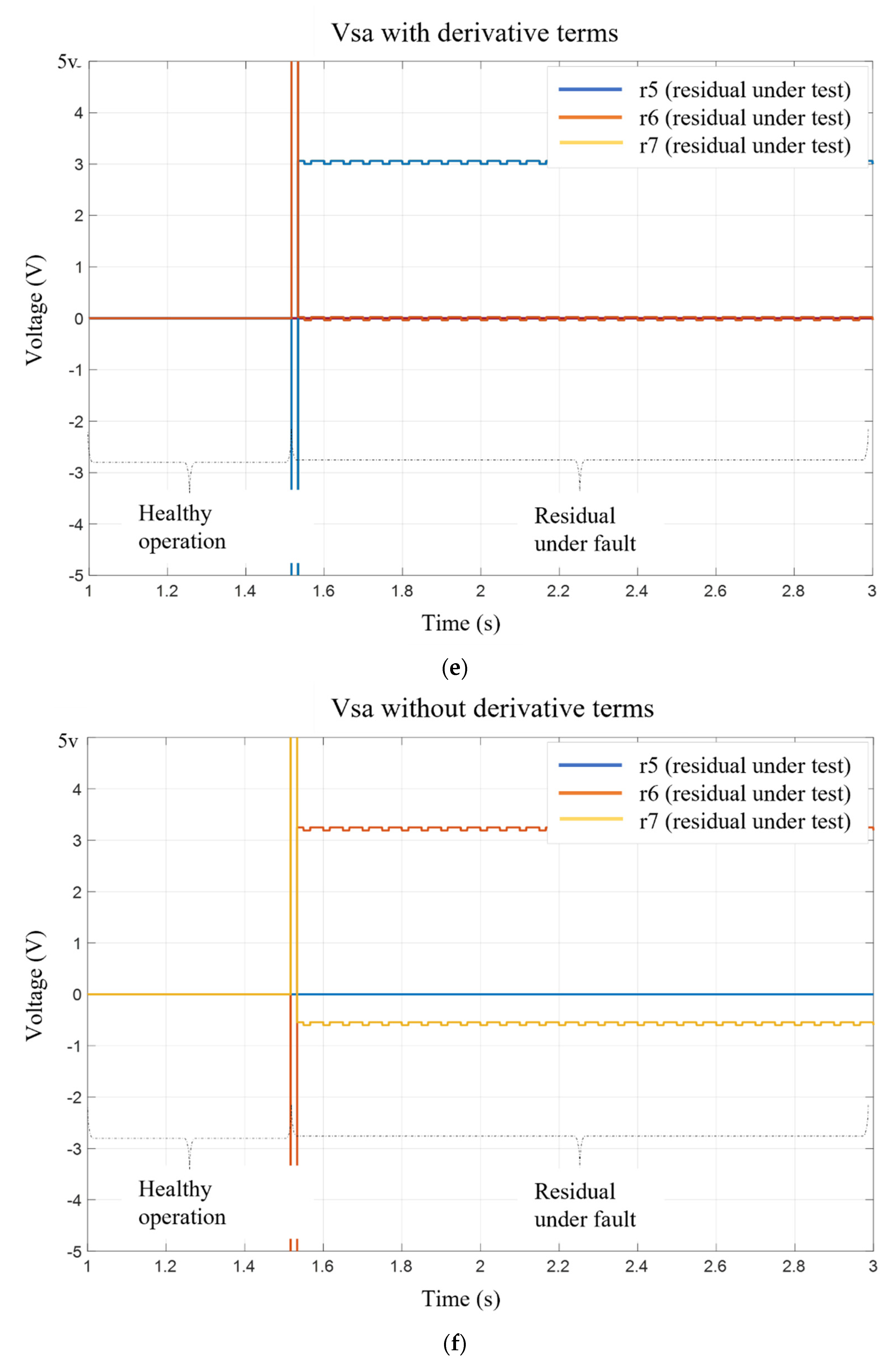
5.2. Fault Analysis for Experimental and Simulation Test

Simulation and experimental results of the residual set (r5, r6 and r7) with compensated RMS value in healthy and under-fault conditions are shown in Figure 5 and Figure 6, respectively. Figure 5a,b show the simulation residual transient in healthy and under-fault condition for $R_{sa}$, using the equations obtained in (41) and (42), respectively. Figure 6a,c,e show the residual signal before compensation RMS value, using the simplified Equation (42) in healthy and under-fault condition.

Regarding the sensor faults, similarly to the previous case, in Figure 5c–e a pair of switches are used to generate additive faults in the current and voltage sensors $I_{sa}$ and $V_{sa}$, respectively. That is, at t < 1.5 s, the healthy condition is carried out and at t > 1.5 s, a new connection path is generated to provide a zero value in the current or voltage input of the fault detection block based on the stator current reference frame, which uses the equations in (41) and (42), respectively.

Figure 5 and Figure 6b,d,f show the simulation and experimental results using the simplified equation proposed. Likewise, the trends consistent with the proposed fault diagnosis matrix of Table 2b regarding fault in $R_{sa}$, $I_{sa}$, or $V_{sa}$ is observed. The different magnitude is due to the use of motors of different power for both the simulation and experimental tests. In this way, for larger capacity motors, as in this experimental case, the magnitudes of the residues are larger and therefore the measurement in the diagnosis system is easier. It should not be forgotten that the proposed system complements the scheme developed in [13], which allows identifying the affected phase if the fault is $R_s$, $I_s$ or $V_s$.

Regarding the experimental test of Figure 6b,d,f, a smoothed fault transient is shown when the fault appears in t = 185 ms. It is important to mention that the fault transient during the fault-free to under-fault case of Figure 6b,d,f is omitted because the measurements were made during the steady state operation of the residue. which does not apply to the simulation results of Figure 5. On the other hand, the manufacturing imbalance of both the induction motor and the source AC generator, used in the experimental tests, causes non-symmetrical phases and therefore non-constant residuals. Additionally, data used with long sampling periods and forced triggering in single mode, cause a shift in the signals at the extremes of the synchronization, which are manifested in non-symmetrical and non-constant values during the residual or RMS calculation, respectively.

In the simulation and experimental tests an IM of 0.5 HP and 1.5 HP was used, respectively. The main idea was to check the similar trend of the residuals, as shown in Figure 5 and Figure 6.

6. Conclusions

The IM modeling for fault diagnosis using the parity equation has, as its main assumption, the steady state behavior of three-phase induction motor. In this way, it is convenient to consider, heuristically, a fault diagnosis dead time at start-up according to the stabilization time. Regarding the fault diagnosis for IM in the DQ reference frame, the obtained result allows us to detect electrical and mechanical faults because the IM model deduced is matched to the DC motor model, so the existence of parity space is achieved. However, the isolation of the phase corresponding to the damaged parameter is not obtained due to the DQ transformation. Now, with respect to fault diagnosis for IM in stator current reference frame, the residual obtained only allows to detect the damage phase without determining the damaged parameter. Then, the two previous reference frames are used to generate a full detection matrix. Finally, the simplified residual set obtained in this work is very simple to implement in any digital processor, since the operators are addition, subtraction, and multiplication without recursion. Nevertheless, the fault detection in $L_s$ is lost. On the other hand, the unsimplified residual set is more complex and the fault detection in $I_s$ is lost, but the detection of $L_s$ is obtained. The fault detection in current sensors is slightly affected and fault magnitudes in $L_s$ are almost negligible. Maybe, the main problem of the full fault diagnosis system is that the parameters of the IM must be known a priori, and false alarms attributed to load changes occur. So future work aims to add robustness to load and input-signal variations through adaptive thresholds in the decision block.

References

1. Bianchini, C.; Immovilli, F.; Cocconcelli, M.; Rubini, R.; Bellini, A. Fault Detection of Linear Bearings in Brushless AC Linear Motors by Vibration Analysis. IEEE Trans. Ind. Electron. 2011, 58, 1684–1694. [Google Scholar] [CrossRef]
2. Kolla, S.; Varatharasa, L. Identifying three-phase induction motor faults using artificial neural networks. ISA Trans. 2000, 39, 433–439. [Google Scholar] [CrossRef]
3. Nandi, S.; Toliyat, H.A.; Li, X. Condition Monitoring and Fault Diagnosis of Electrical Motors—A Review. IEEE Trans. Energy Convers. 2005, 20, 719–729. [Google Scholar] [CrossRef]
4. Loparo, K.; Adams, M.; Lin, W.; Abdel-Magied, M.; Afshari, N. Fault detection and diagnosis of rotating machinery. IEEE Trans. Ind. Electron. 2000, 47, 1005–1014. [Google Scholar] [CrossRef]
5. Mendes, A.; Cardoso, A.J.M. Fault-Tolerant Operating Strategies Applied to Three-Phase Induction-Motor Drives. IEEE Trans. Ind. Electron. 2006, 53, 1807–1817. [Google Scholar] [CrossRef]
6. Cash, M.; Habetler, T.; Kliman, G. Insulation failure prediction in AC machines using line-neutral voltages. IEEE Trans. Ind. Appl. 1998, 34, 1234–1239. [Google Scholar] [CrossRef]
7. Klima, J. Analytical investigation of an induction motor drive under inverter fault mode operations. IEE Proc.-Electr. Power Appl. 2003, 150, 255–262. [Google Scholar] [CrossRef]
8. Chan, C.; Hua, S.; Hong-Yue, Z. Application of Fully Decoupled Parity Equation in Fault Detection and Identification of DC Motors. IEEE Trans. Ind. Electron. 2006, 53, 1277–1284. [Google Scholar] [CrossRef] [Green Version]
9. Bouattour, J. Diagnosing Parametric Faults in Induction Motors with Nonlinear Parity Relations. IFAC Proc. Vol. 2000, 33, 971–976. [Google Scholar] [CrossRef]
10. Isermann, R. Model base fault detection and diagnosis methods. In Proceedings of the American Control Conference, Seattle, WA, USA, 21–23 June 1995; Volume 3. [Google Scholar] [CrossRef]
11. Isermann, R. Supervision, fault-detection and fault-diagnosis methods—An introduction. Control Eng. Pract. 1997, 5, 639–652. [Google Scholar] [CrossRef]
12. Rodriguez, M.; Hernandez, M.; Mendez, F.; Sibaja, P.; Hernandez, L. A simple fault detection of induction motor by using parity equations. In Proceedings of the SDEMPED 2011-8th IEEE Symposium on Diagnostics for Electrical Machines, Power Electronics and Drives, Bologna, Italy, 5–8 September 2011; pp. 573–579. [Google Scholar] [CrossRef]
13. Chulines, E.; Rodríguez, M.A.; Duran, I.; Sánchez, R. Simplified Model of a Three-Phase Induction Motor for Fault Diagnostic Using the Synchronous Reference Frame DQ and Parity Equations. In Proceedings of the 2nd IFAC Conference on Modelling, Identification and Control of Nonlinear Systems MICNON 2018, Jalisco, Mexico, 20–22 June 2018; Volume 51. [Google Scholar] [CrossRef]
14. El Khil, S.K.; Jlassi, I.; Estima, J.; Mrabet-Bellaaj, N.; Cardoso, A.M. Current sensor fault detection and isolation method for PMSM drives, using average normalised currents. Electron. Lett. 2016, 52, 1434–1436. [Google Scholar] [CrossRef]
15. Gertler, J.J. Fault Detection and Diagnosis in Engineering Systems, 1st ed.; CRC Press: Boca Raton, FL, USA, 2017; Volume 1. [Google Scholar] [CrossRef]
16. Isermann, R. Fault-Diagnosis Systems: An Introduction from Fault Detection to Fault Tolerance, 1st ed.; Springer: Berlin/Heidelberg, Germany; New York, NY, USA, 2006; ISBN 978-3-540-24112-6. [Google Scholar]
17. Kazmierkowski, M.P. Electric motor drives: Modeling, analysis and control. Int. J. Robust Nonlinear Control 2004, 14, 767–769. [Google Scholar] [CrossRef]
18. Höfling, T.; Isermann, R. Fault detection based on adaptive parity equations and single-parameter tracking. Control Eng. Pract. 1996, 4, 1361–1369. [Google Scholar] [CrossRef]
19. Rodríguez, M.A.; Hernandez, M.; Golikov, V.; Martínez, G. Fault Diagnostic Based on Parity Equations Applied to Induction Motor. In Proceedings of the XXI Congreso de la Asociación Chilena de Control Automático ACCA, Santiago, Chile, 5–7 November 2014; pp. 65–71. [Google Scholar]
20. Krause, P.; Wasynczuk, O.; Sudhoff, S.; Pekarek, S. Analysis of Electric Machinery and Drive Systems, 1st ed.; IEEE: New York, NY, USA, 2013; Volume 1, ISBN 9781118024294. [Google Scholar] [CrossRef]
Figure 1. Model-based fault detection scheme for IM working in the steady state to constant speed.
Machines 10 00379 g001
Figure 2. Continuous time model in state spaces based on parity equations.
Machines 10 00379 g002
Figure 3. Full residual simulation scheme using DQ and stator current reference frame.
Machines 10 00379 g003
Figure 4. Experimental scheme to emulate stator resistor fault: (a) Block diagram of the experimental setup, (b) Image of the experimental setup.
Machines 10 00379 g004
Figure 5. Residual simulation test: (a) Fault in Rsa using derivative terms, (b) Fault in Rsa without derivative terms, (c) Fault in Isa using derivative terms, (d) Fault in Isa without derivative terms, (e) Fault in Vsa using derivative terms, (f) Fault in Vsa without derivative terms.
Machines 10 00379 g005aMachines 10 00379 g005bMachines 10 00379 g005c
Figure 6. Residual experimental test using the simplified equation: (a) Original residual measurement with healthy and under-fault R s a , (b) Compensated-RMS residual measurement with healthy and under-fault R s a , (c) Original residual measurement with healthy and under-fault I s a , (d) Compensated-RMS residual measurement with healthy and under-fault I s a , (e) Original residual measurement with healthy and under-fault V s a , (f) Compensated-RMS residual measurement with healthy and under-fault V s a .
Machines 10 00379 g006aMachines 10 00379 g006bMachines 10 00379 g006c