
Bearing Faulty Prediction Method Based on Federated Transfer Learning and Knowledge Distillation


Abstract
:1. Introduction
- (1)
- The training process of the traditional deep learning model requires large amounts of labeled data; however, in the practical industry, it is extremely costly to acquire labeled data, especially the labeled data representing the machine faulty condition which is usually not well preserved.
- (2)
- Since the traditional deep learning model is usually trained on large amounts of historical datasets, the model training process is usually time consuming due to its large training data volumes. How to accelerate the training process of the faulty prediction model remains a challenge.
- (1)
- The performance of the traditional transfer learning model relies on the quality of the source data and the degree of similarity between the source domain and the target domain which poses limitations on the generalization ability of the transfer learning model. How to construct a generalized transfer learning framework that is applicable to different transfer learning tasks remains a great challenge.
- (2)
- With the increase in the transferred features and parameters from the original model which contains “knowledge” from different but related source domains, the parameter scale of the transfer learning model can be very large, causing difficulties for the model field deployment. How to release the parameter size of the transfer learning model remains a topic of consideration.
- (1)
- Dealing with the first issue listed above, several cumbersome models are set up through offline training on multiple related source domain datasets. Thus, containing prior knowledge of different source domain datasets;
- (2)
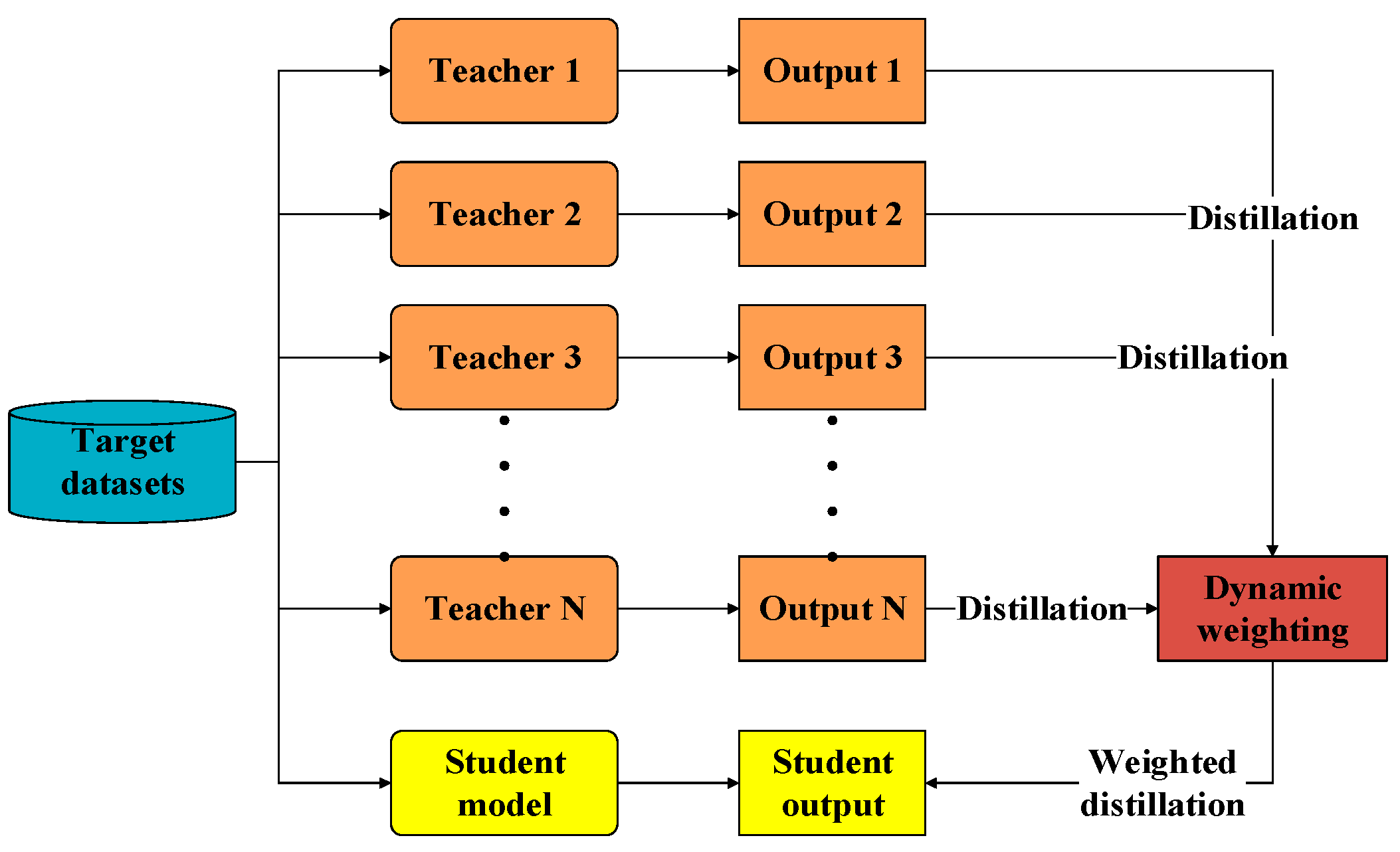
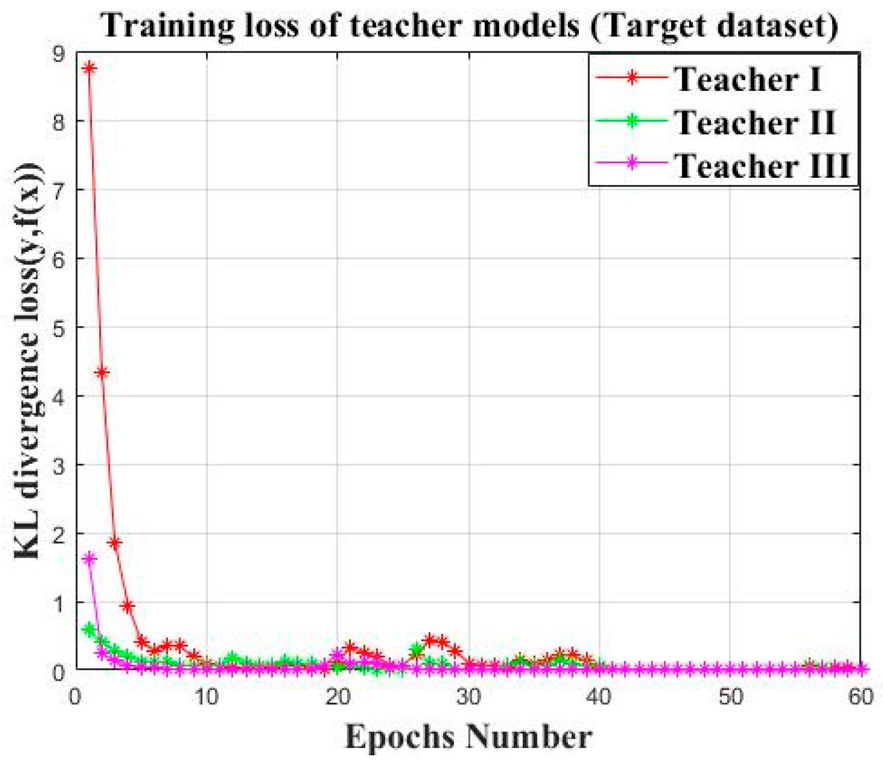
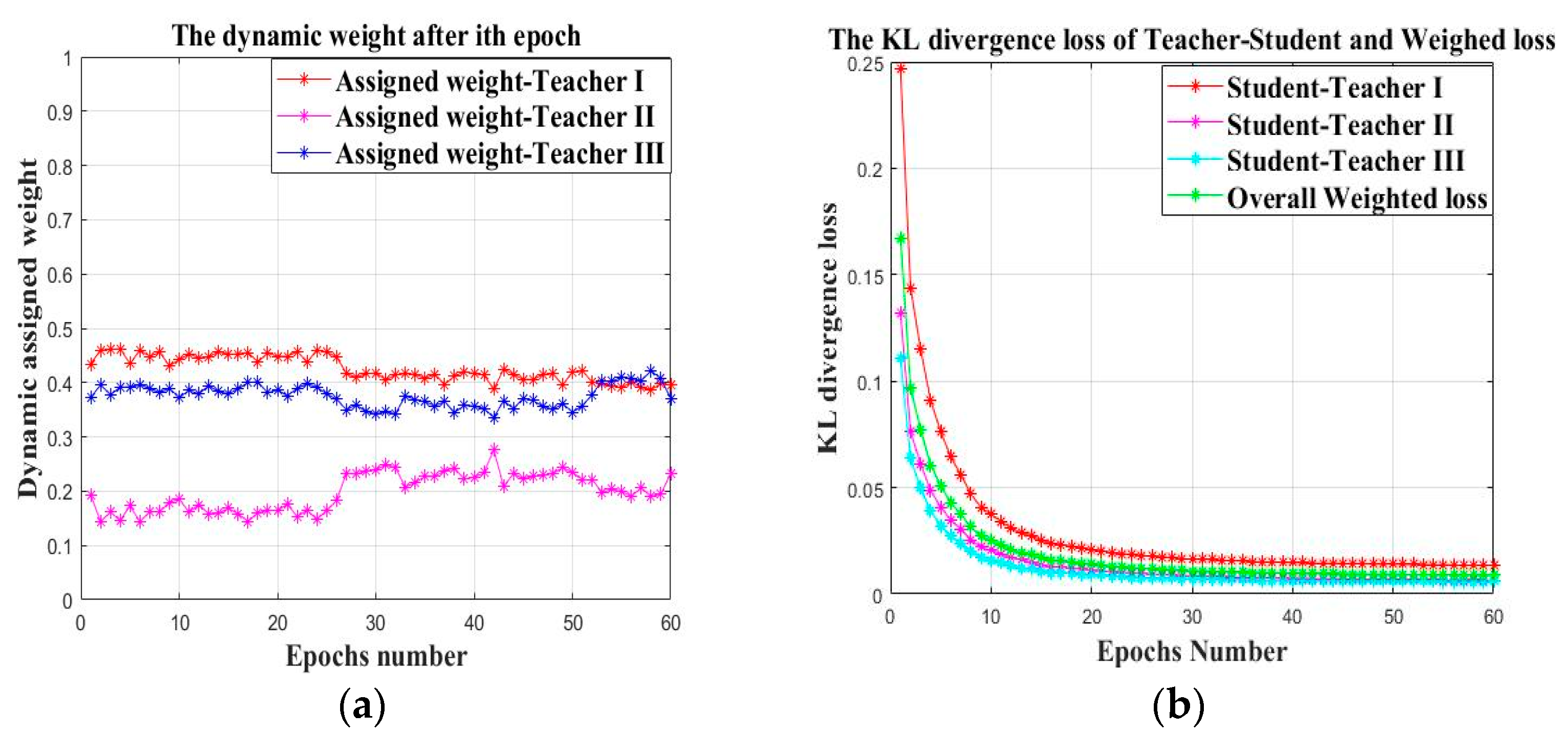
- Dealing with the second issue listed above, the cumbersome models pretrained on multiple different but related datasets are used as teacher models during the joint training process with the student model on the target datasets. This is also called knowledge distillation. The established teacher models can promote the training efficiency of the shallow structured student model while maintaining its small parameter size by using the knowledge distillation. The assigned weights of the teacher models are dynamically changed during the joint training process based on the real time KL-divergence loss between the corresponding teacher output and the true label.
2. Related Work
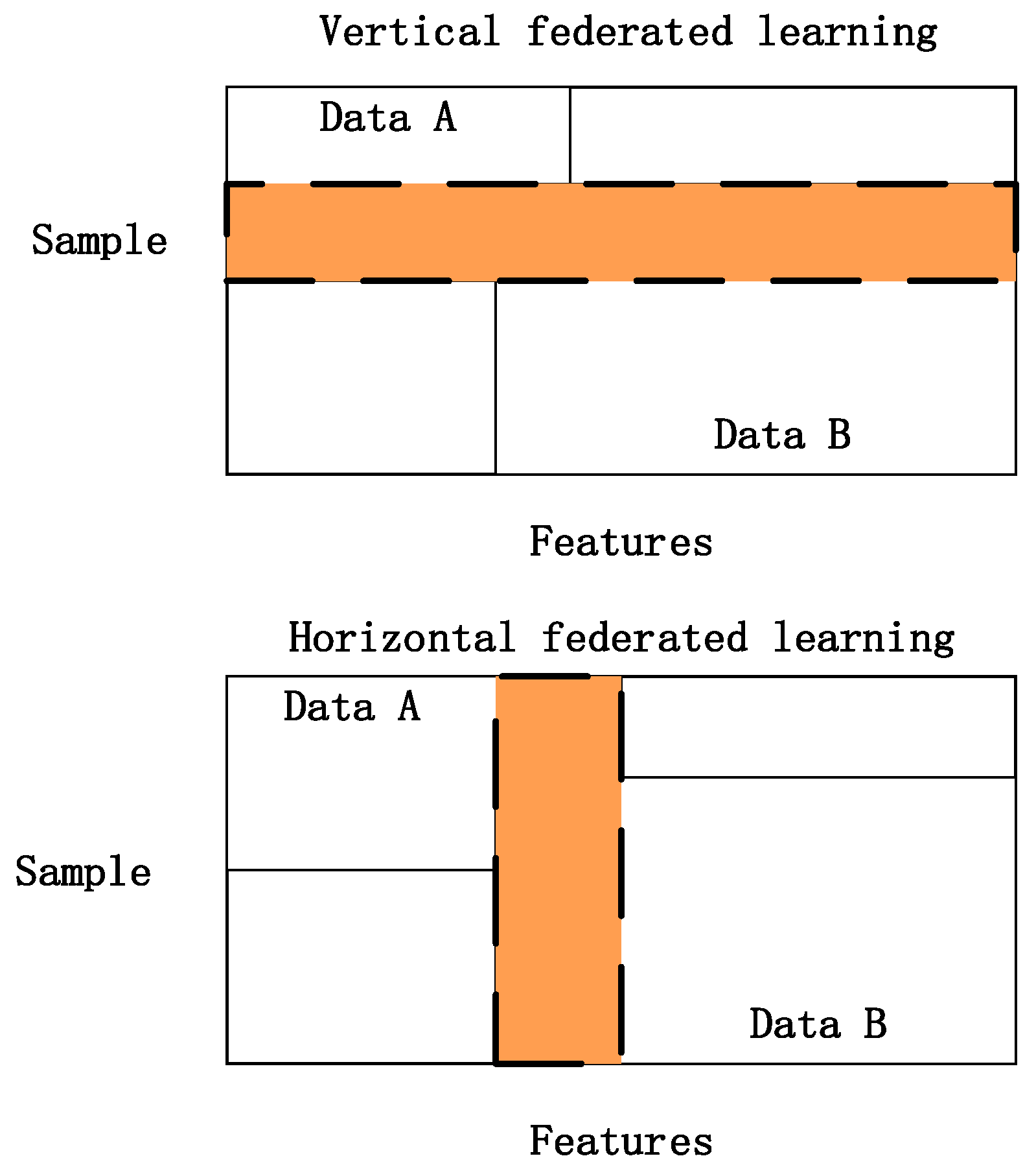
2.1. Transfer Learning and Federated Transfer Learning
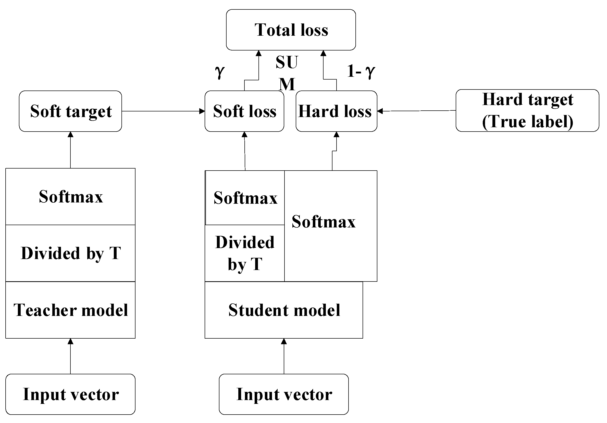
2.2. Knowledge Distillation
2.2.1. Single Teacher-Based Distillation
2.2.2. Multi-Teacher-Based Knowledge Distillation
3. Proposed Method
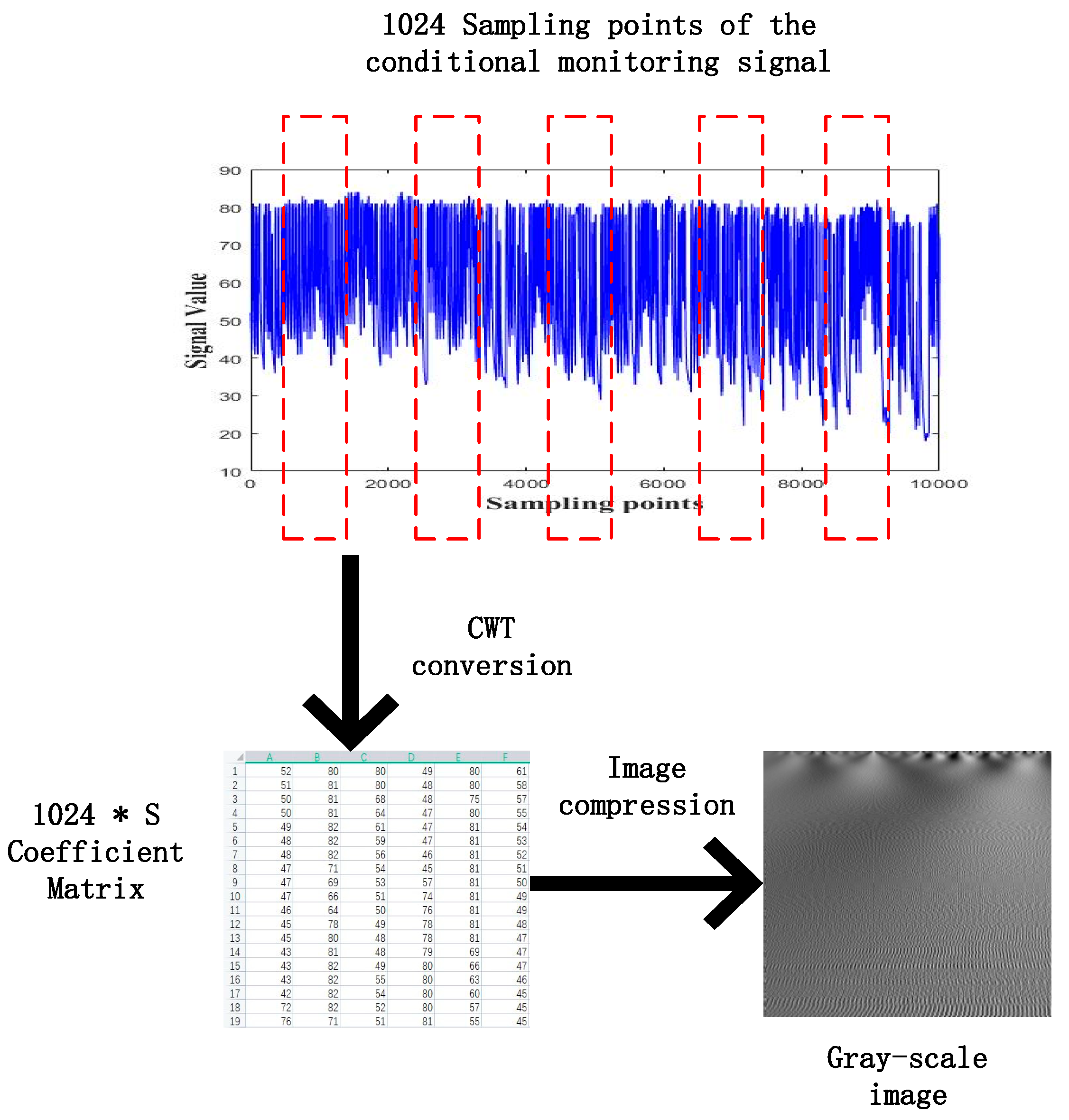
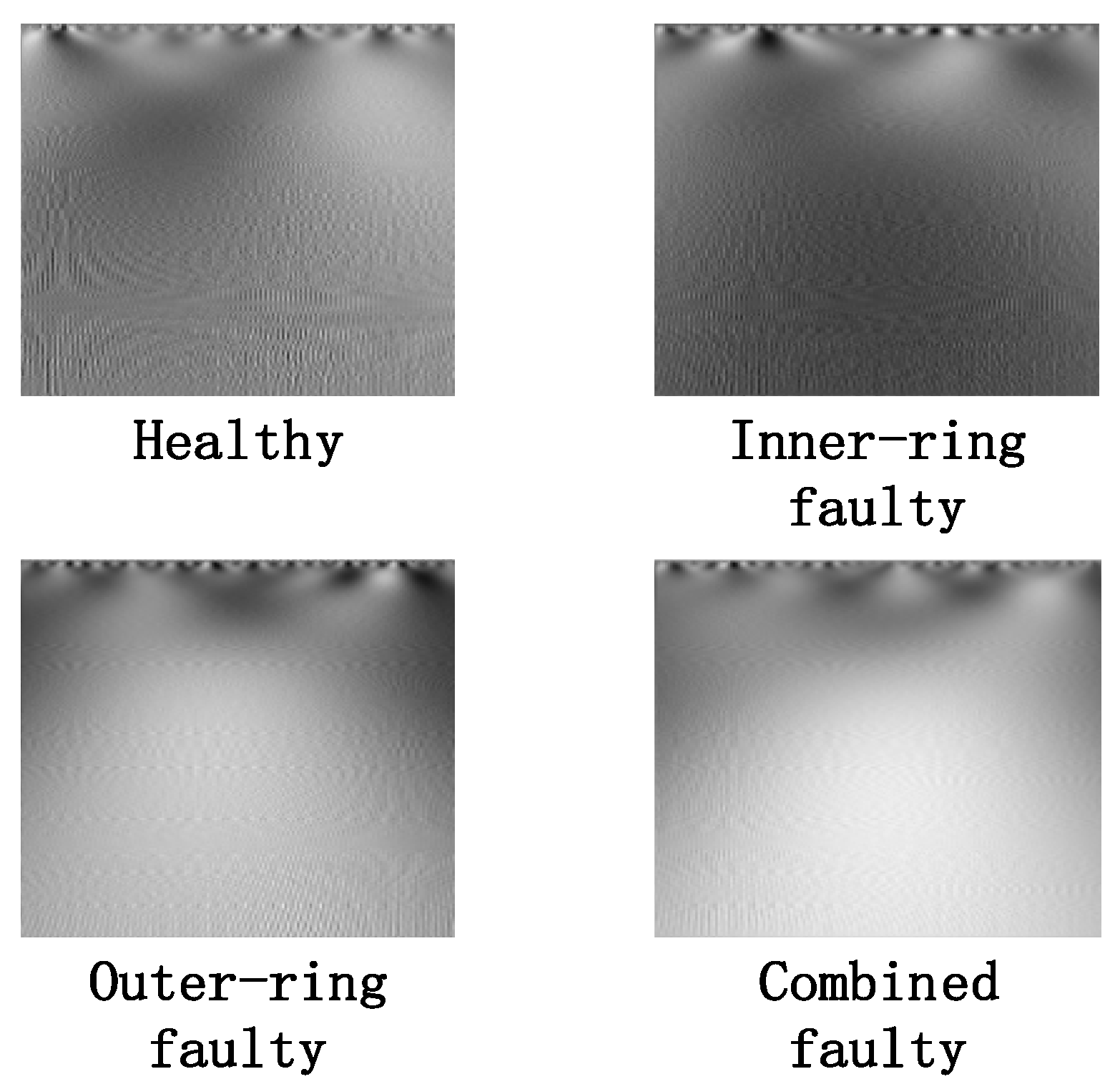
3.1. Data Preprocessing
3.2. Proposed FTLKD Frame Work
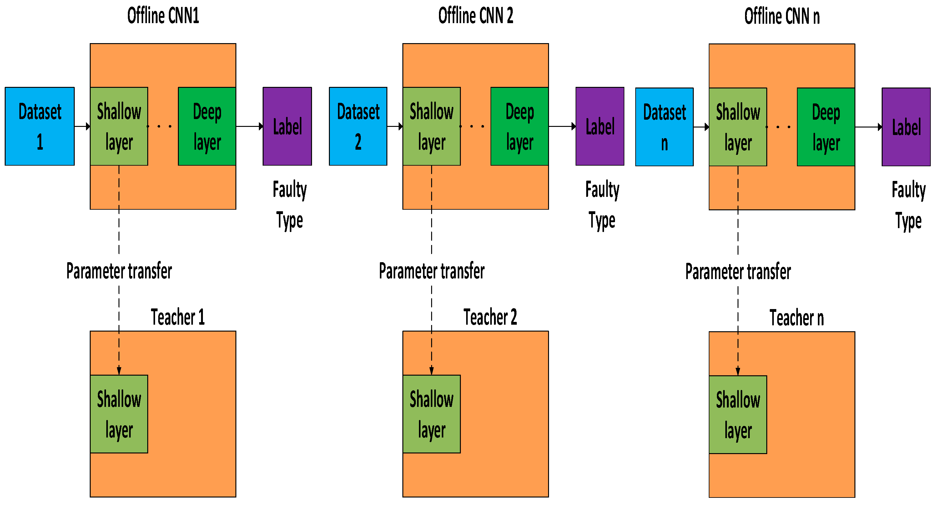
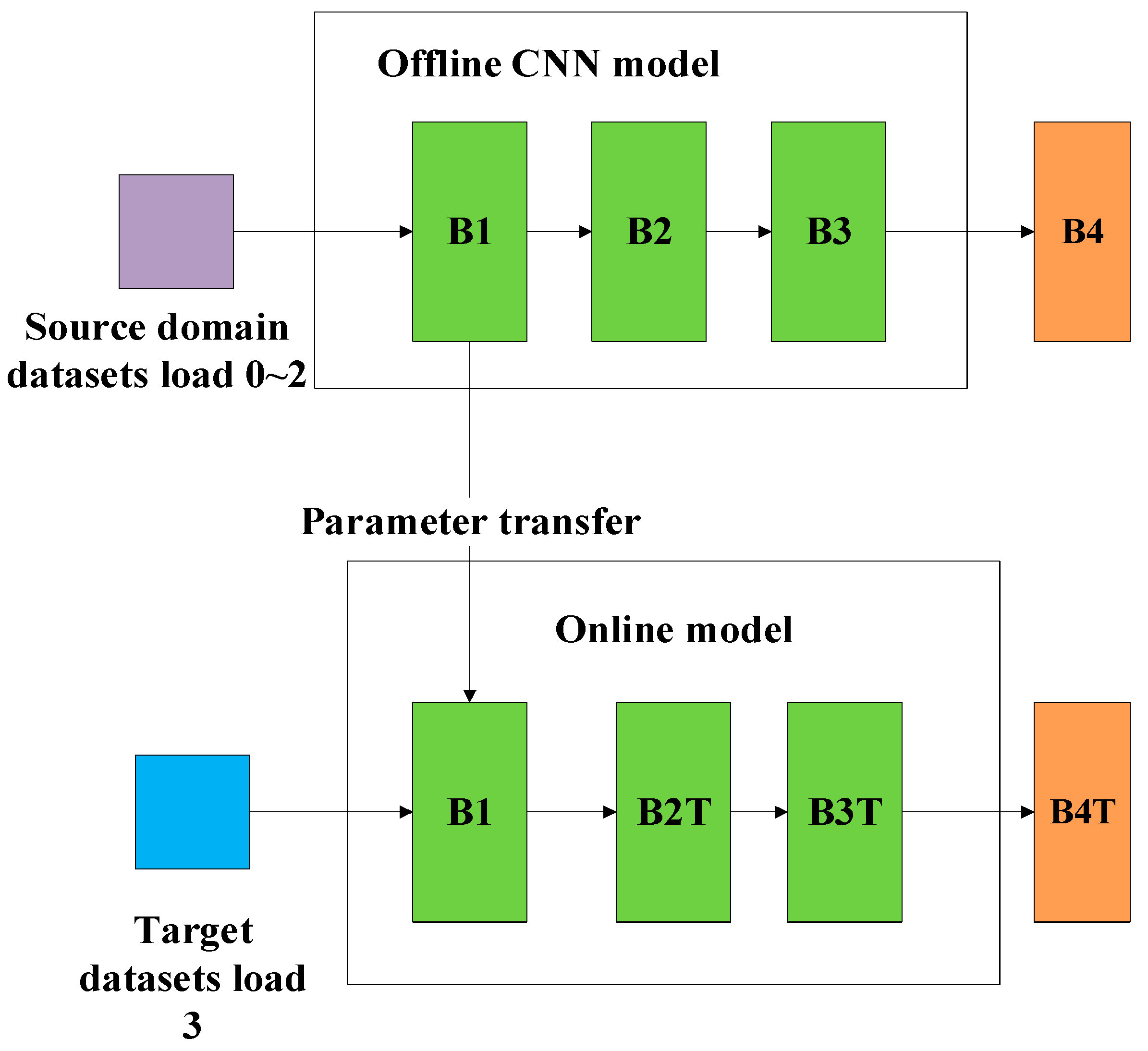
3.2.1. Multi Teachers Establishment Based on Federated Transfer Learning
3.2.2. Multi Sources Knowledge Transference Based on Knowledge Distillation
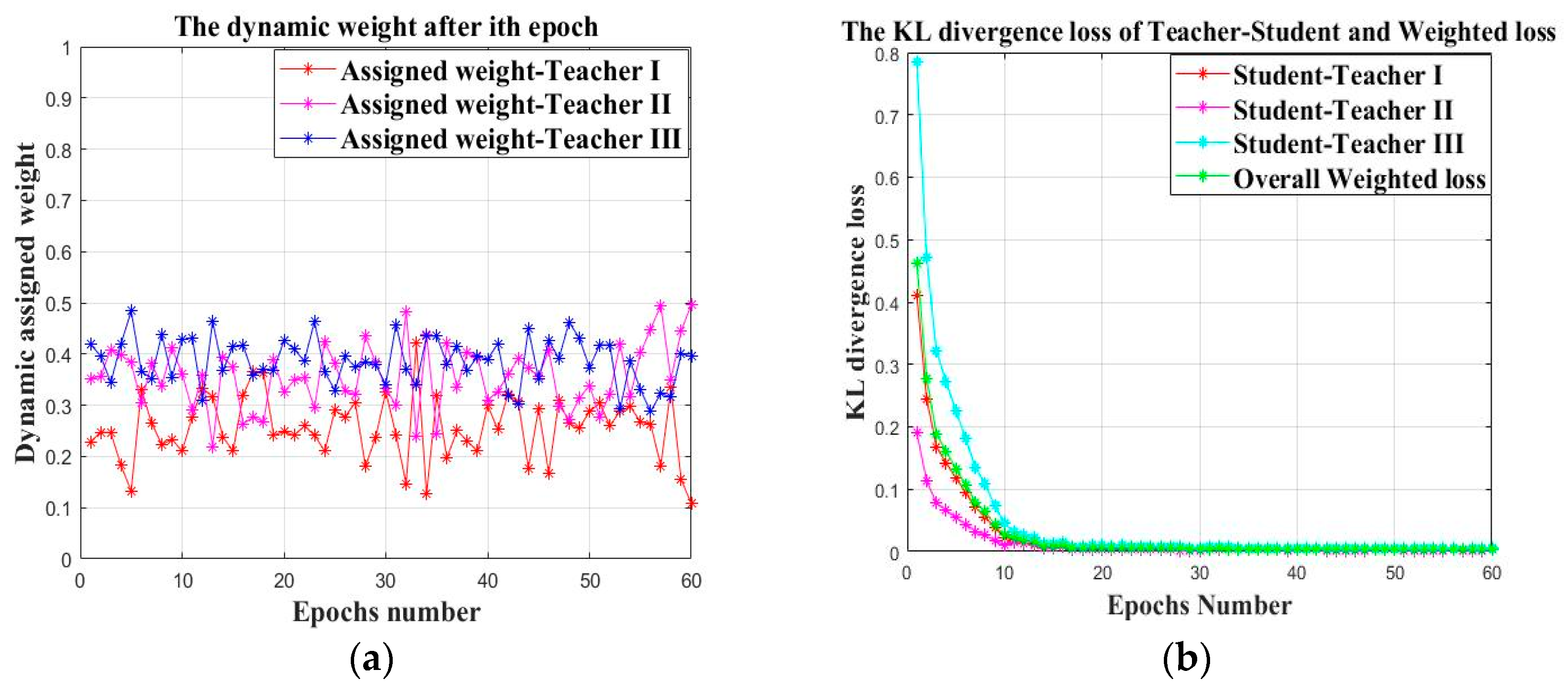
3.2.3. Teacher Balancing Based on KL Divergence
| Algorithm 1: General procedure of the proposed faulty prediction methodology |
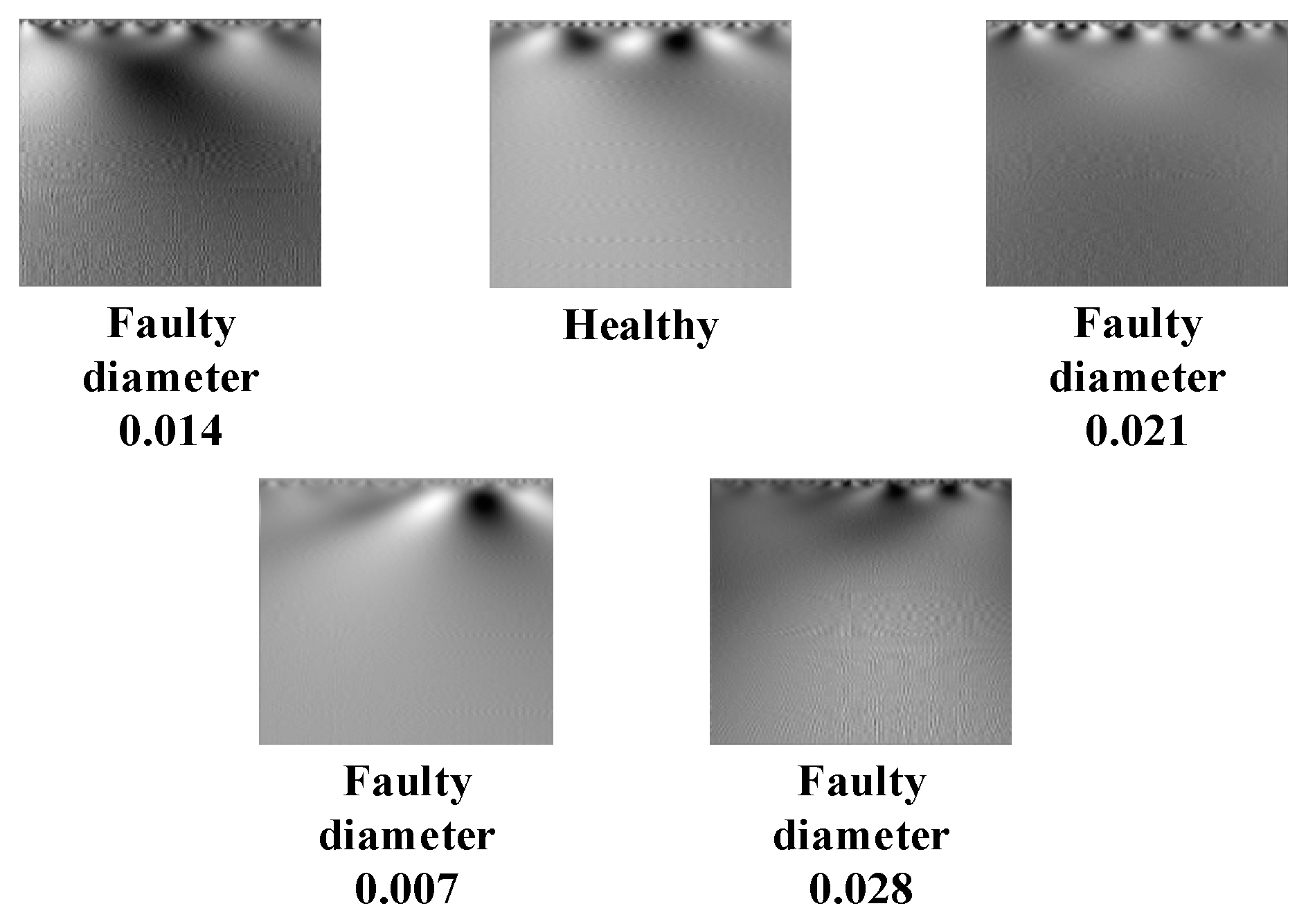
| Input: Given the source datasetsfor the offline establishment of the teacher models and the target datasetsfor the cooperative training of the teacher models and the student model. Output: The trained student model and the faulty prediction result. Step 1: Generate the training datasets and the testing datasets Obtain the two-dimensional gray scale images of the one-dimensional time series signal by using the “signal-to-image” conversion method based on the “Continuous Wavelet Transform” as shown in Figure 4. Step 2: Construct the teacher models by using the federated transfer learning 2.1: Randomly initializing several offline CNNs and pretraining these offline CNNs on the corresponding given source datasets . After these offline CNN models finish training on their own source datasets, their optimized weight “W” and bias ”b” can be obtained by solving the minimum of the loss metric using the Adam method. 2.2: Establishing the corresponding teacher model by transferring the shallow layers of the pretrained offline CNN to the standby teacher models as shown in Figure 5, while the parameters of the other layers are randomly initialized. Step 3: Multi-teacher-based knowledge distillation 3.1: Constructing the proposed teacher-student distillation framework as shown in Figure 6. 3.2: Fine-tuning the teacher models on the training set of the target datasets and calculating the KL divergence loss of the teacher model as shown in equation (6) 3.3: Dynamically update the assigned weight of teacher models during the distillation process based on the KL divergence loss of different teacher models, respectively, after each epoch as shown in equation (7). 3.4: Distilling the student model by calculating the weighted loss function between the teacher softened outputs and the student softened output as shown from equations (8) to (10). Step 4: Analysis of teacher models and the student model 4.1: Optimizing the student model through the cooperative training process by using the game strategy proposed in the literature [31,32] on the training set of the target datasets during step 3 and achieve the optimized student model. 4.2: Evaluating the testing accuracy of teacher models and the student model on the testing set of the target datasets . Step 5: Evaluate the proposed teacher-student distillation framework. Validate the performance of the obtained student model with a different teacher-student distillation framework and output the faulty prediction results. |
4. Case Studies and Experimental Result Discussion
4.1. Case Study I Bearing Faulty Prediction of the Electro-Mechanical Drive System
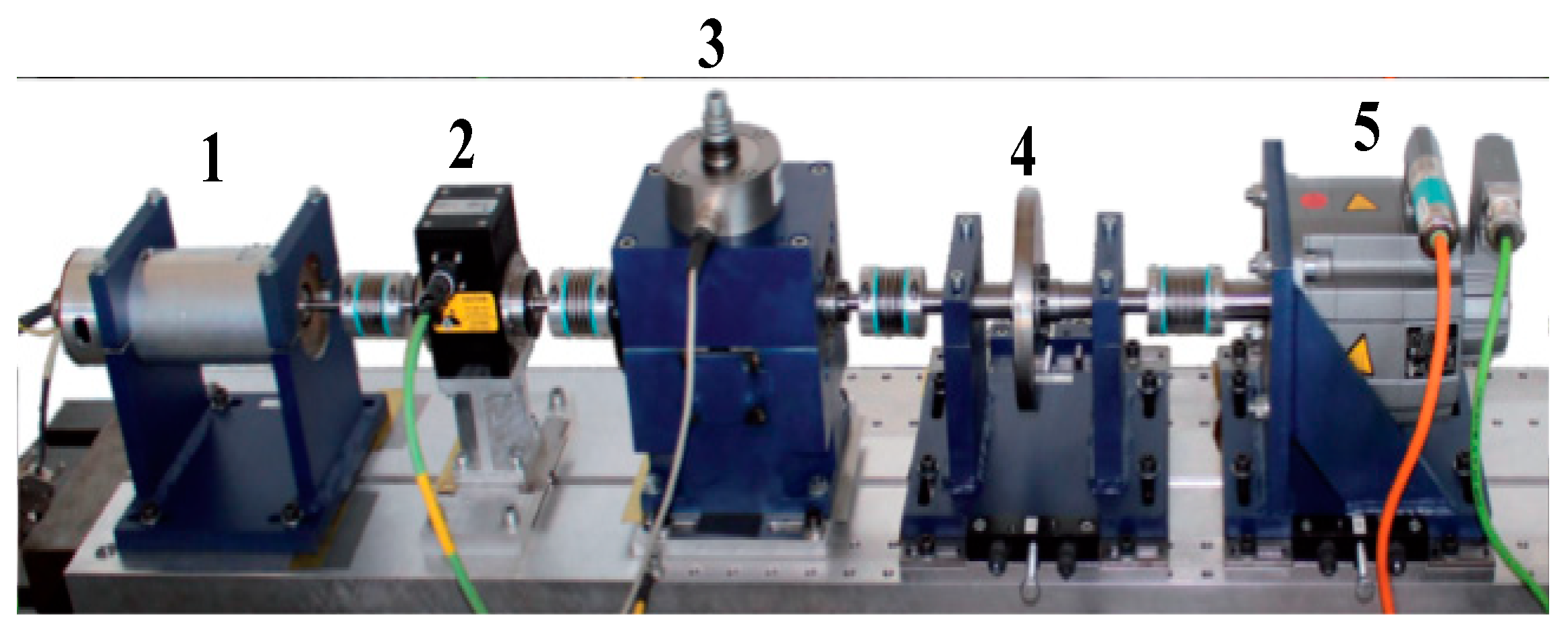
4.1.1. Data Description and Experimental Set Up
4.1.2. Data Preprocessing
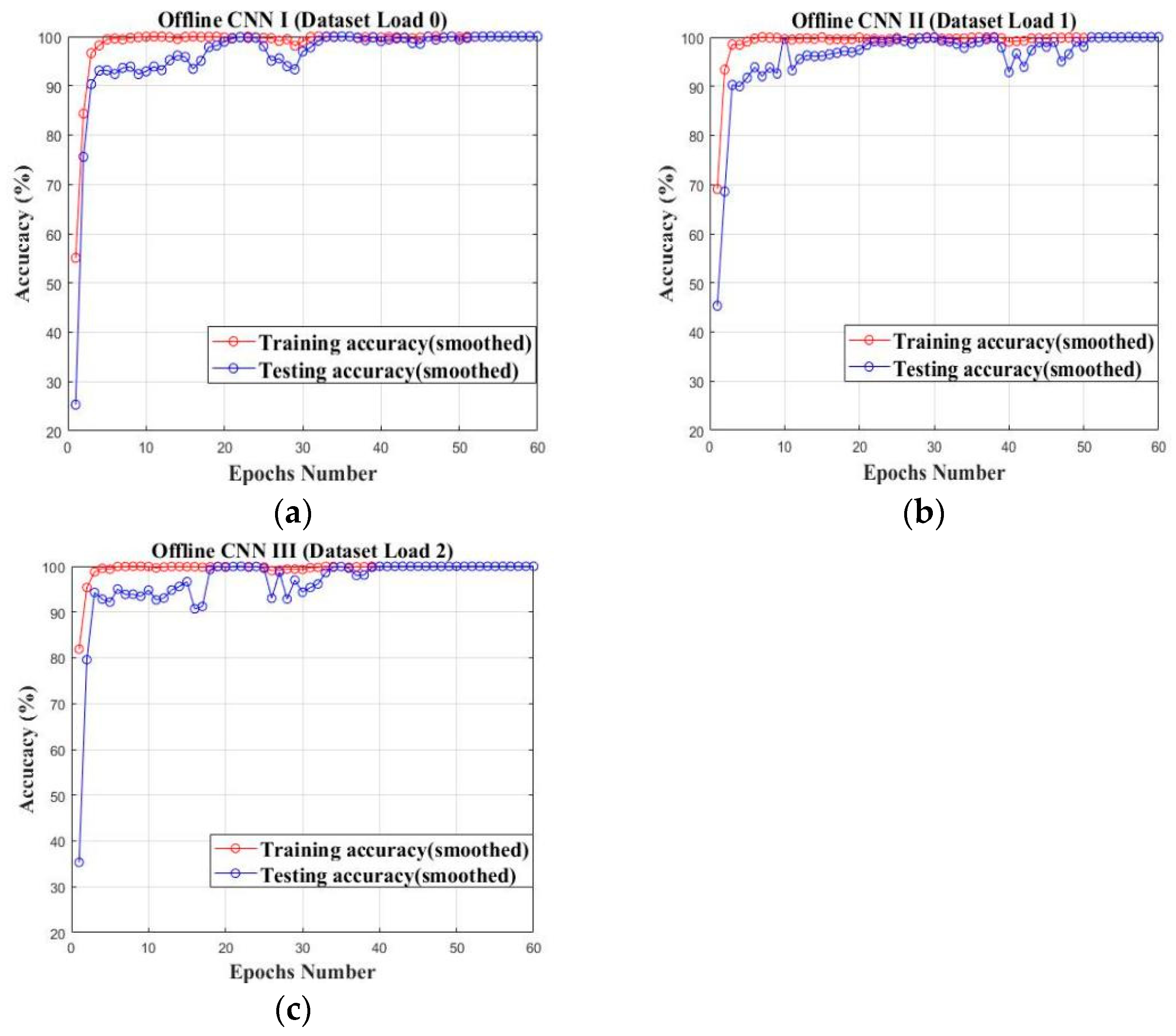
4.1.3. Offline CNN Models Set Up Based on Offline Training
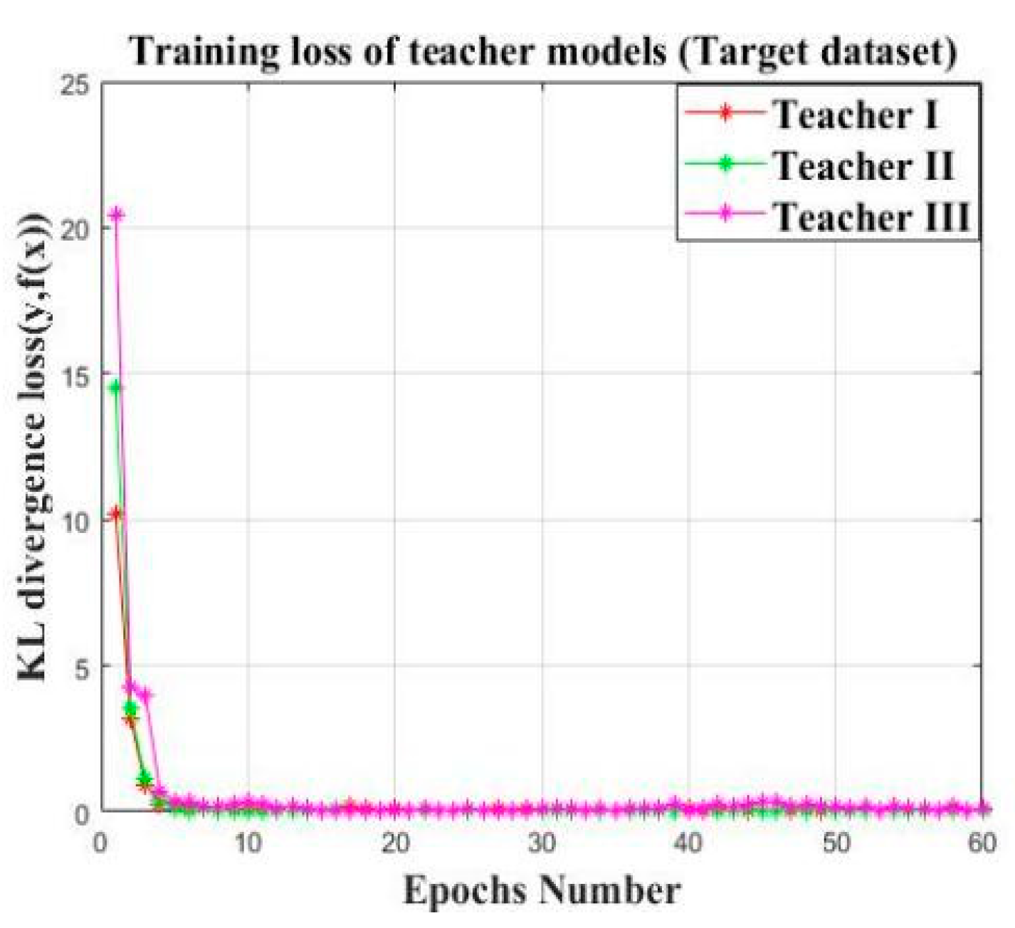
4.1.4. Teacher Establishment Based on Federated Transfer Learning
4.1.5. Knowledge Transference Based on Knowledge Distillation
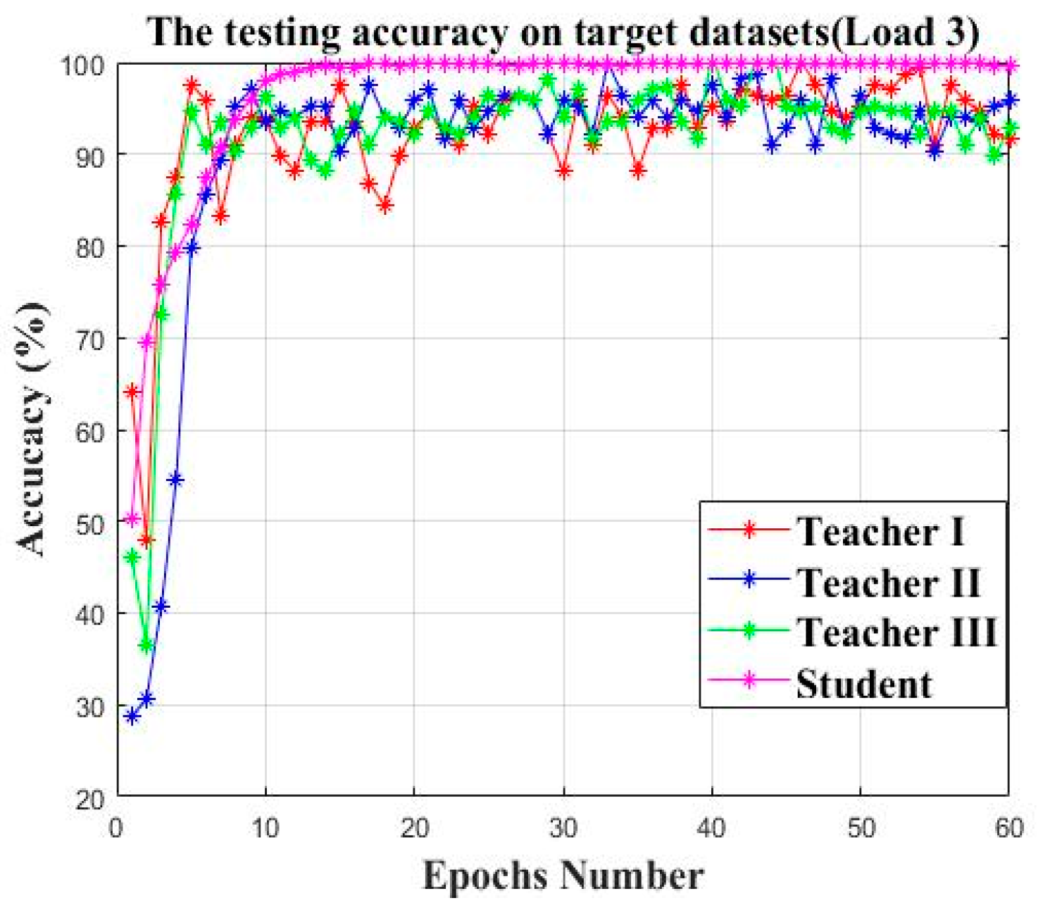
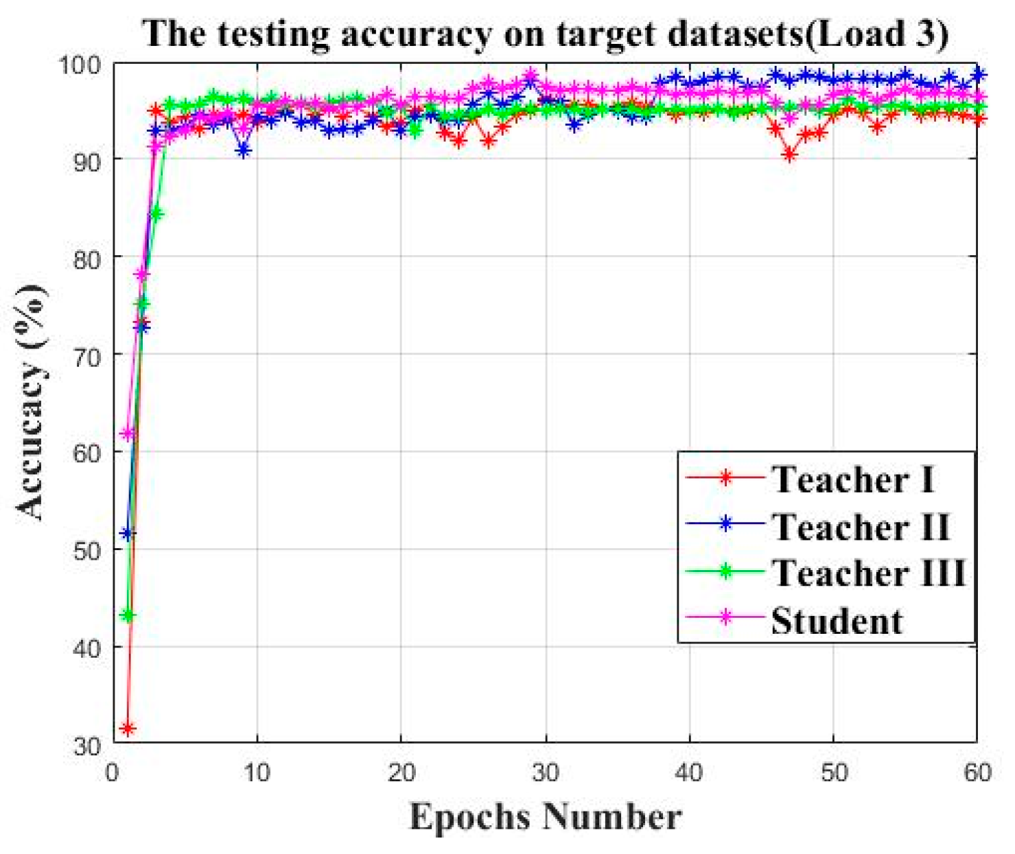
4.1.6. Model Evaluation
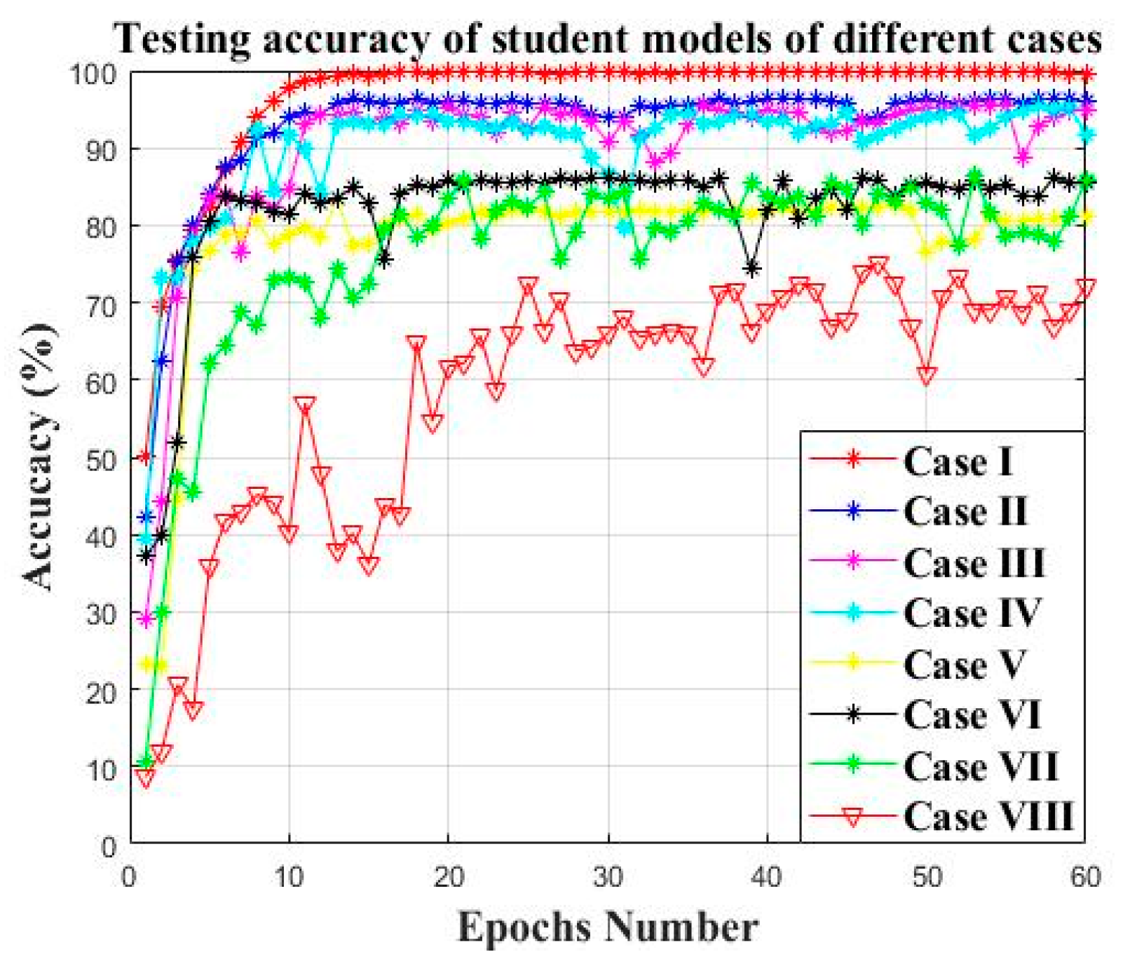
4.1.7. Comparison with Other Distillation Frameworks
4.1.8. Comparison with Other Machine Learning Models
4.2. Case Study II: Bearing Faulty Prediction for Reliance Electric Motor
4.2.1. Data Description and Experimental Set Up
4.2.2. Data Preprocessing
4.2.3. Private Models Establishment Based on Offline Private Training
4.2.4. Teacher Establishment Based on Federated Transfer Learning
4.2.5. Knowledge Transference Based on Knowledge Distillation
4.2.6. Model Evaluation
4.2.7. Comparison with Other Distillation Frameworks
4.2.8. Comparison with Other Machine Learning Models
5. Contribution and Future Work
5.1. Main Contribution of This Paper
- (1)
- The “signal to image” conversion method based on the continuous wavelet transform in the literature [5] is introduced to the data pre-processing of this paper which can well represent the information of machine health conditions contained in the raw signal.
- (2)
- Proposing a novel federated transfer learning framework (FTL) which contains prior knowledge from multiple different but related source domain areas. Several cumbersome models are pretrained on the datasets of multiple related areas, contributing different knowledge for the knowledge compensation of the transfer learning. The performance of the federated transfer learning model will not rely on a single source domain, enhancing the model’s generalization ability.
- (3)
- Proposing a novel multi-teacher-based knowledge distillation (KD) framework. The student model is guided by several teachers and the teacher models are dynamically weighted based on the real time KL divergence loss between the teacher output and the true label. The student model can obtain knowledge from different teachers with a lower parameter size which can be applicable for the edge computing-based deployment.
5.2. Future Work of This Paper
- (1)
- In this paper, the proposed federated transfer model is constructed based on the set up of multiple teacher models; however, it is laborious and costly to pretrain multiple teachers from different but related areas. Moreover, the weight assignment of the teacher models will become complicated with the increase in teacher models;
- (2)
- In this paper, the “Knowledge” learned by multiple teacher models from multiple related datasets are more likely to represent the basic features of multiple datasets. Further, the whole process of knowledge learning and knowledge transference is entirely based on the black-box theory, indicating that it is not able to be explained.
- (3)
- In this paper, the proposed bearing faulty prediction only offers the conditional prediction of the bearing status. However, it has not been extended to the determination of the maintenance strategy which might be more meaningful to the practical industry.
Author Contributions
Funding
Institutional Review Board Statement
Informed Consent Statement
Data Availability Statement
Conflicts of Interest
References
- Yaguo, L.; Naipeng, L.; Liang, G.; Ningbo, L.; Tao, Y.; Jing, L. Machinery health prognostics: A systematic review from data acquisition to RUL prediction. Mech. Syst. Signal Process. 2018, 104, 799–834. [Google Scholar]
- Peng, K.; Jiao, R.; Dong, J.; Yanting, P. A deep belief network based health indicator construction and remaining useful life prediction using improved particle filter. Neurocomputing 2019, 361, 19–28. [Google Scholar] [CrossRef]
- Shao, H.; Jiang, H.; Zhang, H.; Liang, T. Electric Locomotive Bearing Fault Diagnosis Using a Novel Convolutional Deep Belief Network. IEEE Trans. Ind. Electron. 2017, 65, 2727–2736. [Google Scholar] [CrossRef]
- Chen, Z.; Li, W. Multi-sensor Feature Fusion for Bearing Fault Diagnosis Using Sparse Autoencoder and Deep Belief Network. IEEE Trans. Instrum. Meas. 2017, 66, 1693–1702. [Google Scholar] [CrossRef]
- Xu, G.; Liu, M.; Jiang, Z.; Söffker, D.; Shen, W. Bearing Fault Diagnosis Method Based on Deep Convolutional Neural Network and Random Forest Ensemble Learning. Sensors 2019, 19, 1088. [Google Scholar] [CrossRef] [Green Version]
- Xiao, D.; Huang, Y.; Qin, C. Transfer learning with convolutional neural networks for small sample size problem in machinery fault diagnosis. Arch. Proc. Inst. Mech. Eng. Part C J. Mech. Eng. Sci. 2019, 233, 5131–5143. [Google Scholar] [CrossRef]
- Cao, P.; Zhang, S.; Tang, J. Pre-Processing-Free Gear Fault Diagnosis Using Small Datasets with Deep Convolutional Neural Network-Based Transfer Learning. IEEE Access 2017, 6, 26241–26253. [Google Scholar] [CrossRef]
- Han, T.; Liu, C.; Yang, W.; Jiang, D. Deep Transfer Network with Joint Distribution Adaptation: A New Intelligent Fault Diagnosis Framework for Industry Application. ISA Trans. 2019, 97, 269–281. [Google Scholar] [CrossRef] [Green Version]
- Wen, L.; Gao, L.; Li, X. A New Deep Transfer Learning Based on Sparse Auto-Encoder for Fault Diagnosis. IEEE Trans. Syst. Man Cybern. Syst. 2019, 49, 136–144. [Google Scholar] [CrossRef]
- Wang, C.; Mahadevan, S. Heterogeneous Domain Adaptation Using Manifold Alignment. In Proceedings of the International Joint Conference on IJCAI, DBLP, Barcelona, Spain, 16–22 July 2011. [Google Scholar]
- Liu, Y.; Kang, Y.; Xing, C.; Chen, T.; Yang, Q. A Secure Federated Transfer Learning Framework. Intell. Syst. IEEE 2020, 35, 70–82. [Google Scholar] [CrossRef]
- Huang, T.; Lin, W.; Wu, W.; He, L.; Li, K.; Zomaya, A.Y. An Efficiency-boosting Client Selection Scheme for Federated Learning with Fairness Guarantee. IEEE Trans. Parallel Distrib. Syst. 2020, 32, 1552–1564. [Google Scholar] [CrossRef]
- Szepesvári, C. Synthesis Lectures on Artificial Intelligence and Machine Learning; Morgan & Claypool: San Rafael, CA, USA, 2019. [Google Scholar]
- Yang, Q. Federated learning: The last on kilometer of artificial intelligence. CAAI Trans. Intell. Syst. 2020, 15, 183–186. [Google Scholar]
- McMahan, H.B.; Moore, E.; Ramage, D.; Arcas, B.A. Federated Learning of Deep Networks using Model Averaging. arXiv 2016, arXiv:1602.05629. [Google Scholar]
- Ju, C.; Gao, D.; Mane, R.; Tan, B.; Liu, Y.; Guan, C. Federated Transfer Learning for EEG Signal Classification. In Proceedings of the 2020 42nd Annual International Conference of the IEEE Engineering in Medicine & Biology Society (EMBC), Montreal, QC, Canada, 20–24 July 2020. [Google Scholar]
- Wang, A.; Zhang, Y.; Yan, Y. Heterogeneous Defect Prediction Based on Federated Transfer Learning via Knowledge Distillation. IEEE Access 2021, 9, 29530–29540. [Google Scholar] [CrossRef]
- Sharma, S.; Xing, C.; Liu, Y.; Kang, T. Secure and Efficient Federated Transfer Learning. In Proceedings of the 2019 IEEE International Conference on Big Data (Big Data), Los Angeles, CA, USA, 9–12 December 2019. [Google Scholar]
- Hinton, G.; Dean, J.; Vinyals, O. Distilling the Knowledge in a Neural Network. arXiv 2014, arXiv:1503.02531. [Google Scholar]
- Alkhulaifi, A.; Alsahli, F.; Ahmad, I. Knowledge distillation in deep learning and its applications. PeerJ Comput. Sci. 2021, 7, e474. [Google Scholar] [CrossRef]
- Romero, A.; Ballas, N.; Kahou, S.E.; Chassang, A.; Bengio, Y. FitNets: Hints for Thin Deep Nets. arXiv 2015, arXiv:1412.6550. [Google Scholar]
- Markov, K.; Matsui, T. Robust Speech Recognition Using Generalized Distillation Framework. Interspeech 2016, 2364–2368. [Google Scholar] [CrossRef]
- Chebotar, Y.; Waters, A. Distilling Knowledge from Ensembles of Neural Networks for Speech Recognition. Interspeech 2016, 3439–3443. [Google Scholar] [CrossRef] [Green Version]
- Yuan, M.; Peng, Y. CKD: Cross-Task Knowledge Distillation for Text-to-Image Synthesis. IEEE Trans. Multimed. 2020, 22, 1955–1968. [Google Scholar] [CrossRef]
- Huang, S.J.; Hsieh, C.T. High-impedance fault detection utilizing a morlet wavelet transform approach. IEEE Trans. Power Deliv. 1999, 14, 1401–1410. [Google Scholar] [CrossRef]
- Lin, J.; Liangsheng, Q.U. Feature Extraction Based on Morlet Wavelet and Its Application for Mechanical Fault Diagnosis. J. Sound Vib. 2000, 234, 135–148. [Google Scholar] [CrossRef]
- Sun, J.; Yan, C.; Wen, J. Intelligent Bearing Fault Diagnosis Method Combining Compressed Data Acquisition and Deep Learning. IEEE Trans. Instrum. Meas. 2017, 67, 185–195. [Google Scholar] [CrossRef]
- Long, W.; Xinyu, L.; Gao, L.; Zhang, Y. A New Convolutional Neural Network-Based Data-Driven Fault Diagnosis Method. IEEE Trans. Ind. Electron. 2017, 65, 5990–5998. [Google Scholar]
- Min, X.; Teng, L.; Lin, X.; Liu, L.; de Silva, C.W. Fault Diagnosis for Rotating Machinery Using Multiple Sensors and Convolutional Neural Networks. IEEE/ASME Trans. Mechatron. 2017, 23, 101–110. [Google Scholar]
- Ding, X.; He, Q. Energy-Fluctuated Multi-scale Feature Learning With Deep ConvNet for Intelligent Spindle Bearing Fault Diagnosis. IEEE Trans. Instrum. Meas. 2017, 66, 1926–1935. [Google Scholar] [CrossRef]
- Wong, K. Bridging game theory and the knapsack problem: A theoretical formulation. J. Eng. Math. 2015, 91, 177–192. [Google Scholar] [CrossRef]
- Wong, K. A Geometrical Perspective for the Bargaining Problem. PLoS ONE 2010, 5, e10331. [Google Scholar] [CrossRef] [Green Version]
- Lessmeier, C.; Kimotho, J.K.; Zimmer, D.; Sextro, W. Condition Monitoring of Bearing Damage in Electromechanical Drive Systems by Using Motor Current Signals of Electric Motors: A Benchmark Data Set for Data-Driven Classification. In Proceedings of the European Conference of the PHM Society, Bilbao, Spain, 5–8 July 2016; Volume 3. [Google Scholar] [CrossRef]
- Loparo, K. Case Western Reserve University Bearing Data Centre Website. 2012. Available online: https://engineering.case.edu/bearingdatacenter/12k-drive-end-bearing-fault-data (accessed on 12 December 2018).


| Loads | Rotational Speed [Rpm] | Load Torque [Nm] | Radial Force [N] | Name of Setting |
|---|---|---|---|---|
| 0 | 1500 | 0.7 | 1000 | N15_M07_F10 |
| 1 | 900 | 0.7 | 1000 | N09_M07_F10 |
| 2 | 1500 | 0.1 | 1000 | N15_M01_F10 |
| 3 | 1500 | 0.7 | 400 | N15_M07_F04 |
| Motor Load (HP) | Data Sample Quantity (Training/Testing) | Datasets Assignment |
|---|---|---|
| Load 0 | 1000/1000 | Datasets for Teacher I |
| Load 1 | 1000/1000 | Datasets for Teacher II |
| Load 2 | 1000/1000 | Datasets for Teacher III |
| Load 3 | 100/100 | Target datasets for Teachers & Student |
| Block | Layer Number | Layer Type | Kernel Size | Kernel Number | Stride | Padding |
|---|---|---|---|---|---|---|
| B1 | 1 | Conv | 32 | 1 | Same | |
| 2 | BN | - | - | - | - | |
| 3 | Conv | 32 | 1 | Same | ||
| 4 | BN | - | - | - | - | |
| 5 | Conv | 32 | 2 | Same | ||
| 6 | BN | - | - | - | - | |
| B2 | 7 | Conv | 64 | 1 | Same | |
| 8 | BN | - | - | - | - | |
| 9 | Conv | 64 | 1 | Same | ||
| 10 | BN | - | - | - | - | |
| 11 | Conv | 64 | 2 | Same | ||
| 12 | BN | - | - | - | - | |
| B3 | 13 | Conv | 128 | 1 | Same | |
| 14 | BN | - | - | - | - | |
| 15 | Conv | 128 | 1 | Same | ||
| 16 | BN | - | - | - | - | |
| 17 | Conv | 128 | 2 | Same | ||
| 18 | BN | - | - | - | - | |
| B4 | 19 | FC | 1000 | - | - | - |
| 20 | Dense | 32 | - | - | - | |
| 21 | Softmax | 4 | - | - | - |
| Block | Layer Number | Layer Type | Kernel Size | Kernel Number | Stride | Padding |
|---|---|---|---|---|---|---|
| S1 | 1 | Conv | 32 | 1 | Same | |
| 2 | BN | - | - | - | - | |
| 3 | Conv | 32 | 1 | Same | ||
| 4 | BN | - | - | - | - | |
| 5 | Conv | 32 | 2 | Same | ||
| 6 | BN | - | - | - | - | |
| S2 | 7 | FC | 1000 | - | - | - |
| 8 | Dense | 32 | - | - | - | |
| 9 | Softmax | 4 | - | - | - |
| Model | Average Accuracy (%) | Parameter Number | Average KL Divergence Loss |
|---|---|---|---|
| Teacher I | 94.58% | 4,677,924 | 3.59 |
| Teacher II | 98.13% | 4,677,924 | 0.77 |
| Teacher III | 95.44% | 4,677,924 | 0.47 |
| Student | 96.69% | 1,142,764 | 0.02 |
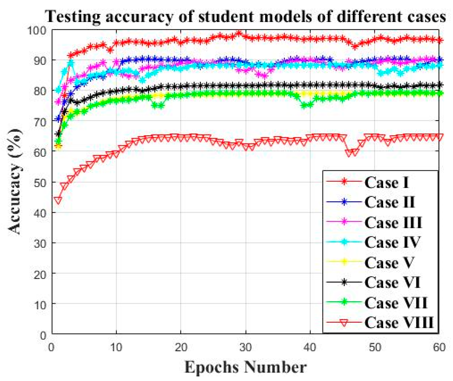
| Method | Teacher Number | Datasets I (Load 0) | Datasets II (Load 1) | Datasets III (Load 2) |
|---|---|---|---|---|
| Case I | 3 | Teacher 1 | Teacher 2 | Teacher 3 |
| Case II | 2 | Teacher 1 | Teacher 2 | |
| Case III | 2 | Teacher 2 | Teacher 3 | |
| Case IV | 2 | Teacher 1 | Teacher 3 | |
| Case V | 1 | Teacher 1 | ||
| Case VI | 1 | Teacher 2 | ||
| Case VII | 1 | Teacher 3 | ||
| Case VIII | 0 | No teacher | ||
| Method | Average Testing Accuracy | Average KL Divergence Loss |
|---|---|---|
| Case I | 96.69% | 0.02 |
| Case II | 88.07% | 0.048 |
| Case III | 87.65% | 0.051 |
| Case IV | 87.05% | 0.093 |
| Case V | 77.73% | 0.339 |
| Case VI | 80.47% | 0.675 |
| Case VII | 79.35% | 0.474 |
| Case VIII | 62.19% | 10.115 |
| Method | Prior Knowledge | Average Testing Accuracy | Average Testing Loss (KL Divergence Loss) |
|---|---|---|---|
| Student model | Guided by three teachers | 96.69% | 0.02 |
| Teacher I | Pre-trained on Datasets I | 94.58% | 3.59 |
| Teacher II | Pre-trained on Datasets II | 98.13% | 0.77 |
| Teacher III | Pre-trained on Datasets III | 95.44% | 0.49 |
| DAE | No prior knowledge | 91.31% | 14.27 |
| BPNN | No prior knowledge | 81.31% | 10.66 |
| DBN | No prior knowledge | 89.17% | 15.31 |
| SVM | No prior knowledge | 82.62% | 15.94 |
| CNN (Structure of teacher model) | No prior knowledge | 87.66% | 15.12 |
| Rotating Speed (rpm) | Data Sample Quantity (Training/Testing) | Datasets Assignment |
|---|---|---|
| Load 0 (1730 rpm) | 1000/1000 | Datasets for teacher I |
| Load 1 (1750 rpm) | 1000/1000 | Datasets for teacher II |
| Load 2 (1772 rpm) | 1000/1000 | Datasets for teacher III |
| Load 3 (1797 rpm) | 100/100 | Datasets for teacher IV |
| Model | Average Accuracy (%) | Parameter Size | Average KL Divergence Loss |
|---|---|---|---|
| Teacher I | 95.12% | 4,677,924 | 2.63 |
| Teacher II | 94.63% | 4,677,924 | 3.59 |
| Teacher III | 94.81% | 4,677,924 | 5.73 |
| Student | 99.83% | 1,142,764 | 0.076 |
| Method | Average Accuracy | Average KL Divergence Loss |
|---|---|---|
| Case I | 99.83% | 0.076 |
| Case II | 93.04% | 0.094 |
| Case III | 90.04% | 0.171 |
| Case IV | 91.07% | 0.114 |
| Case V | 78.08% | 1.154 |
| Case VI | 82.01% | 1.782 |
| Case VII | 76.27% | 2.796 |
| Case VIII | 58.74% | 12.919 |
| Method | Prior Knowledge | Average Testing Accuracy | Average Testing Loss |
|---|---|---|---|
| Student model | Guided by three teachers | 99.83% | 0.076 |
| Teacher I | Pre-trained on load 0 | 95.12% | 2.63 |
| Teacher II | Pre-trained on load 1 | 94.63% | 3.59 |
| Teacher III | Pre-trained on load 2 | 94.81% | 5.73 |
| DAE | No prior knowledge | 78.45% | 10.38 |
| BPNN | No prior knowledge | 86.58% | 11.56 |
| DBN | No prior knowledge | 87.55% | 9.92 |
| SVM | No prior knowledge | 81.45% | 6.21 |
| CNN (structure of teacher model) | No prior knowledge | 90.45% | 7.18 |
Publisher’s Note: MDPI stays neutral with regard to jurisdictional claims in published maps and institutional affiliations. |
© 2022 by the authors. Licensee MDPI, Basel, Switzerland. This article is an open access article distributed under the terms and conditions of the Creative Commons Attribution (CC BY) license (https://creativecommons.org/licenses/by/4.0/).
Share and Cite
Zhou, Y.; Wang, J.; Wang, Z. Bearing Faulty Prediction Method Based on Federated Transfer Learning and Knowledge Distillation. Machines 2022, 10, 376. https://doi.org/10.3390/machines10050376
Zhou Y, Wang J, Wang Z. Bearing Faulty Prediction Method Based on Federated Transfer Learning and Knowledge Distillation. Machines. 2022; 10(5):376. https://doi.org/10.3390/machines10050376
Chicago/Turabian StyleZhou, Yiqing, Jian Wang, and Zeru Wang. 2022. "Bearing Faulty Prediction Method Based on Federated Transfer Learning and Knowledge Distillation" Machines 10, no. 5: 376. https://doi.org/10.3390/machines10050376
APA StyleZhou, Y., Wang, J., & Wang, Z. (2022). Bearing Faulty Prediction Method Based on Federated Transfer Learning and Knowledge Distillation. Machines, 10(5), 376. https://doi.org/10.3390/machines10050376