Bearing Faulty Prediction Method Based on Federated Transfer Learning and Knowledge Distillation

Abstract

In this paper, a novel bearing faulty prediction method based on federated transfer learning and knowledge distillation is proposed with three stages: (1) a “signal to image” conversion method based on the continuous wavelet transform is used as the data pre-processing method to satisfy the input characteristic of the proposed faulty prediction model; (2) a novel multi-source based federated transfer learning method is introduced to acquire knowledge from multiple different but related areas, enhancing the generalization ability of the proposed model; and (3) a novel multi-teacher-based knowledge distillation is introduced as the knowledge transference way to transfer multi-source knowledge with dynamic importance weighting, releasing the target data requirement and the target model parameter size, which makes it possible for the edge-computing based deployment. The effectiveness of the proposed bearing faulty prediction approach is evaluated on two case studies of two public datasets offered by the Case Western Reserve University and the Paderborn University, respectively. The evaluation result shows that the proposed approach outperforms other state-of-the-art faulty prediction approaches in terms of higher accuracy and lower parameter size with limited labeled target data.

1. Introduction

Intelligent faulty diagnosis is significantly important in the modern manufacturing industry as it can greatly reduce the machine maintenance cost and prevent catastrophic failure in the early stages of production. The current faulty prediction approaches can be divided into three categories: model based, knowledge based and data-driven based approaches [1]. With the development of the modern computing ability and storage capacity, the data-driven based machine faulty prediction approach has been the most used one. This is entirely based on the acquired historical operating datasets [2].

Deep learning, as a branch of the data-driven approach, has achieved compromising application prospects in the contemporary industrial system due to its powerful ability to automatically distinguish the representative and discriminative features from the raw signal data. Therefore, the deep learning-based faulty prediction method has become a key research point in both academia and industry. The current deep learning models, including the DBN (deep belief network), DAE (deep auto-encoder), RNN (recurrent neural network) and CNN (convolution neural network) have already achieved great success in the machine faulty prediction area. In order to further promote the machine faulty prediction accuracy in the application of the modern complex industry, some researchers have designed different variants and combinations of the deep learning models. Shao et al. [3] combined the CNN with DBN for capturing both the two-dimensional structure and the periodic characteristics of the input data. Chen et al. [4] combined the sparse auto-encoder (SAE) with the deep belief network where the SAE is used for the multi-sensor feature fusion and the DBN is used for the machine faulty prediction. In order to enhance the generalization ability of the prediction model, Xu et al. [5] proposed the LeNet-5 CNN based multi-scale feature extraction network where features learned from the multiple layers of CNN are extracted jointly for the bearing fault prediction. Although the deep learning-based faulty prediction model has achieved practical industrial use, two issues remain:

(1)

The training process of the traditional deep learning model requires large amounts of labeled data; however, in the practical industry, it is extremely costly to acquire labeled data, especially the labeled data representing the machine faulty condition which is usually not well preserved.

(2)

Since the traditional deep learning model is usually trained on large amounts of historical datasets, the model training process is usually time consuming due to its large training data volumes. How to accelerate the training process of the faulty prediction model remains a challenge.

In order to release the problem of insufficient labeled data and training time consumption, the deep learning approach based on transfer learning has been studied in recent literature. Transfer learning aims at transferring the knowledge learned from the related source domain to the target domain which can relax the requirement of the labeled training data and reduce the training time. Xiao et al. [6] proposed a TrAdaBoost based transfer learning framework with convolution neural networks for solving the small sample problem in machinery fault diagnosis. CAO et al. [7] proposed a deep convolution-based transfer learning for the gear faulty diagnosis with very limited training datasets. Han et al. [8] proposed a deep transfer neural network with joint distribution adaptation (JDA) for the intelligent faulty prediction. The proposed approach takes advantage of a pre-trained network from the source domain and the model is transferred with unlabeled data to the target domain by using the JDA, solving the problem of insufficient labeled data in practical industry. WEN et al. [9] proposed novel deep transfer learning (DTL) where the three-layer sparse auto-encoder is designed for the feature extraction of the raw data and the maximum mean discrepancy term is used to minimize the discrepancy penalty between the features from the source domain and the target domain. Despite the deep learning approaches based on transfer learning proving to be effective in releasing the data requirement and speeding up the training process of the traditional deep learning models, it is still questionable whether it is the most appropriate way to directly transfer the features or parameters from a single source domain model to the target domain model for the practical faulty prediction problem. Two points need to be further considered:

(1)

The performance of the traditional transfer learning model relies on the quality of the source data and the degree of similarity between the source domain and the target domain which poses limitations on the generalization ability of the transfer learning model. How to construct a generalized transfer learning framework that is applicable to different transfer learning tasks remains a great challenge.

(2)

With the increase in the transferred features and parameters from the original model which contains “knowledge” from different but related source domains, the parameter scale of the transfer learning model can be very large, causing difficulties for the model field deployment. How to release the parameter size of the transfer learning model remains a topic of consideration.

In order to release the single source domain limitation and the model parameter scale, a novel hybrid-bearing faulty prediction model based on the federated transfer learning and knowledge distillation (FTLKD) is proposed in this paper. Dealing with the above two listed issues, the contribution of this paper is listed as follows:

(1)

Dealing with the first issue listed above, several cumbersome models are set up through offline training on multiple related source domain datasets. Thus, containing prior knowledge of different source domain datasets;

(2)

Dealing with the second issue listed above, the cumbersome models pretrained on multiple different but related datasets are used as teacher models during the joint training process with the student model on the target datasets. This is also called knowledge distillation. The established teacher models can promote the training efficiency of the shallow structured student model while maintaining its small parameter size by using the knowledge distillation. The assigned weights of the teacher models are dynamically changed during the joint training process based on the real time KL-divergence loss between the corresponding teacher output and the true label.

The rest of this paper is organized as follows: Section 2 briefly reviews the related research background including the transfer learning, the federated transfer learning and the knowledge distillation; Section 3 presents the framework and specific technical detail of the proposed federated transfer learning and knowledge distillation based faulty prediction approach; Section 4 describes the case study and simulation result of the proposed approach. Finally, the main contribution and future work is proposed in Section 5.

2. Related Work

2.1. Transfer Learning and Federated Transfer Learning

The transfer learning aims at building an effective prediction model for an application with a limited quantity of labeled datasets in a target domain by leveraging rich labels from a different but related source domain, as shown in Figure 1. Provided that a learning task ${\mathrm{T}}_{\mathrm{s}}$is in the source domain ${\mathrm{D}}_{\mathrm{s}}$ and a prediction task ${\mathrm{T}}_{\mathrm{T}}$ is in the target domain ${\mathrm{D}}_{\mathrm{T}}$, the source knowledge obtained from the ${\mathrm{T}}_{\mathrm{s}}$ in ${\mathrm{D}}_{\mathrm{s}}$ is transferred to solve a new but related ${\mathrm{T}}_{\mathrm{T}}$ in ${\mathrm{D}}_{\mathrm{T}}$ more efficiently and effectively, where ${\mathrm{T}}_{\mathrm{T}}\ne {\mathrm{T}}_{\mathrm{s}}$ and ${\mathrm{D}}_{\mathrm{T}}\ne {\mathrm{D}}_{\mathrm{s}}$.

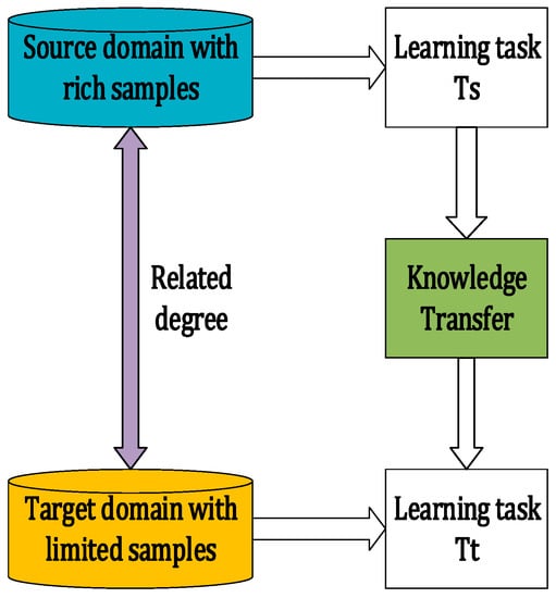
Figure 1. The concept of transfer learning.

Recent decades have witnessed the tremendous success in applying transfer learning in areas such as image recognition and sentiment analysis [10]. The prediction accuracy of the transfer learning model in the target domain relies on how related the pretrained source domain is; it is hard to find a source domain which contains enough labeled data to pretrain a prediction model of being applicable in different target domains [10]. Therefore, it is almost impossible to find a perfect source-target domain pair [11]. In order to fully explore the source domains of the related tasks, the notion of integrating the federated learning with the transfer learning is proposed. This enables the transfer learning to benefit from the federated learning based on the knowledge propagation of multiple sources of the data federation of the same industry [11,12].

The federated learning is usually regarded as the decentralized machine learning. This is closely related to multi-party preserving machine learning [13]. The federated learning can be categorized into two types: namely, vertical federated learning and horizontal federated learning with the illustration of sample complementation and feature complementation, respectively, as shown in Figure 2. The federated transfer learning enables complementary knowledge to be shared and transferred across multiple federated domains and it can be used as the extension of the conventional transfer learning task [14,15]. Recently, in order to enhance the diversity of the transfer learning, some researchers have applied federated transfer learning for practical applications. Ju et al. [16] applied federated transfer learning on the EEG (electroencephalographic) signal classification of the brain–computer interface, proving the better domain adaptation ability of the proposed federated transfer learning framework. Wang et al. [17] proposed a software heterogeneous defect prediction method based on federated transfer learning. The proposed federated transfer learning framework not only solves the problem of insufficient labels but also builds models to match the different distribution of private data. Sharma et al. [18] proposed a novel federated transfer learning framework for the knowledge integration of the scattered datasets across different organizations. These researchers have shown the great potential of the federated transfer learning in the field of knowledge integration, as well as the knowledge complementation of the transfer learning.

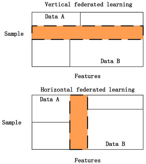
Figure 2. The vertical/horizontal federated learning.

2.2. Knowledge Distillation

The concept of knowledge distillation (KD) was first introduced by Hinton and Dean [19] as a model compression framework which releases the parameter size of the deep learning model by constructing a teacher-student paradigm where the student network is trained to capture the information contained not only in the hard version of the true label, but also in the softer version of the teacher’s output. Different from the ordinary transfer learning, the knowledge distillation accomplishes the knowledge transference tasks by altering the loss function of the student model to follow the output of the teacher model [20]. The traditional KD framework compresses one or several cumbersome networks (teachers) into a student network with a shallow structure. The framework of the conventional knowledge distillation can be categorized into two types: single teacher-based knowledge distillation and multi-teacher-based knowledge distillation [19,21,22,23,24].

2.2.1. Single Teacher-Based Distillation

Let ${\mathrm{T}}_{\mathrm{i}}$ be the output probability of the $\mathrm{ith}$ neuron of the teacher model with softmax activation ${\mathrm{T}}_{\mathrm{i}}=\frac{\exp \left({\mathrm{Z}}_{\mathrm{i}}^{\mathrm{T}}\right)}{{\sum }_{\mathrm{j}}\exp ({\mathrm{Z}}_{\mathrm{j}}^{\mathrm{T}})}$, where ${\mathrm{Z}}_{\mathrm{i}}^{\mathrm{T}}$ is the output value of the $\mathrm{ith}$ neuron before the softmax layer and j denotes the total number of the output neurons. The output probability of the $\mathrm{ith}$ neuron of the student model with softmax activation can be expressed in the same way as ${\mathrm{S}}_{\mathrm{i}}=\frac{\exp \left({\mathrm{Z}}_{\mathrm{i}}^{\mathrm{S}}\right)}{{\sum }_{\mathrm{j}}\exp ({\mathrm{Z}}_{\mathrm{j}}^{\mathrm{S}})}$. When the teacher model is used to instruct the student model, the relaxation parameter $\mathsf{\Gamma }\left(\mathsf{\Gamma }\ge 1\right)$ is introduced to the softmax layer of both networks to soften the output probability during the training process, as shown in Equation (1):

$$\begin{array}{cc}{ \mathrm{T}}_{\mathrm{i}}^{\mathsf{\Gamma }}=\frac{\exp (\raisebox{1ex}{${\mathrm{Z}}_{\mathrm{i}}^{\mathrm{T}}$}\!\left/ \!\raisebox{-1ex}{$\mathsf{\Gamma }$}\right.)}{{\sum }_{\mathrm{j}}\exp (\raisebox{1ex}{${\mathrm{Z}}_{\mathrm{i}}^{\mathrm{T}}$}\!\left/ \!\raisebox{-1ex}{$\mathsf{\Gamma }$}\right.)}, & {\mathrm{S}}_{\mathrm{i}}^{\mathsf{\Gamma }}=\frac{\exp (\raisebox{1ex}{${\mathrm{Z}}_{\mathrm{i}}^{\mathrm{S}}$}\!\left/ \!\raisebox{-1ex}{$\mathsf{\Gamma }$}\right.)}{{\sum }_{\mathrm{j}}\exp (\raisebox{1ex}{${\mathrm{Z}}_{\mathrm{i}}^{\mathrm{S}}$}\!\left/ \!\raisebox{-1ex}{$\mathsf{\Gamma }$}\right.)} \end{array}$$

(1)

Let the ${\mathrm{P}}_{\mathrm{S}}$ be the parameter of the student network and the network can be trained to optimize the loss function, as shown in Equation (2):

$${ \mathrm{L}}_{\mathrm{KD}}\left({\mathrm{P}}_{\mathrm{S}}\right)=\left(1-\mathsf{\lambda }\right){\mathrm{L}}_1\left({\mathrm{y}}_{\mathrm{true}},\mathrm{S}\right)+{\mathsf{\lambda }\mathrm{L}}_2\left({\mathrm{T}}^{\mathsf{\Gamma }},{\mathrm{S}}^{\mathsf{\Gamma }}\right)$$

(2)

As defined in Equation (2), during the training process of the single teacher-based distillation, the loss function of the student model consists of two stages where ${\mathrm{L}}_1$ and ${\mathrm{L}}_2$refer to the two-stage loss functions, respectively, and $\mathsf{\lambda }$ is an adaptive parameter of balancing the importance between both stages. It should be noted that the loss function ${\mathrm{L}}_1$ in Equation (2) enforces the student network to follow the hard labels of the ground truth while the loss function ${\mathrm{L}}_2$ enforces the student network to learn from the softened output of the teacher network. The single teacher-based knowledge distillation framework is illustrated, as shown in Figure 3:

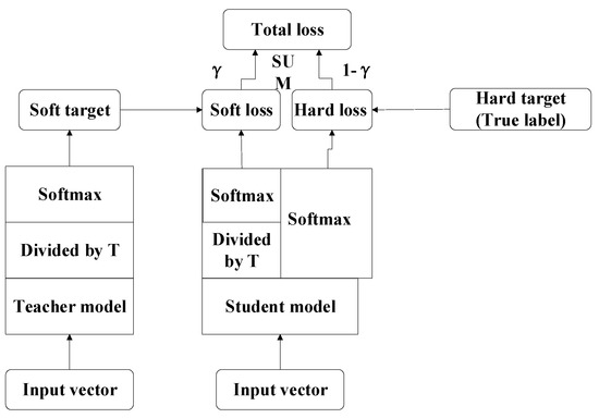
Figure 3. The single teacher-based knowledge distillation.

2.2.2. Multi-Teacher-Based Knowledge Distillation

The loss function of the student network of the multi-teacher-based knowledge distillation can be shown in Equation (3):

$${ \mathrm{L}}_{\mathrm{KD}}\left({\mathrm{W}}_{\mathrm{S}}\right)={\displaystyle \sum }_{\mathrm{i}=1}^{\mathrm{k}}{\mathrm{w}}_{\mathrm{i}}{*\mathrm{L}}_{\mathrm{i}}\left({\mathrm{T}}_{\mathrm{i}}, \mathrm{S}\right)$$

(3)

where k denotes the number of teachers and ${\mathrm{L}}_{\mathrm{i}}$ denotes the loss function between the student output and the softened label of the ith teacher output. The importance of teachers are balanced by the adaptive weight parameters of ${\mathrm{w}}_{\mathrm{i}} ,\mathrm{i}\in$(1,k) based on certain evaluation metrics. During the collaborative training process, the student model follows a group of softened labels provided by an ensemble of teachers rather than the ground truth hard label.

3. Proposed Method

3.1. Data Preprocessing

In order to satisfy the input characteristic of the CNN model, the “signal to image” conversion method based on the continuous wavelet transform (CWT) is used as the data pre-processing method in this paper, as shown in Equation (4):

$${\mathrm{CWT}}_{\mathrm{f}}\left(\mathsf{\alpha },\mathsf{\beta }\right)=⟨\mathrm{f}\left(\mathrm{t}\right),{\mathsf{\psi }}_{\mathsf{\alpha },\mathsf{\beta }}\left(\mathrm{t}\right)⟩={\left|\mathsf{\alpha }\right|}^{-\frac{1}{2}}{{\displaystyle \int }}_{-\infty }^{+\infty }\mathrm{f}\left(\mathrm{t}\right)\overline{\mathsf{\psi }}(\frac{\mathrm{t}-\mathsf{\beta }}{\mathsf{\alpha }})\mathrm{dt}$$

(4)

Given an arbitrary signal function $\mathrm{f}\left(\mathrm{t}\right)\in {\mathrm{L}}^2\left(\mathrm{R}\right)$, the continuous wavelet transform ${\mathrm{CWT}}_{\mathrm{f} }\left(\mathsf{\alpha },\mathsf{\beta }\right)$ can be expressed as the inner product between the $\mathrm{f}\left(\mathrm{t}\right)$ and the baseline wavelet function ${\mathsf{\psi }}_{\mathsf{\alpha },\mathsf{\beta }}\left(\mathrm{t}\right)$, which can be achieved by the adjustment of scale and translation, reflecting the similarity between the signal and the wavelet. $\overline{\mathsf{\psi }}\left(\mathrm{t}\right)$ denotes the conjugate of the baseline wavelet signal $\mathsf{\psi }\left(\mathrm{t}\right)$. The baseline wavelet signal can be used for accurately capturing the non-stable characteristic of the raw signal. Among all the most used baseline wavelets such as the Haar, Meyer, Mexican Hat and the Morlet, the Morlet wavelet has proved to be effective for representing the faulty symptom of the bearing vibration signal [25,26] which is used as the target wavelet in this paper. The expression function of the Morlet wavelet function can be expressed as shown in Equation (5):

$$\mathsf{\psi }\left(\mathrm{t}\right)=\exp \left(-{\mathrm{a}}^2{\mathrm{t}}^2/2\right)\cos \left(\mathsf{\pi }\mathrm{t}\right)$$

(5)

where the parameter “a” controls the shape of the Morlet wavelet and can be used for balancing the resolution between the time domain and the frequency domain. Since the Morlet wavelet transform can fully capture the signal characteristic and can achieve better resolution in both the time and frequency domain, the continuous Morlet Fourier transform is adopted in this paper for the conversion of the one-dimensional vibration signal to the two-dimensional time-frequency spectrum image. The specific process of the Morlet based “Signal to image” conversion is illustrated as shown in Figure 4. First, the window length is selected as 1024 according to the experiment of previous literature [27,28,29,30] where the 1024 continuous signal points are randomly selected each time from the raw signal. Second, the selected 1024 signal points are converted into a $1024*\mathrm{S}$ time-frequency spectrum by using the continuous Morlet wavelet transform which consists of coefficient matrices. The parameter “S” denotes the value of the scale factor $\mathsf{\alpha }$ ranging from 1 to S. Finally, the time-frequency spectrum is presented in the form of a gray-scale image.

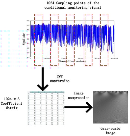
Figure 4. The Morlet based “Signal to image” conversion process.

Although more signal information can be obtained if the scale size is large enough, it is hard for the CNN to process the $1024*\mathrm{S}$ image due to its computation complexity. A simple bicubic-based interpolation-based compression method is used for shortening the image size. The size of the gray-scale image varies due to the different signal data volumes. The CWT based “Signal to Image” conversion method has already been proven to be effective in the literature [5].

3.2. Proposed FTLKD Frame Work

3.2.1. Multi Teachers Establishment Based on Federated Transfer Learning

In this section, the proposed federated transfer learning framework is proposed for the establishment of multiple teacher models. As shown in Figure 5, several offline cumbersome CNN models are first pretrained on multiple datasets that are collected from multiple related areas. After the pretrained CNN models reach certain accuracy on their own datasets, the shallow layer of the offline CNN models are transferred to several standby teacher models containing different related knowledge.

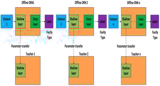
Figure 5. Multi-teacher establishment based on federated transfer learning.

3.2.2. Multi Sources Knowledge Transference Based on Knowledge Distillation

After multiple teachers are established by the federated transfer learning stated in Section 1, the established teachers containing the generalized knowledge of multiple related datasets are used as “teachers” to “guide” the student model. As shown in Figure 6, the target datasets are used for the joint training and testing of the multiple cumbersome teachers as well as the shallow structured student model. The teacher models are optimized by the hard labels provided by the datasets while the student model is optimized by multiple softened labels provided by several teacher models. The Kull-back Leibler divergence loss of the teacher model is defined here as shown in Equation (6):

$$D_{KL}(Y||\widehat{P})=\frac{1}{n}*{\displaystyle \sum }_{h=1}^n{\displaystyle \sum }_{i=1}^N\left(Y_h^i\right)*\log \left(\frac{Y_h^i}{\widehat{P_h^i}}\right)$$

(6)

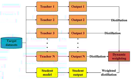
Figure 6. Multi-teacher-based online knowledge distillation.

Equation (6) denotes the Kull-back Leibler divergence loss of the teacher model where $Y_h^i$ denotes the i-th element of h-th sample of the label vector; $\widehat{P_h^i}$ denotes the ith element of the h-th sample of the output vector; N denotes the vector length and n denotes the sample number. The K-L divergence result obtained by each teacher is normalized into 0–1 as shown in Equation (7) where $\mathrm{j} (\mathrm{j}>1)$ denotes the teacher number and ${\mathrm{D}}_{{\mathrm{KL}}_{\mathrm{i}}}$ denotes the K-L divergence loss of the ${\mathrm{i}}_{\mathrm{th}}$ teacher of the current epoch:

$$x_i=\frac{D_{KLi}}{{\sum }_{i=1}^j{D}_{KLi}},{\alpha }_i=\frac{1-x_i}{j-1}$$

(7)

Since the K–L divergence value has the inverse relationship with the performance of the teacher model, the parameter ${\mathsf{\alpha }}_{\mathrm{i}}$ is defined here as the assigned weight of the ${\mathrm{i}}_{\mathrm{th}}$ teacher during the distillation process which denotes the averaging normalized K–L divergence loss of the other ($\mathrm{j}-1)$ teachers.

3.2.3. Teacher Balancing Based on KL Divergence

In this section, several teacher models are established for the weighted distillation of the student model during the training or testing process of the target datasets. The weights of the teacher models are determined according to the KL divergence loss of the current epoch of the teacher model. Since the softened output of the teacher model can provide more information for the student model so that the student model will not be over-fitted, the student models in this paper are guided by several softened teacher outputs. The specific distillation process is illustrated as shown in Equation (8):

$${ \mathrm{P}}_{{\mathrm{T}}_{\mathrm{i}}}^{\mathsf{\Gamma }}=\mathrm{softmax}\left(\frac{{\mathrm{a}}_{{\mathrm{T}}_{\mathrm{i}}}}{\mathsf{\Gamma }}\right),{ \mathrm{P}}_{\mathrm{S}}^{\mathsf{\Gamma }}=\mathrm{softmax} \left(\frac{{\mathrm{a}}_{\mathrm{S}}}{\mathsf{\Gamma }}\right)$$

(8)

where the ${\mathrm{a}}_{{\mathrm{T}}_{\mathrm{i}} }$ denotes the pre-softmax output vector of the teacher model;${\mathrm{a}}_{\mathrm{S}}$ denotes the pre-softmax output vector of the student model. A relaxation parameter $\mathsf{\Gamma }>1$ is introduced to soften the signal arising not only from the teacher output but also from the student output. The student network is trained by a group of softened teacher outputs with weight assignments as shown in Equation (9):

$${ \mathrm{L}}_{\mathrm{KD}}\left({\mathrm{W}}_{\mathrm{S}}\right)={\displaystyle \sum }_{\mathrm{i}=1}^{\mathrm{j}}{\mathsf{\alpha }}_{\mathrm{i}}*\mathrm{K}({\mathrm{P}}_{{\mathrm{T}}_{\mathrm{i}}}^{\mathsf{\Gamma }},{\mathrm{P}}_{\mathrm{S}}^{\mathsf{\Gamma }}) (\mathrm{j}>1)$$

(9)

where $\mathrm{K}(*)$ denotes the KL divergence distance between the softened corresponding teacher output and the softened student output. Parameter j denotes the total number of the guided teachers and the dynamic assigned weight ${\mathsf{\alpha }}_{\mathrm{i}}$ of the ith teacher is updated according to the KL divergence loss of the ith teacher model in the current epoch which has already been defined in Equation (6).

The KL divergence distance $\mathrm{K}(*)$ in Equation (9) is defined here as shown in Equation (10) where $y_T^i$ and $y_S^i$ denotes the ith element of the output vector of the teacher model and the student model. The parameter N denotes the vector length of the output vector

$$\mathrm{K}\left(y_T,y_S\right)={\displaystyle \sum }_{i=1}^N{y}_S^i*\log (\frac{y_T^i}{y_S^i})$$

(10)

The overall flowchart of the proposed methodology is illustrated in Algorithm 1.

Algorithm 1: General procedure of the proposed faulty prediction methodology

Input: Given the source datasets$X_S\left(x^s,y^s\right)$for the offline establishment of the teacher models and the target datasets$X_t\left(x^t,y^t\right)$for the cooperative training of the teacher models and the student model. Output: The trained student model and the faulty prediction result. Step 1: Generate the training datasets and the testing datasets Obtain the two-dimensional gray scale images of the one-dimensional time series signal by using the “signal-to-image” conversion method based on the “Continuous Wavelet Transform” as shown in Figure 4. Step 2: Construct the teacher models by using the federated transfer learning 2.1: Randomly initializing several offline CNNs and pretraining these offline CNNs on the corresponding given source datasets ${\mathrm{X}}_{\mathrm{S}}\left({\mathrm{x}}^{\mathrm{s}},{\mathrm{y}}^{\mathrm{s}}\right)$. After these offline CNN models finish training on their own source datasets, their optimized weight “W” and bias ”b” can be obtained by solving the minimum of the loss metric $\mathrm{H}\left({\mathrm{y}}_{\mathrm{true}},\widehat{{ \mathrm{y}}_{\mathrm{pre}}}\right)$ using the Adam method. 2.2: Establishing the corresponding teacher model by transferring the shallow layers of the pretrained offline CNN to the standby teacher models as shown in Figure 5, while the parameters of the other layers are randomly initialized. Step 3: Multi-teacher-based knowledge distillation 3.1: Constructing the proposed teacher-student distillation framework as shown in Figure 6. 3.2: Fine-tuning the teacher models on the training set of the target datasets ${\mathrm{X}}_{\mathrm{t}}\left({\mathrm{x}}^{\mathrm{t}},{\mathrm{y}}^{\mathrm{t}}\right)$ and calculating the KL divergence loss of the teacher model as shown in equation (6) 3.3: Dynamically update the assigned weight of teacher models during the distillation process based on the KL divergence loss of different teacher models, respectively, after each epoch as shown in equation (7). 3.4: Distilling the student model by calculating the weighted loss function between the teacher softened outputs and the student softened output as shown from equations (8) to (10). Step 4: Analysis of teacher models and the student model 4.1: Optimizing the student model through the cooperative training process by using the game strategy proposed in the literature [31,32] on the training set of the target datasets ${\mathrm{X}}_{\mathrm{t}}\left({\mathrm{x}}^{\mathrm{t}},{\mathrm{y}}^{\mathrm{t}}\right)$ during step 3 and achieve the optimized student model. 4.2: Evaluating the testing accuracy of teacher models and the student model on the testing set of the target datasets ${\mathrm{X}}_{\mathrm{t}}\left({\mathrm{x}}^{\mathrm{t}},{\mathrm{y}}^{\mathrm{t}}\right)$. Step 5: Evaluate the proposed teacher-student distillation framework. Validate the performance of the obtained student model with a different teacher-student distillation framework and output the faulty prediction results.

4. Case Studies and Experimental Result Discussion

4.1. Case Study I Bearing Faulty Prediction of the Electro-Mechanical Drive System

4.1.1. Data Description and Experimental Set Up

The performance of the proposed bearing fault prediction method is evaluated on the bearing fault datasets of the electro-mechanical drive system provided by the Paderborn University [33]. The mechanical set up of the testing rig is illustrated as shown in Figure 7 which is composed of five components marked from 1 to 5 namely a test motor; a measuring shaft; a bearing module; a flywheel and a load motor. The condition monitoring signal used in this paper is collected from the current signal of the motor. The current signal is measured by a LEM-CKSP 15-NP current transducer.. Then, the measured signal is filtered by a 25 kHz low-pass filter and converted from an analogue to a digital signal with the sampling rate of 64 kHz. The measurement systems are illustrated as shown in Figure 8.

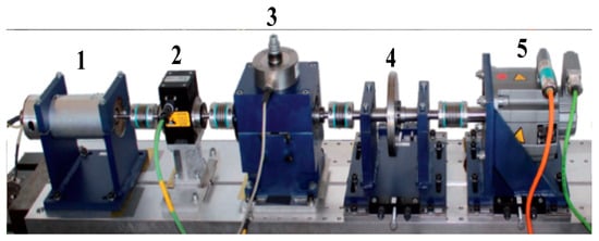
Figure 7. The testing rig of the Paderborn University.

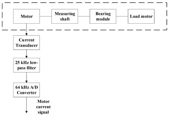
Figure 8. The measurement system of the experiment.

The collected conditional monitoring data consist of four health statuses: namely the healthy, inner-race faulty, outer-race faulty and the combined faulty. All the data are collected under the operating conditions ranging from load 0 to 3 with the parameter settings as shown in Table 1. The data collected under load 0 to 2 are regarded as the related source datasets with rich samples of 1000 in both training and testing datasets in each, respectively, while the data collected under load 3 are regarded as the target datasets with limited samples of 100 in both training and testing datasets, respectively. Each sample contains the randomly selected 1024 time series signal points. The related source datasets are used for the pretraining of the teacher models while the target datasets are used for the knowledge distillation and testing evaluation of teachers and the student. The data arrangement is illustrated as shown in Table 2:

Table 1. The operating parameters of the four operating conditions.

Loads	Rotational Speed [Rpm]	Load Torque [Nm]	Radial Force [N]	Name of Setting
0	1500	0.7	1000	N15_M07_F10
1	900	0.7	1000	N09_M07_F10
2	1500	0.1	1000	N15_M01_F10
3	1500	0.7	400	N15_M07_F04

Table 2. The data arrangement of teachers and the student.

Motor Load (HP)	Data Sample Quantity (Training/Testing)	Datasets Assignment
Load 0	1000/1000	Datasets for Teacher I
Load 1	1000/1000	Datasets for Teacher II
Load 2	1000/1000	Datasets for Teacher III
Load 3	100/100	Target datasets for Teachers & Student

4.1.2. Data Preprocessing

The one-dimensional time series current signal is transformed to the two-dimensional time-frequency spectrum through the continuous wavelet transform with the scale factor “S” of 200 which is set according to the data volumes [5]. The time-frequency spectrum is converted to the $16*16$ gray-scale image by using the bicubic interpolation. As shown in Figure 9, there is obvious distinguishable difference among these converted images of different health conditions, indicating the effectiveness of the data preprocessing method used in the literature [5] also being applicable in case study I of this paper.

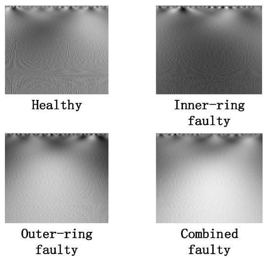
Figure 9. The conversion result of the raw current signal.

4.1.3. Offline CNN Models Set Up Based on Offline Training

In this section, three cumbersome offline CNN models are pretrained on their source datasets collected under the load conditions of load 0–2, respectively. The configuration of the teacher model is illustrated as shown in Table 3. The blocks of B1–B3 are the convolution blocks with six layers in each and they are used for hierarchical feature learning, while the last block of B4 is the faulty prediction block with the Flatten and Soft-max layers. The established cumbersome CNN models are pretrained on their own datasets and the training accuracy curves are illustrated as shown in Figure 10a–c. All of the established offline CNN models can converge with limited epochs and reach above 95% on their own datasets in terms of training and testing accuracy.

Table 3. The specific configuration of the cumbersome private model.

Block	Layer Number	Layer Type	Kernel Size	Kernel Number	Stride	Padding
B1	1	Conv	$3*3$	32	1	Same
	2	BN	-	-	-	-
	3	Conv	$3*3$	32	1	Same
	4	BN	-	-	-	-
	5	Conv	$3*3$	32	2	Same
	6	BN	-	-	-	-
B2	7	Conv	$3*3$	64	1	Same
	8	BN	-	-	-	-
	9	Conv	$3*3$	64	1	Same
	10	BN	-	-	-	-
	11	Conv	$3*3$	64	2	Same
	12	BN	-	-	-	-
B3	13	Conv	$3*3$	128	1	Same
	14	BN	-	-	-	-
	15	Conv	$3*3$	128	1	Same
	16	BN	-	-	-	-
	17	Conv	$3*3$	128	2	Same
	18	BN	-	-	-	-
B4	19	FC	1000	-	-	-
	20	Dense	32	-	-	-
	21	Softmax	4	-	-	-

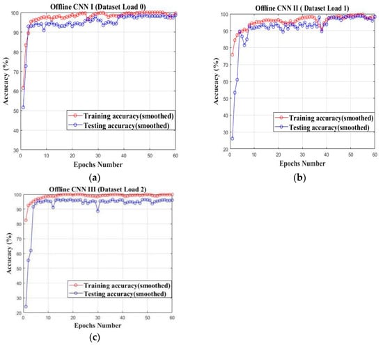
Figure 10. The offline pretraining of cumbersome private models on their own datasets: (a) Private model I (Load 0); (b) Private model II (Load 1); (c) Private model III (Load 2).

4.1.4. Teacher Establishment Based on Federated Transfer Learning

After the cumbersome private models finished offline training on their own datasets with the expected convergence accuracy, the shallow block “B1” of the offline CNN models is transferred to the online teacher models as shown in Figure 11, which is used for the following knowledge distillation. The established online teacher models are trained on the target training sets of Load 3 as illustrated in Figure 12. The KL divergence loss of the three established teachers are close to zero within the limited epochs, indicating the learning ability of the established teacher models on the target datasets.

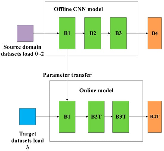
Figure 11. The establishment of the online teacher model.

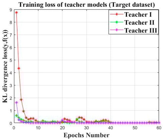
Figure 12. The training loss of the three established teacher model.

4.1.5. Knowledge Transference Based on Knowledge Distillation

In this case study, the three established teacher models are used for the knowledge transference and knowledge distillation of the student model. The configuration of the student model is illustrated as shown in Table 4 which has only one six-layer convolution block and one three-layer faulty prediction block. The student model is guided by the output of three teachers and the overall weighted loss function of the student model in this case study is illustrated as shown in Equation (11):

$${\mathrm{L}}_{\mathrm{KD}}({\mathrm{W}}_{\mathrm{S}})={\mathsf{\alpha }}_1*\mathrm{K}({\mathrm{P}}_{{\mathrm{T}}_1}^{20},{\mathrm{P}}_{\mathrm{S}}^{20})+{\mathsf{\alpha }}_2*\mathrm{K}({\mathrm{P}}_{{\mathrm{T}}_2}^{20},{\mathrm{P}}_{\mathrm{S}}^{20})+{\mathsf{\alpha }}_3*\mathrm{K}({\mathrm{P}}_{{\mathrm{T}}_3}^{20},{\mathrm{P}}_{\mathrm{S}}^{20})$$

(11)

Table 4. The configuration of the student model.

Block	Layer Number	Layer Type	Kernel Size	Kernel Number	Stride	Padding
S1	1	Conv	$3*3$	32	1	Same
	2	BN	-	-	-	-
	3	Conv	$3*3$	32	1	Same
	4	BN	-	-	-	-
	5	Conv	$3*3$	32	2	Same
	6	BN	-	-	-	-
S2	7	FC	1000	-	-	-
	8	Dense	32	-	-	-
	9	Softmax	4	-	-	-

As shown in Equation (10), the parameters ${\mathsf{\alpha }}_1,{\mathsf{\alpha }}_2$and ${\mathsf{\alpha }}_3$ denote the assigned weight of the three teacher models, respectively, which is dynamically changed according to the real time KL divergence distance between the teacher output and the true labels. The temperature parameter $\mathsf{\Gamma }$ is set for the value of 20 and the function $\mathsf{K}(*)$ denotes KL divergence between the softened student output and the corresponding teacher output. The specific knowledge distillation process is illustrated as shown in Figure 13a,b. Figure 13a denotes the dynamic weight change of three teachers within 60 epochs. It can be found that the weights of three teachers are dynamically updated after each epoch. The assigned weights of teacher I and teacher III are significantly higher than the weight of teacher II, although they are similar to each other. Therefore, it can be concluded that in case study I, the source datasets of Load 0 and Load 2 have a similar related degree with the target datasets of Load 3, while the source datasets of Load 1 have a comparatively lower related degree with the target datasets of Load 3. Figure 13b denotes the KL divergence loss between the student model and three teachers within the maximum epoch number of ⁶0th and the overall weighted loss of the student model which has already been represented in Equation (10). The KL divergence distance between each teacher output and the student output and the overall weighted loss of the student model are close to 0 within the maximum epoch, indicating the effectiveness of the proposed weighted knowledge distillation approach.

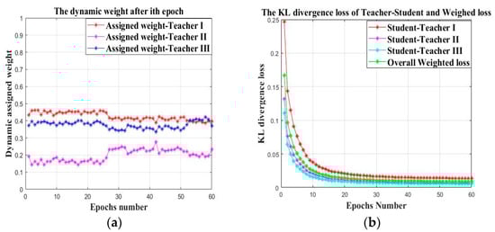
Figure 13. The dynamic knowledge distillation process of the proposed approach: (a) The changing curve of the assigned “teacher weight”; (b) The KL divergence loss of the teacher-student and the overall weighed loss.

4.1.6. Model Evaluation

After the proposed approach finishes the knowledge distillation process, the three established teacher models and the student model are validated on the testing set of the target datasets and the testing accuracy is illustrated as shown in Figure 14. All three teacher models and the student model can reach an accuracy above 95%. The experiment is repeated ten times and the average testing accuracy, the parameter size and the average KL divergence loss of three teacher models and the student model is illustrated as shown in Table 5. It should be noted that although the student model does not have the best behavior among all the models in terms of average accuracy, the student model has a comparatively smaller parameter size and a lower average KL divergence loss.

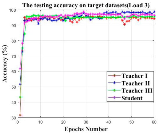
Figure 14. The testing accuracy of three teacher models and the student model.

Table 5. The average accuracy, average KL divergence loss and the parameter size of three teachers and the student.

Model	Average Accuracy (%)	Parameter Number	Average KL Divergence Loss
Teacher I	94.58%	4,677,924	3.59
Teacher II	98.13%	4,677,924	0.77
Teacher III	95.44%	4,677,924	0.47
Student	96.69%	1,142,764	0.02

4.1.7. Comparison with Other Distillation Frameworks

In order to further evaluate the effectiveness of the proposed approach, multiple knowledge distillation frameworks with different arrangement of teachers and source datasets are introduced for comparison. The specific detail is illustrated in Table 6. As shown in Table 6, case I is the knowledge distillation framework proposed in the paper where the student model is guided by three teachers; cases II–IV represent the framework where the students are guided by only two teachers; cases V–VII represent the framework where the students are guided by only one teacher, which is the same as the single teacher-based distillation referred in Section 2. The single teacher-based distillation regulation used for comparison here is illustrated as shown in Equation (12), where the ${\mathrm{D}}_{\mathrm{KL}}({\mathrm{Q}}_{\mathrm{T}}||{\mathrm{y}}_{\mathrm{true}})$ denotes the KL divergence loss of the teacher model in the current epoch. The ${\mathrm{D}}_{\mathrm{KL}}{({\mathrm{Q}}_{\mathrm{T}}||{\mathrm{y}}_{\mathrm{true}})}_{\max }$ denotes the maximum KL divergence distance of the teacher model within the 60 epochs. In case VIII, there is no teacher guidance and the student model is directly trained and tested on the training/testing set of the target datasets that were collected under Load 3.

$$L_{KD}\left(W_S\right)=\lambda *H\left(y_{true},P_S\right)+\left(1-\lambda \right)*H\left(P_{T_i}^{\mathsf{\Gamma }},P_S^{\mathsf{\Gamma }}\right), \lambda =\frac{D_{KL}(Q_T||y_{true})}{D_{KL}{(Q_T||y_{true})}_{max}}$$

(12)

Table 6. Details of guiding teachers used for knowledge distillation in different cases.

Method	Teacher Number	Datasets I (Load 0)	Datasets II (Load 1)	Datasets III (Load 2)
Case I	3	Teacher 1	Teacher 2	Teacher 3
Case II	2	Teacher 1	Teacher 2
Case III	2		Teacher 2	Teacher 3
Case IV	2	Teacher 1		Teacher 3
Case V	1	Teacher 1
Case VI	1		Teacher 2
Case VII	1			Teacher 3
Case VIII	0	No teacher

The student models trained by each case are evaluated on the testing set of the target datasets with a different knowledge distillation framework, as shown in Figure 15. The student model guided by three teacher models in case I has the highest testing accuracy on the target datasets (approximately 95%); the student models guided by two teachers in cases II–IV have a testing accuracy of approximately 90%; the student models guided by only one teacher in cases V–VII have a testing accuracy of approximately 80%; the student model with no teacher guidance in case VIII has the lowest testing accuracy of approximately 65%. The reason for this should be that the student model guided by more teachers can obtain more diversity prior knowledge from the related source domain areas which can promote the learning ability of the student model on target datasets.

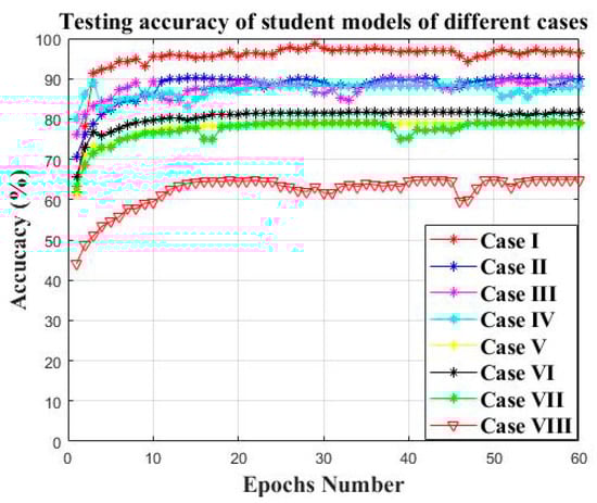
Figure 15. The testing accuracy of student models of different cases on target datasets.

The experiment is repeated 10 times. The average testing accuracy and the average KL divergence loss of the student models of different cases are illustrated in Table 7. The student model that was guided by more teachers can obtain a higher accuracy and lower KL divergence loss, indicating the effectiveness of the combination of the federated transfer learning and knowledge distillation.

Table 7. The average accuracy and KL divergence loss of student models on target testing datasets under different cases.

Method	Average Testing Accuracy	Average KL Divergence Loss
Case I	96.69%	0.02
Case II	88.07%	0.048
Case III	87.65%	0.051
Case IV	87.05%	0.093
Case V	77.73%	0.339
Case VI	80.47%	0.675
Case VII	79.35%	0.474
Case VIII	62.19%	10.115

4.1.8. Comparison with Other Machine Learning Models

The proposed federated transfer learning and knowledge distillation network which consists of three teacher models and one student model are compared with other traditional machine learning approaches such as BPNN, SVM, DAE and DBN. The experiment is arranged as follows: The student model has the prior knowledge of being guided by three teachers; teachers I–III have the prior knowledge of being pre-trained on datasets I–III of case study I. The traditional machine learning models of DAE, BPNN, DBN, SVM and CNN do not have prior knowledge and are directly trained and tested on the target datasets. It should be noted that the CNN used as the traditional machine learning model has the same structure as the teacher model. The comparison experiment is repeated ten times and the mean accuracy and the KL divergence loss are illustrated as shown in Table 8. It can be found that the student model and three teacher models with prior knowledge can achieve a higher testing accuracy and lower testing loss on the target datasets when compared with other traditional machine learning models. The problem is that it is hard for traditional machine learning models to perform well on small sampled datasets without prior knowledge, indicating the importance of prior knowledge under the limited labeled data.

Table 8. The comparison with other machine learning models.

Method	Prior Knowledge	Average Testing Accuracy	Average Testing Loss (KL Divergence Loss)
Student model	Guided by three teachers	96.69%	0.02
Teacher I	Pre-trained on Datasets I	94.58%	3.59
Teacher II	Pre-trained on Datasets II	98.13%	0.77
Teacher III	Pre-trained on Datasets III	95.44%	0.49
DAE	No prior knowledge	91.31%	14.27
BPNN	No prior knowledge	81.31%	10.66
DBN	No prior knowledge	89.17%	15.31
SVM	No prior knowledge	82.62%	15.94
CNN (Structure of teacher model)	No prior knowledge	87.66%	15.12

4.2. Case Study II: Bearing Faulty Prediction for Reliance Electric Motor

4.2.1. Data Description and Experimental Set Up

In case study II, the proposed faulty prediction methodology is evaluated on the bearing faulty datasets offered by the Case Western Reserve University (CWRU) Bearing Center [34]. The vibration signal datasets being tested here are collected from the drive-end of a 2-hp reliance electric motor under load conditions ranging from 0 to 3 with five inner-race conditional statuses of Normal; Faulty diameter 0.007; Faulty diameter 0.014; Faulty diameter 0.021 and Faulty diameter 0.028, respectively. The data arrangement is illustrated as shown in Table 9.

Table 9. The data arrangement of teachers and the student of case study II.

Rotating Speed (rpm)	Data Sample Quantity (Training/Testing)	Datasets Assignment
Load 0 (1730 rpm)	1000/1000	Datasets for teacher I
Load 1 (1750 rpm)	1000/1000	Datasets for teacher II
Load 2 (1772 rpm)	1000/1000	Datasets for teacher III
Load 3 (1797 rpm)	100/100	Datasets for teacher IV

4.2.2. Data Preprocessing

The one-dimensional current signal is transformed to the two-dimensional gray scale image through the continuous wavelet transform with the scale factor “S” of 200. As shown in Figure 16, there is also a distinguishable difference among the different conditional statuses of case study II. Since case study I is the prediction of the faulty type of different components while case study II is the prediction of the faulty severity of a certain component, the proposed approach proved to be applicable for the faulty prediction tasks of not only faulty type, but also of faulty intensity.

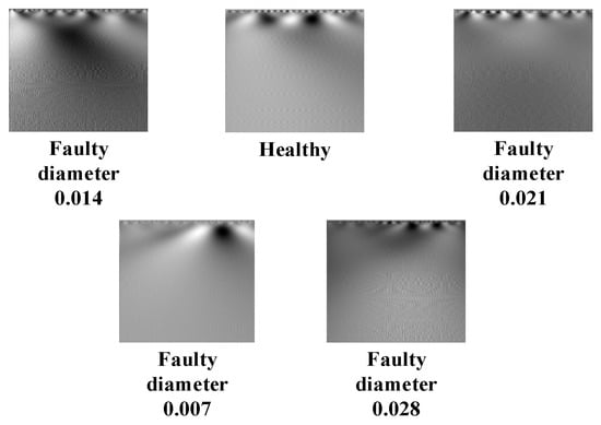
Figure 16. The conversion result of the raw current signal under load 0.

4.2.3. Private Models Establishment Based on Offline Private Training

The three cumbersome models are set up and pre-trained on the private datasets of loads 0–2, respectively. As shown in Figure 17a–c, the established private models in case study II can also converge within limited epochs and reach an accuracy of approximately 100% on their own datasets in terms of training and testing accuracy.

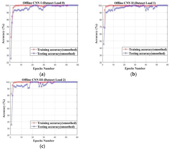
Figure 17. The offline pretrain of cumbersome private models on their own datasets on case study II: (a) Private model I (Load 0); (b) Private model II (Load 1); (c) Private model III (Load 2).

4.2.4. Teacher Establishment Based on Federated Transfer Learning

After the cumbersome private models finish offline training on their own private datasets, the shallow layers of the cumbersome private models are transferred to the low layer of the online teacher models as the transfer process of case study I which has already been illustrated in Figure 10. As illustrated in Figure 18, the three established online teacher models are trained on the target training set of Load 3. In addition, the KL divergence loss of the three online teachers is close to zero within the limited epochs, indicating the learning ability of the established teacher models in case study II.

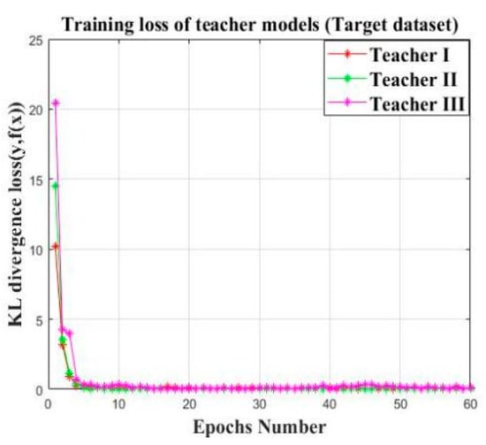
Figure 18. The target training loss of the three established teacher models.

4.2.5. Knowledge Transference Based on Knowledge Distillation

As in case study I, the three established teacher models are used for the knowledge transference and knowledge distillation of the student model whose configuration has already been illustrated in Table 4 of case study I. The dynamic curve of the assigned weights of the three teachers, the KL divergence loss of the teacher-student, and the overall weighted loss are illustrated as shown in Figure 19a,b. As shown in Figure 19a, there is no obvious difference among the three teachers in terms of the assigned weight of case study II. Therefore, it can be concluded that the source domain datasets of Loads 0–2 have a similar related degree with the target datasets of Load 3 in case study II which is different from case study I. The KL divergence loss of the three teacher-student pairs and the overall weighted loss of the student model are illustrated in Figure 19b. It can be found that all the curves are close to zero within the maximum epoch range of 60, indicating that the proposed knowledge distillation approach is also applicable in case study II.

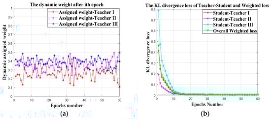
Figure 19. The dynamic knowledge distillation process of the proposed approach: (a) The changing curve of the assigned “teacher weight”; (b) The KL divergence loss of the teacher-student and the overall weighted loss.

4.2.6. Model Evaluation

After completing the knowledge distillation process, the three established teacher models and the student model are performed on the testing set of the target datasets of case study II. As shown in Figure 20 and Table 10 in case study II, the student model outperforms the three teacher models in terms of both the average prediction accuracy and the average KL-divergence loss with a smaller parameter size.

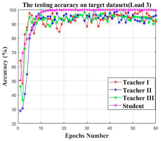
Figure 20. The testing accuracy of three teacher models and the student model.

Table 10. The average accuracy and the parameter size of three teachers and the student.

Model	Average Accuracy (%)	Parameter Size	Average KL Divergence Loss
Teacher I	95.12%	4,677,924	2.63
Teacher II	94.63%	4,677,924	3.59
Teacher III	94.81%	4,677,924	5.73
Student	99.83%	1,142,764	0.076

4.2.7. Comparison with Other Distillation Frameworks

The simulation result of the comparison study of case study II is illustrated as shown in Figure 21 and Table 11. The performance of the student model becomes better with the increase in teacher models, indicating the effectiveness of introducing the multi sources federated transfer learning into the knowledge distillation.

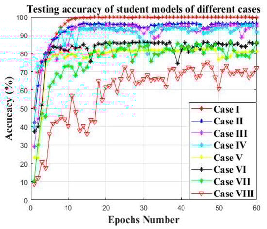
Figure 21. The testing accuracy of student models of different cases.

Table 11. The average accuracy and KL divergence loss of student models on the target testing datasets under different cases.

Method	Average Accuracy	Average KL Divergence Loss
Case I	99.83%	0.076
Case II	93.04%	0.094
Case III	90.04%	0.171
Case IV	91.07%	0.114
Case V	78.08%	1.154
Case VI	82.01%	1.782
Case VII	76.27%	2.796
Case VIII	58.74%	12.919

4.2.8. Comparison with Other Machine Learning Models

Similar to Section 4.1.8, the comparison experiment with other machine learning models is repeated ten times. The mean accuracy and the KL divergence loss is illustrated as shown in Table 12. In case study II, under the limited labeled dataset, the student model and three teacher models with prior knowledge can achieve higher testing accuracy and lower testing loss on the target datasets when compared with other traditional machine learning models.

Table 12. The comparison with other machine learning models.

Method	Prior Knowledge	Average Testing Accuracy	Average Testing Loss
Student model	Guided by three teachers	99.83%	0.076
Teacher I	Pre-trained on load 0	95.12%	2.63
Teacher II	Pre-trained on load 1	94.63%	3.59
Teacher III	Pre-trained on load 2	94.81%	5.73
DAE	No prior knowledge	78.45%	10.38
BPNN	No prior knowledge	86.58%	11.56
DBN	No prior knowledge	87.55%	9.92
SVM	No prior knowledge	81.45%	6.21
CNN (structure of teacher model)	No prior knowledge	90.45%	7.18

5. Contribution and Future Work

5.1. Main Contribution of This Paper

In this paper, a novel hybrid-bearing faulty prediction method based on the federated transfer learning and knowledge distillation is proposed. The main contributions of this paper can be summarized as follows:

(1)

The “signal to image” conversion method based on the continuous wavelet transform in the literature [5] is introduced to the data pre-processing of this paper which can well represent the information of machine health conditions contained in the raw signal.

(2)

Proposing a novel federated transfer learning framework (FTL) which contains prior knowledge from multiple different but related source domain areas. Several cumbersome models are pretrained on the datasets of multiple related areas, contributing different knowledge for the knowledge compensation of the transfer learning. The performance of the federated transfer learning model will not rely on a single source domain, enhancing the model’s generalization ability.

(3)

Proposing a novel multi-teacher-based knowledge distillation (KD) framework. The student model is guided by several teachers and the teacher models are dynamically weighted based on the real time KL divergence loss between the teacher output and the true label. The student model can obtain knowledge from different teachers with a lower parameter size which can be applicable for the edge computing-based deployment.

The two case studies illustrated in this paper show that the student model trained by the proposed knowledge distillation framework can obtain higher testing accuracy on target datasets with lower KL divergence loss and a smaller parameter size.

5.2. Future Work of This Paper

Although the proposed approach has made some achievements, three limitation issues still require consideration in our future work:

(1)

In this paper, the proposed federated transfer model is constructed based on the set up of multiple teacher models; however, it is laborious and costly to pretrain multiple teachers from different but related areas. Moreover, the weight assignment of the teacher models will become complicated with the increase in teacher models;

(2)

In this paper, the “Knowledge” learned by multiple teacher models from multiple related datasets are more likely to represent the basic features of multiple datasets. Further, the whole process of knowledge learning and knowledge transference is entirely based on the black-box theory, indicating that it is not able to be explained.

(3)

In this paper, the proposed bearing faulty prediction only offers the conditional prediction of the bearing status. However, it has not been extended to the determination of the maintenance strategy which might be more meaningful to the practical industry.

In the future, some simplifying methods will be introduced to the proposed approach for the enhancement of the model’s flexibility. Moreover, the explainable AI will be explored and adopted in the proposed faulty prediction method. Further, the explainable AI will be utilized for a deeper analysis regarding the creation of an appropriate maintenance strategy.

References

- Yaguo, L.; Naipeng, L.; Liang, G.; Ningbo, L.; Tao, Y.; Jing, L. Machinery health prognostics: A systematic review from data acquisition to RUL prediction. Mech. Syst. Signal Process. 2018, 104, 799–834. [Google Scholar]
- Peng, K.; Jiao, R.; Dong, J.; Yanting, P. A deep belief network based health indicator construction and remaining useful life prediction using improved particle filter. Neurocomputing 2019, 361, 19–28. [Google Scholar] [CrossRef]
- Shao, H.; Jiang, H.; Zhang, H.; Liang, T. Electric Locomotive Bearing Fault Diagnosis Using a Novel Convolutional Deep Belief Network. IEEE Trans. Ind. Electron. 2017, 65, 2727–2736. [Google Scholar] [CrossRef]
- Chen, Z.; Li, W. Multi-sensor Feature Fusion for Bearing Fault Diagnosis Using Sparse Autoencoder and Deep Belief Network. IEEE Trans. Instrum. Meas. 2017, 66, 1693–1702. [Google Scholar] [CrossRef]
- Xu, G.; Liu, M.; Jiang, Z.; Söffker, D.; Shen, W. Bearing Fault Diagnosis Method Based on Deep Convolutional Neural Network and Random Forest Ensemble Learning. Sensors 2019, 19, 1088. [Google Scholar] [CrossRef] [Green Version]
- Xiao, D.; Huang, Y.; Qin, C. Transfer learning with convolutional neural networks for small sample size problem in machinery fault diagnosis. Arch. Proc. Inst. Mech. Eng. Part C J. Mech. Eng. Sci. 2019, 233, 5131–5143. [Google Scholar] [CrossRef]
- Cao, P.; Zhang, S.; Tang, J. Pre-Processing-Free Gear Fault Diagnosis Using Small Datasets with Deep Convolutional Neural Network-Based Transfer Learning. IEEE Access 2017, 6, 26241–26253. [Google Scholar] [CrossRef]
- Han, T.; Liu, C.; Yang, W.; Jiang, D. Deep Transfer Network with Joint Distribution Adaptation: A New Intelligent Fault Diagnosis Framework for Industry Application. ISA Trans. 2019, 97, 269–281. [Google Scholar] [CrossRef] [Green Version]
- Wen, L.; Gao, L.; Li, X. A New Deep Transfer Learning Based on Sparse Auto-Encoder for Fault Diagnosis. IEEE Trans. Syst. Man Cybern. Syst. 2019, 49, 136–144. [Google Scholar] [CrossRef]
- Wang, C.; Mahadevan, S. Heterogeneous Domain Adaptation Using Manifold Alignment. In Proceedings of the International Joint Conference on IJCAI, DBLP, Barcelona, Spain, 16–22 July 2011. [Google Scholar]
- Liu, Y.; Kang, Y.; Xing, C.; Chen, T.; Yang, Q. A Secure Federated Transfer Learning Framework. Intell. Syst. IEEE 2020, 35, 70–82. [Google Scholar] [CrossRef]
- Huang, T.; Lin, W.; Wu, W.; He, L.; Li, K.; Zomaya, A.Y. An Efficiency-boosting Client Selection Scheme for Federated Learning with Fairness Guarantee. IEEE Trans. Parallel Distrib. Syst. 2020, 32, 1552–1564. [Google Scholar] [CrossRef]
- Szepesvári, C. Synthesis Lectures on Artificial Intelligence and Machine Learning; Morgan & Claypool: San Rafael, CA, USA, 2019. [Google Scholar]
- Yang, Q. Federated learning: The last on kilometer of artificial intelligence. CAAI Trans. Intell. Syst. 2020, 15, 183–186. [Google Scholar]
- McMahan, H.B.; Moore, E.; Ramage, D.; Arcas, B.A. Federated Learning of Deep Networks using Model Averaging. arXiv 2016, arXiv:1602.05629. [Google Scholar]
- Ju, C.; Gao, D.; Mane, R.; Tan, B.; Liu, Y.; Guan, C. Federated Transfer Learning for EEG Signal Classification. In Proceedings of the 2020 42nd Annual International Conference of the IEEE Engineering in Medicine & Biology Society (EMBC), Montreal, QC, Canada, 20–24 July 2020. [Google Scholar]
- Wang, A.; Zhang, Y.; Yan, Y. Heterogeneous Defect Prediction Based on Federated Transfer Learning via Knowledge Distillation. IEEE Access 2021, 9, 29530–29540. [Google Scholar] [CrossRef]
- Sharma, S.; Xing, C.; Liu, Y.; Kang, T. Secure and Efficient Federated Transfer Learning. In Proceedings of the 2019 IEEE International Conference on Big Data (Big Data), Los Angeles, CA, USA, 9–12 December 2019. [Google Scholar]
- Hinton, G.; Dean, J.; Vinyals, O. Distilling the Knowledge in a Neural Network. arXiv 2014, arXiv:1503.02531. [Google Scholar]
- Alkhulaifi, A.; Alsahli, F.; Ahmad, I. Knowledge distillation in deep learning and its applications. PeerJ Comput. Sci. 2021, 7, e474. [Google Scholar] [CrossRef]
- Romero, A.; Ballas, N.; Kahou, S.E.; Chassang, A.; Bengio, Y. FitNets: Hints for Thin Deep Nets. arXiv 2015, arXiv:1412.6550. [Google Scholar]
- Markov, K.; Matsui, T. Robust Speech Recognition Using Generalized Distillation Framework. Interspeech 2016, 2364–2368. [Google Scholar] [CrossRef]
- Chebotar, Y.; Waters, A. Distilling Knowledge from Ensembles of Neural Networks for Speech Recognition. Interspeech 2016, 3439–3443. [Google Scholar] [CrossRef] [Green Version]
- Yuan, M.; Peng, Y. CKD: Cross-Task Knowledge Distillation for Text-to-Image Synthesis. IEEE Trans. Multimed. 2020, 22, 1955–1968. [Google Scholar] [CrossRef]
- Huang, S.J.; Hsieh, C.T. High-impedance fault detection utilizing a morlet wavelet transform approach. IEEE Trans. Power Deliv. 1999, 14, 1401–1410. [Google Scholar] [CrossRef]
- Lin, J.; Liangsheng, Q.U. Feature Extraction Based on Morlet Wavelet and Its Application for Mechanical Fault Diagnosis. J. Sound Vib. 2000, 234, 135–148. [Google Scholar] [CrossRef]
- Sun, J.; Yan, C.; Wen, J. Intelligent Bearing Fault Diagnosis Method Combining Compressed Data Acquisition and Deep Learning. IEEE Trans. Instrum. Meas. 2017, 67, 185–195. [Google Scholar] [CrossRef]
- Long, W.; Xinyu, L.; Gao, L.; Zhang, Y. A New Convolutional Neural Network-Based Data-Driven Fault Diagnosis Method. IEEE Trans. Ind. Electron. 2017, 65, 5990–5998. [Google Scholar]
- Min, X.; Teng, L.; Lin, X.; Liu, L.; de Silva, C.W. Fault Diagnosis for Rotating Machinery Using Multiple Sensors and Convolutional Neural Networks. IEEE/ASME Trans. Mechatron. 2017, 23, 101–110. [Google Scholar]
- Ding, X.; He, Q. Energy-Fluctuated Multi-scale Feature Learning With Deep ConvNet for Intelligent Spindle Bearing Fault Diagnosis. IEEE Trans. Instrum. Meas. 2017, 66, 1926–1935. [Google Scholar] [CrossRef]
- Wong, K. Bridging game theory and the knapsack problem: A theoretical formulation. J. Eng. Math. 2015, 91, 177–192. [Google Scholar] [CrossRef]
- Wong, K. A Geometrical Perspective for the Bargaining Problem. PLoS ONE 2010, 5, e10331. [Google Scholar] [CrossRef] [Green Version]
- Lessmeier, C.; Kimotho, J.K.; Zimmer, D.; Sextro, W. Condition Monitoring of Bearing Damage in Electromechanical Drive Systems by Using Motor Current Signals of Electric Motors: A Benchmark Data Set for Data-Driven Classification. In Proceedings of the European Conference of the PHM Society, Bilbao, Spain, 5–8 July 2016; Volume 3. [Google Scholar] [CrossRef]
- Loparo, K. Case Western Reserve University Bearing Data Centre Website. 2012. Available online: https://engineering.case.edu/bearingdatacenter/12k-drive-end-bearing-fault-data (accessed on 12 December 2018).
Publisher’s Note: MDPI stays neutral with regard to jurisdictional claims in published maps and institutional affiliations. |
© 2022 by the authors. Licensee MDPI, Basel, Switzerland. This article is an open access article distributed under the terms and conditions of the Creative Commons Attribution (CC BY) license (https://creativecommons.org/licenses/by/4.0/).