Article

A New Piecewise Nonlinear Asymmetry Bistable Stochastic Resonance Model for Weak Fault Extraction

Department of Mechanical Engineering, Shanghai Polytechnic University, Shanghai 201209, China
*
Author to whom correspondence should be addressed.
Machines 2022, 10(5), 373; https://doi.org/10.3390/machines10050373
Submission received: 4 April 2022 / Revised: 10 May 2022 / Accepted: 12 May 2022 / Published: 14 May 2022
(This article belongs to the Special Issue Advances in Bearing Modeling, Fault Diagnosis, RUL Prediction)

Abstract

:
In order to solve output saturation problems found in traditional stochastic resonance methods and to improve the diagnosis ability of weak faults, a new piecewise nonlinear asymmetric bistable stochastic resonance (PNABSR) method is proposed. This model uses a left and right potential function with an asymmetrical shape, which makes it easier to induce stochastic resonance phenomena. Based on the PNABSR model, the expression of the signal-to-noise ratio (SNR) is derived, and the changes in the SNR with different parameters in the PNABSR model are analyzed. Then, the parameters in the PNABSR model are optimized using the adaptive intelligent algorithm to enhance the diagnostic ability. The diagnosis properties of the weak fault are compared between the PNABSR model and the classical bistable stochastic resonance model (CBSR). The experimental results prove that the PNABSR model can effectively extract the weak fault characteristic frequency under a strong noise background, verifying the effectiveness of this method.

1. Introduction

The stochastic resonance (SR) signal processing method uses noise to enhance useful weak signals, which is helpful for extracting and detecting weak signals under low SNR conditions. Benzi et al. [1] used the stochastic resonance method to predict periodic alternations during warm climate periods. According to this theory, a moderate amount of noise can enhance the modulation ability of weak signals to the nonlinear system. Subsequently, the concept of stochastic resonance is applied to enhance noise performance [2]. At present, the random facilitation effect has been proposed to explain the increase in the system output response under the combined action of nonlinear systems, noise, and lower frequency signals [3]. Fauve and Heslot [4] added a modulated signal and noise signal to the Schmitt trigger circuit system and found that it had an obvious peak as the noise intensity changed. This was the first time that the SR phenomenon was verified through experiments. McNamara and Wiesenfeld [5] discovered the SR phenomenon by conducting acousto-optic modulation experiments with ring lasers. Then, a classical bistable SR (CBSR) model was applied to the fault feature extraction of a weak fault signal [6]. However, inherent output saturation is a disadvantage of the CBSR model, as it reduces the output signal-to-noise ratio (SNR) and limits the model’s fault diagnosis capability [7,8].
At present, some scholars have put forward optimization and improvement methods for the CBSR model. Wang [9] proposed a new piecewise linear stochastic resonance model for detecting weak signals in a strong noise background with large parameters. This proved that it is easier to adjust the response characteristic of the system and to generate the SR in the case of large parameters. In order to further improve the signal-to-noise ratio, Qiao [10] proposed a new piecewise bistable potential model by improving the original potential function via restriction of the movement of traditional stochastic resonance particles into a piecewise second-order potential function. This method was proven capable of extracting weak fault characteristics and enhancing the anti-noise capability. Subsequently, the piecewise nonlinear bistable system (PNBSR) model was proposed to overcome the saturation characteristics of the CBSR model [11]. However, the potential functions of the PNBSR and CBSR models are same. Tang [12] proposed an improved piecewise mixed stochastic resonance (PMSR) potential model. The fourth-order potential function in the PNBSR model was improved to a piecewise second-order potential function. Experiments proved that this model can accurately extract weak fault features, thereby showing effects that were better than those obtained using the PNBSR method.
Recently, other piecewise stochastic resonance models have also been proposed. Zhao [13] proposed a piecewise tri-stable stochastic resonance (PTSR) method. Experiments proved that the output signal of this method has a larger signal amplitude and a higher SNR. Huang [14] presented a piecewise bistable energy harvester model. The SNR of the piecewise bistable systems were studied. The evaluation of the piecewise bistable energy harvesters was carried out by employing the measured input signal and showed that piecewise bistable energy harvesters with a small piecewise slope perform satisfactorily under ultralow frequency excitation conditions. Recently, an asymmetric piecewise stochastic resonance model was also studied. Xu [15] studied an asymmetric tri-stable stochastic resonance model. It was found that the fault detection performance could be effectively improved by exploiting the asymmetry feature. In addition to studying the SR model, the parameters in the model can also improve performance after optimization. Liu [16] optimized the system parameters using the improved artificial fish swarm algorithm based on the adaptive SR theory. This experiment proved that the optimized SR model performed better when detecting weak signal characteristics than traditional adaptive SR in a bistable model. Above all, the piecewise SR model and asymmetric SR model have gradually attracted attention due to improvements in their weak signal detection abilities. However, an asymmetric piecewise nonlinear stochastic resonance model with parameter optimization has not yet been implemented.
Therefore, in order to overcome the shortcomings of traditional methods and to improve the weak fault signal extraction ability, further studies on asymmetric piecewise SR models and on the optimization of asymmetric potential function parameters to obtain the maximum SNR are particularly important. In-depth research should be carried out to achieve a comprehensive understanding of the asymmetric stochastic resonance model with parameter optimization.
In this paper, a new piecewise nonlinear asymmetric bistable stochastic resonance method (PNABSR) is proposed. Then, the PNABSR model is used to extract the weak fault signals of the rolling bearings. The superiority of the proposed method is compared with the CBSR model and is verified through experiments.

2. Piecewise Nonlinear Asymmetric Bistable Stochastic Resonance Model

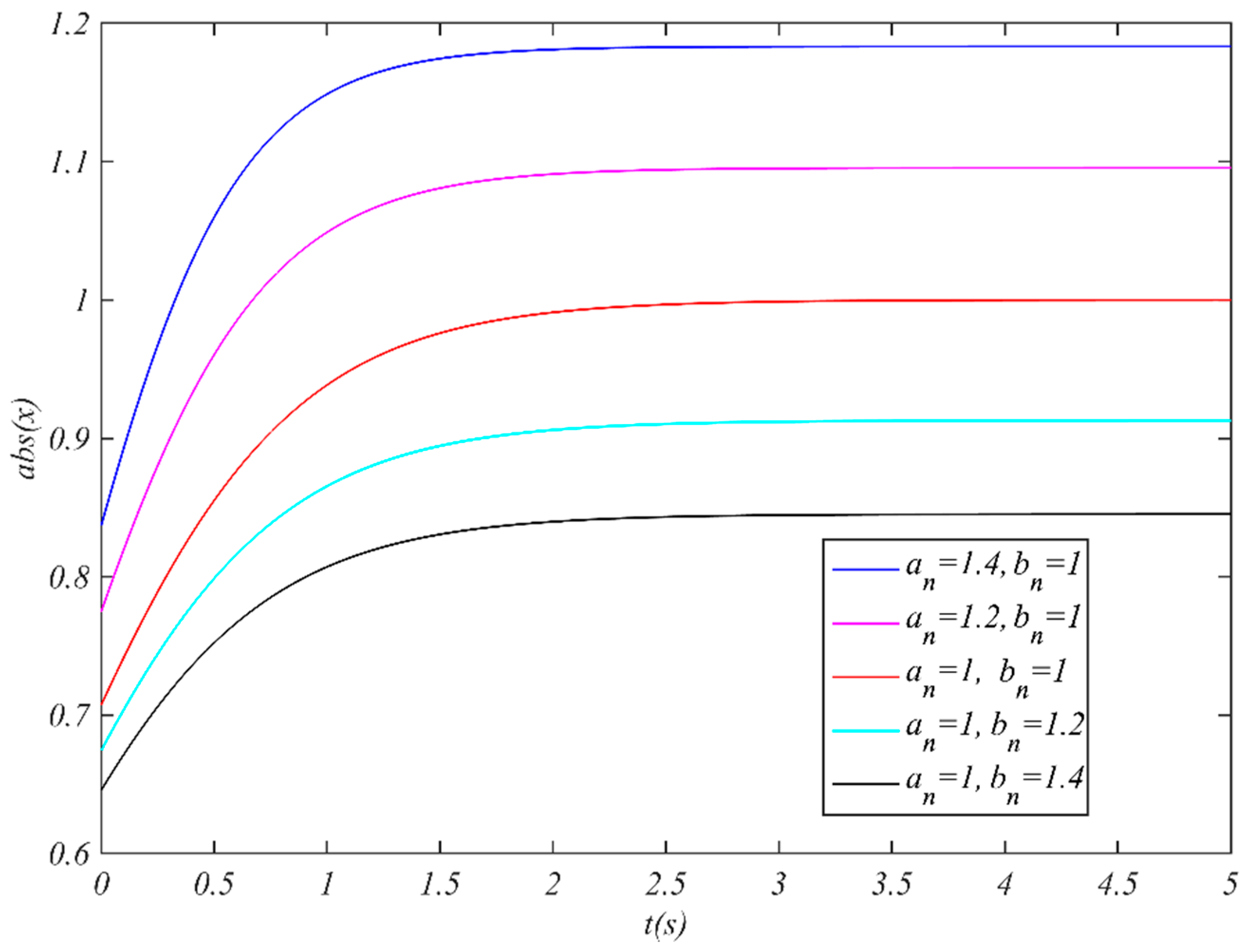
2.1. The Saturation Phenomena of CBSR Model

The Langevin equation (LE) of the CBSR is as follows [17]:
d x d t = d U n ( x ) d x + A c o s ( 2 π f 0 t ) + γ ( t )
where U n ( x ) = 1 2 a n x 2 + 1 4 b n x 4 ; A and f 0 are the amplitude and the characteristic frequency of the input signal; and γ ( t ) is additive white Gaussian noise. In Equation (2), D is the noise intensity, and φ is the time interval.
{ γ ( t ) = 0 γ ( t ) γ ( t φ ) = 2 D δ ( t )
In Equation (1), A = 0, D = 0. x(t) is obtained from the following equation [18]:
x ( t ) = ± a n b n + e 2 a n t
Figure 1 shows the effect of the parameters of the CBSR model on the saturation phenomenon. It can be seen that the output signal x(t) gradually stabilizes as time changes. This is the saturation phenomenon found in traditional stochastic resonance.

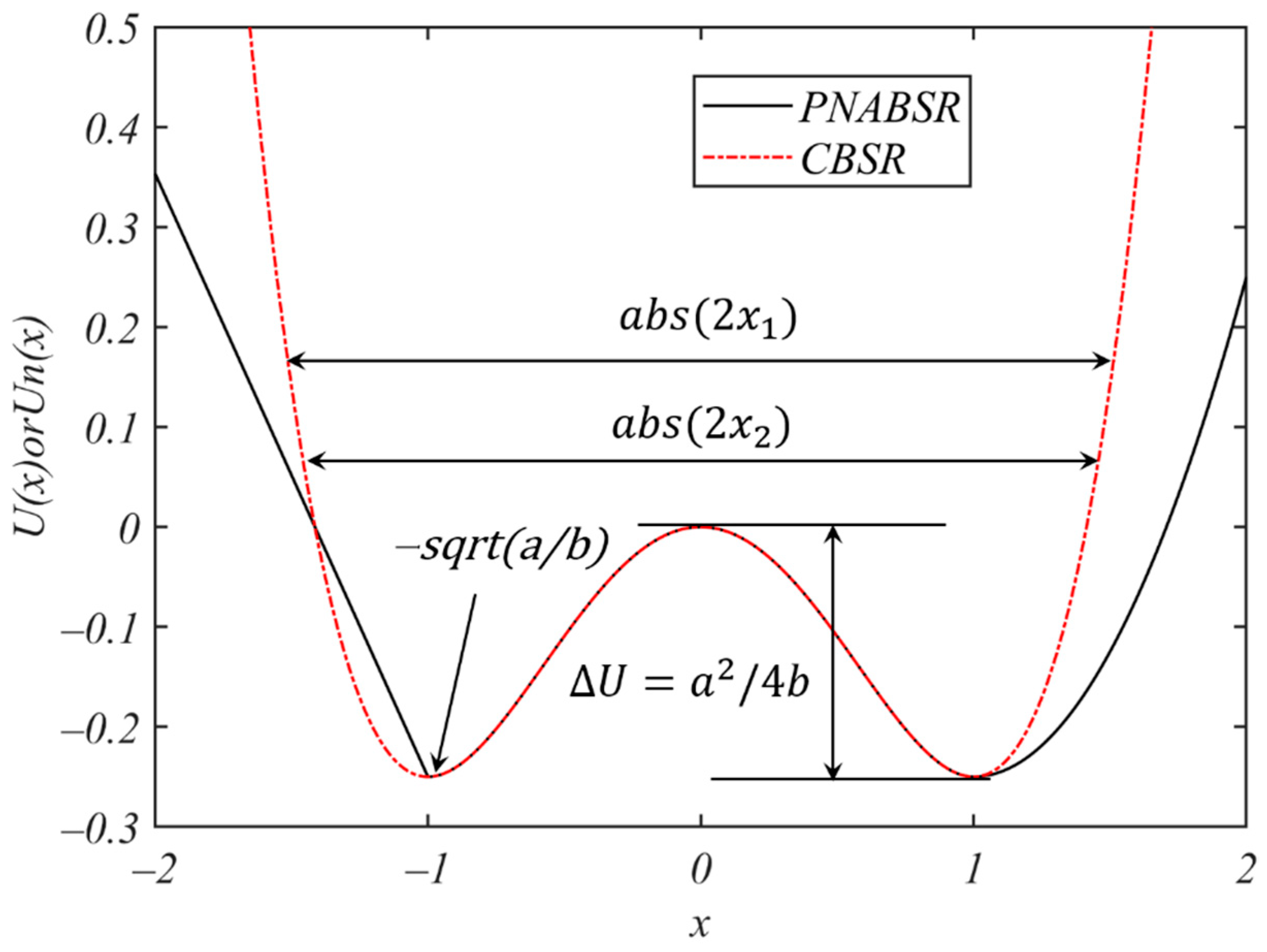
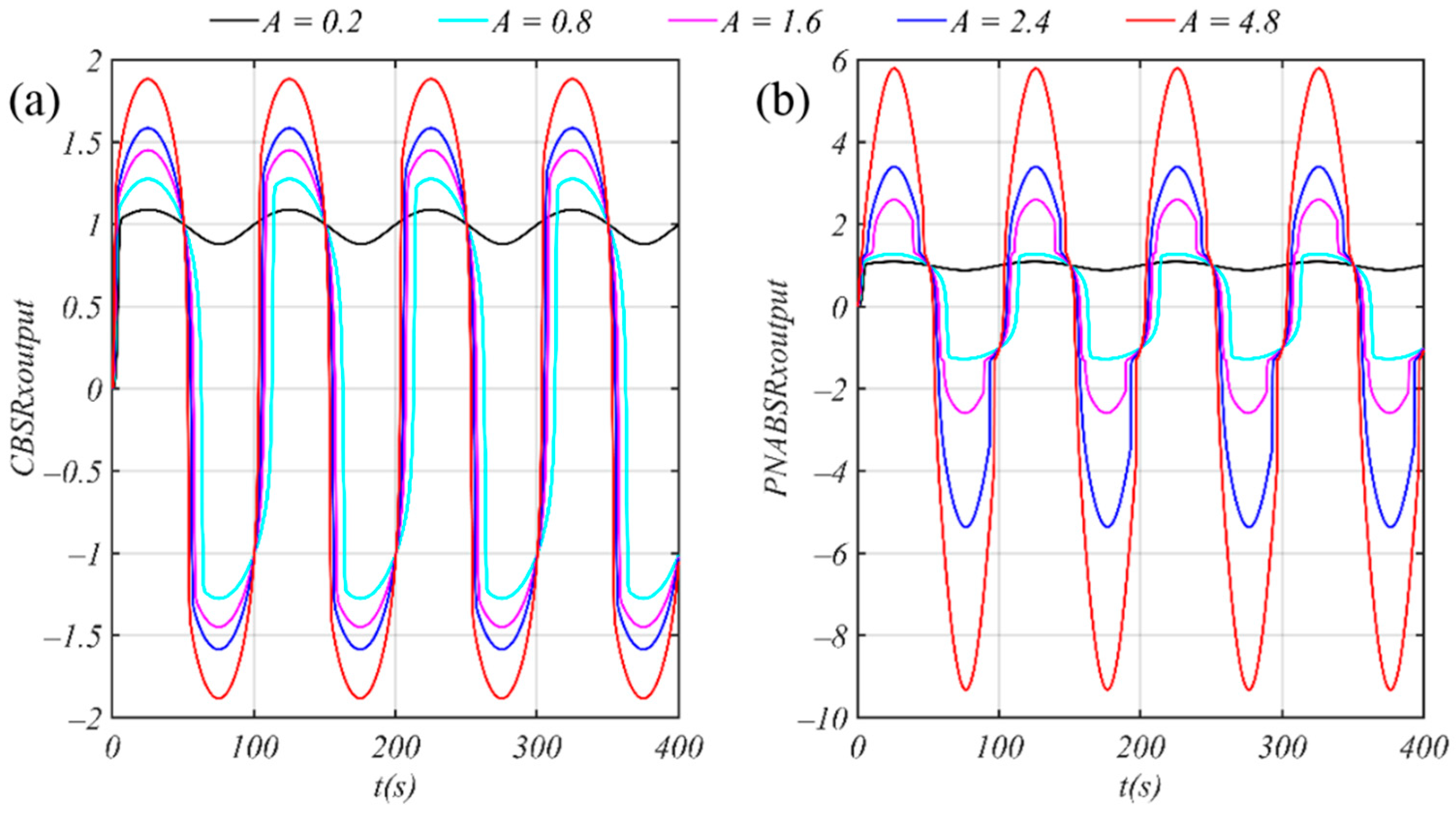
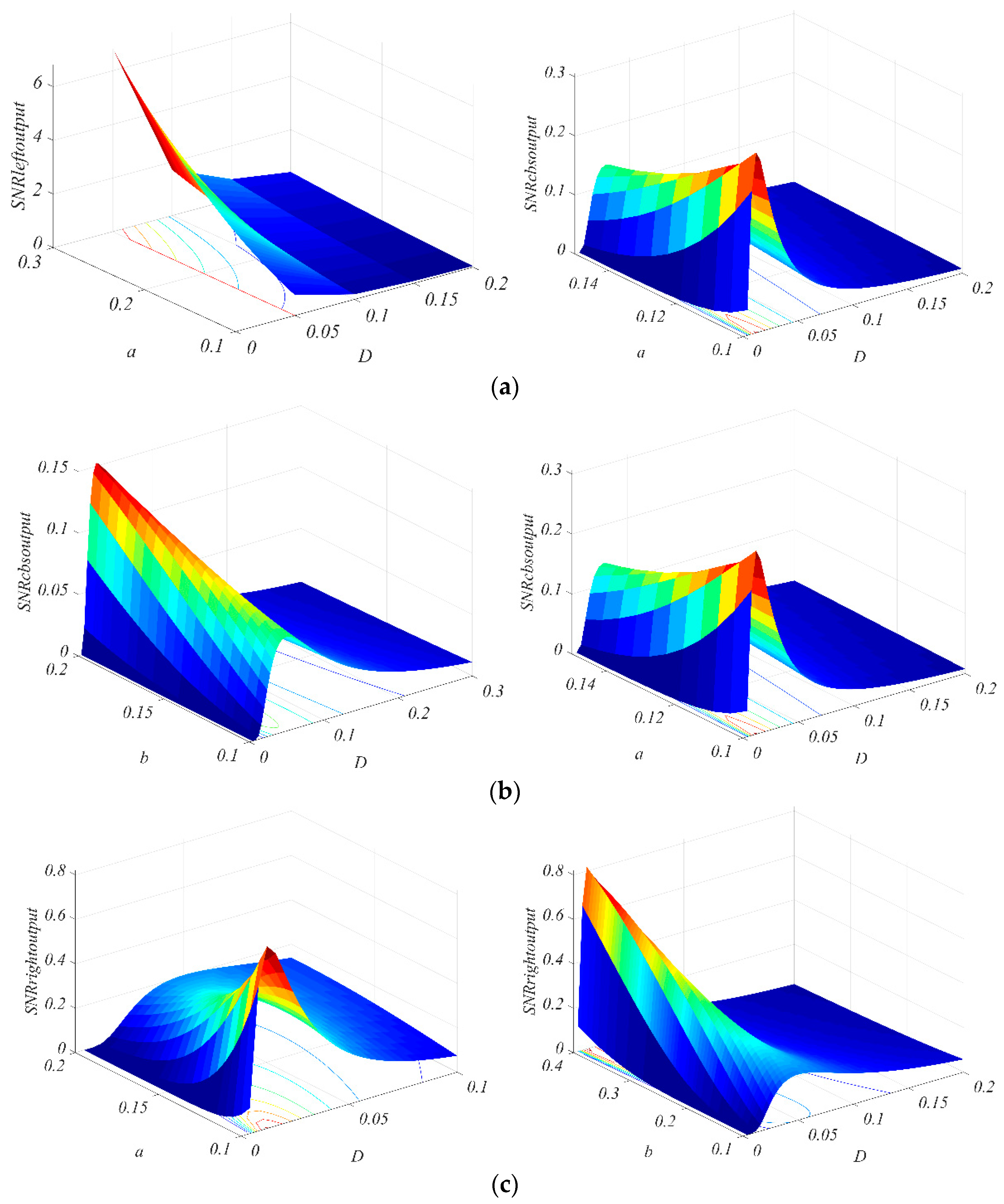
2.2. PNABSR Model and Its Performances

In order to overcome the shortcomings of the output saturation in the traditional stochastic resonance model, a new PNABSR model, different from the previous segmented model, was proposed. This system is composed of a monostable system and a structured asymmetric bistable system. The potential function of the new model is as follows:
U ( x ) = { a 2 4 b ( x + c c a / b ) , x < a / b 1 2 a x 2 + 1 4 b x 4 , a / b x a / b 1 2 a ( x a / b ) 2 a 2 4 b , x > a / b
where a > 0 ,   b > 0 ,   and   c > a / b (parameters a, b, and c are all constants). The first derivative of the potential function of the PNABSR method can be written as:
d U ( x ) d x = { a 2 4 b ( c a / b ) , x < a / b a x + b x 3 , a / b x a / b x a a / b , x > a / b
Figure 2 shows the potential function of the PNABSR and CBSR models as well as their barrier depth and potential wall height. The height that hinders particle movement is Δ U = a 2 / 4 b . From the potential function of the traditional stochastic resonance, as the output signal increases, the potential wall rapidly becomes steeper at that time. Hence, the potential energy cannot have a large impact on the output signal.
From Figure 2, it can be concluded that a small change in signal x can be observed. In the absence of noise, the particle will be in either of the two potential wells, and the system is not strong enough for the particles to move from one potential well to the other. By increasing the driving force and the noise, the particles can cross the peak of the barrier, resulting in a large-scale continuous transition between the 2D potential wells and the stochastic resonance phenomenon.
After setting a = 1 ,   b = 1 ,   and   c = 2 a / b , the fourth-order Runge–Kutta method was used for numerical simulation. Figure 3 shows a comparison of the output signals for the CBSR and PNABSR models. It can be observed that saturation exists in the CBSR model. However, the PNABSR method breaks through the limitations of saturation. When the amplitude of the input signal is A = 0.2, then the value of x o u t p u t is always greater than zero. It can be determined that the particles are always active on the right half of the model. When A increases, the particles move from the right well to the left well. As A changes, the output signal of PNABSR changes significantly. As shown in Figure 3, in order to expand the verification range of the saturation characteristics, the range of A is increased from 0.2 to 4.8. It can be clearly observed that the output signal of the PNABSR model has a faster growth rate and greater amplitude than that of the CBSR method. The results show that the proposed segmented asymmetric bistable system has a certain effect on suppressing the output saturation.
After setting parameter b = 1, parameter a varies from 1 to 1.8. Figure 4a,b show the change in the potential function in the PNABSR model. As the value of parameter a increases, the depth of the potential well of the PNABSR system increases, and the width of the potential well expands.
The PNABSR model is a two-state system with occupation probabilities. The signal power spectrum can be obtained by means of the following expression [11]:
S ( w ) = S N ( w ) + S s ( w )
where S N ( w ) and S s ( w ) represent the power spectrum of noise and the input signal, respectively.
S s ( w ) = π 2 ( A x m D ) 2 4 K 2 4 K 2 + w 0 2 [ δ ( w w 0 ) + δ ( w + w 0 ) ]
S N ( w ) = [ 1 1 2 ( A x m D ) 2 4 K 2 4 K 2 + w 0 2 ] 4 x m 2 4 K 2 + w 0 2
where x m = ± a / b and w 0 = 2 π f 0 ; w is the frequency of the signal; and K is the Kramers rate.
The SNR of a bistable system is defined as the ratio of the input signal power and the average power of the noise spectrum at w = w 0 , which can be obtained as follows [11]:
S N R o u t p u t = S s ( w ) d w S N ( w 0 )
Then, the theoretical value of the output of the S N R P N A B S R can be regarded as including three parts:
S N R l e f t = π ( A x m D ) 2 K = π a 3 A 2 4 D 2 b 2 a / b ( c a / b ) e a 2 4 b D
S N R m i d d l e = π 2 ( A x m D ) 2 K C B S R
S N R r i g h t = π 2 ( A x m D ) 2 K [ 1 1 2 ( A x m D ) 2 4 K 2 4 K 2 + w 0 2 ] 1 π 2 ( A x m D ) 2 K
where A 1 ,   D 1 (parameters A and D are constants), c = ( 2 / 2 + 1 ) a / b , and K C B S R = a 2 π e x p ( a 2 4 b D ) [19,20].
The S N R PNABSR can be obtained through numerical integration. The intermediate potential function is the same as the CBSR model, which is S N R c b s .
Figure 5 shows the change in the SNR of the PNASBR model under different parameters. An increase in the value of b will affect the SNR of the left and right potential functions. It can be seen that the S N R PNABSR changes as the noise intensity increases, rather than being monotonic, which indicates the appearance of stochastic resonance.
Figure 6a shows the change in the SNR’s theoretical value as the left potential function changes with parameters a and b, indicating that the SNR is larger when the parameter value is smaller. As shown in Figure 6b,c, when the noise intensity D increases, the SNR on the middle and right side of the PNABSR model first increases and then decreases, and there is a maximum value. Similarly, it can also be observed that the output S N R P N A B S R curve changes nonlinearly. This change in the SNR is due to the emergence of stochastic resonance. Under the appropriate noise intensity, stochastic resonance will lead to changes in the signal energy.

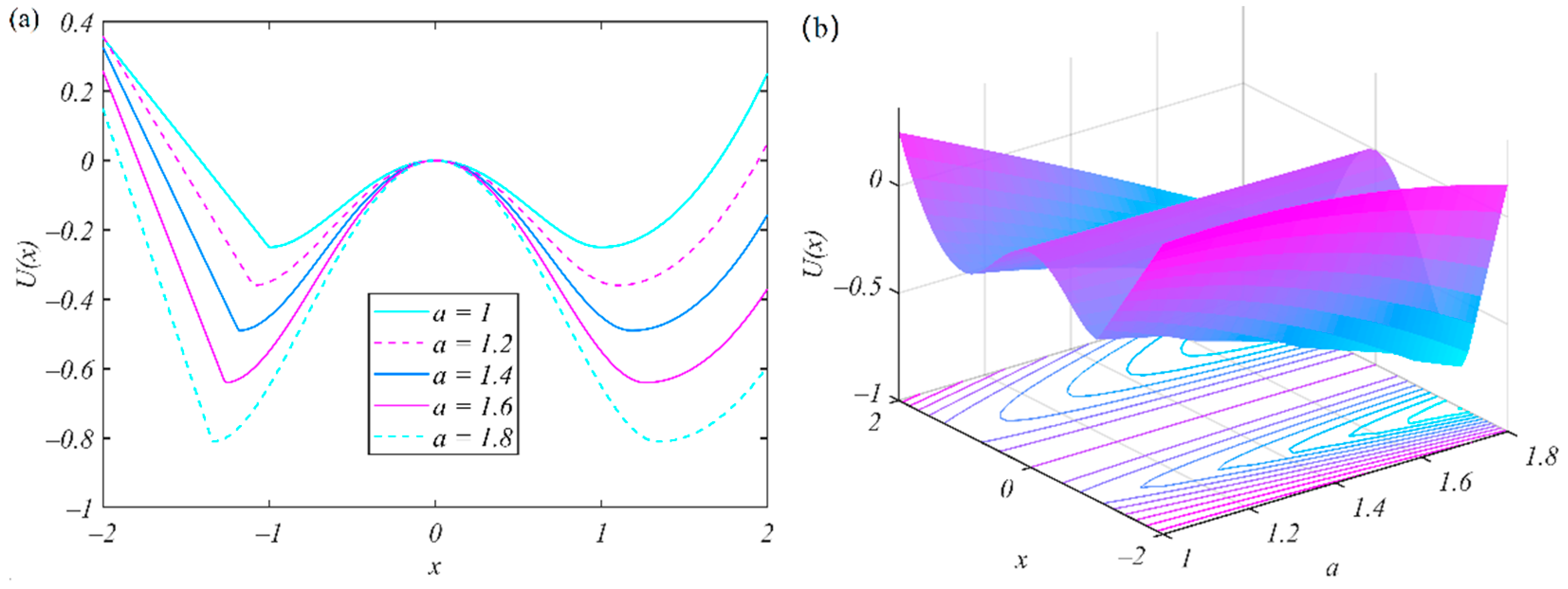
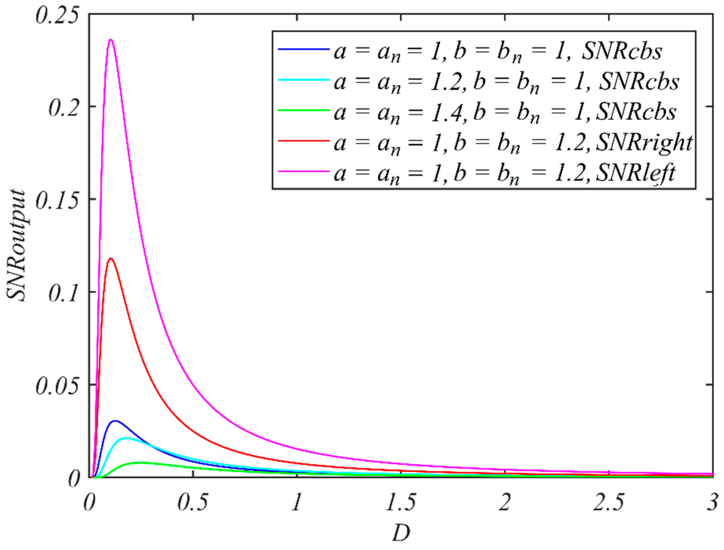
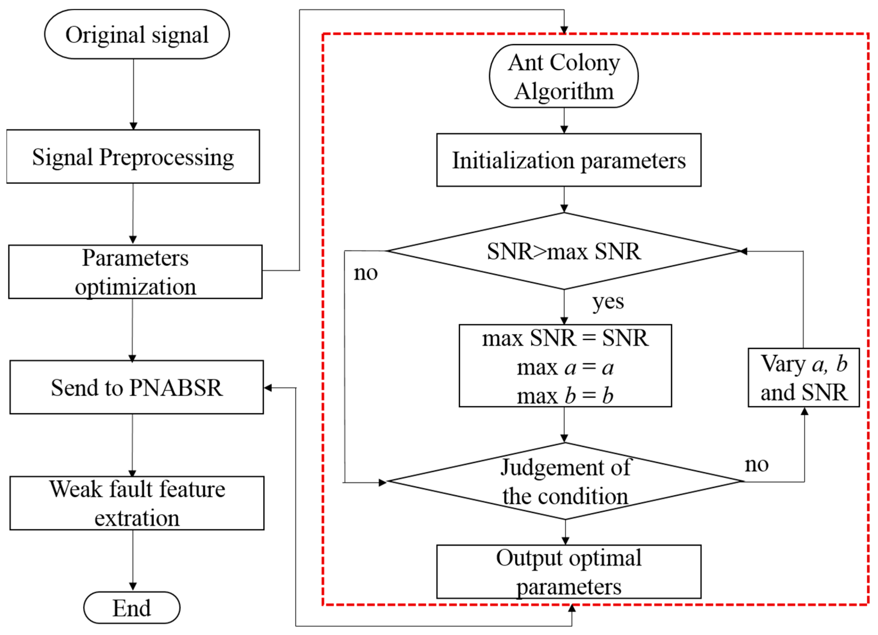
2.3. Optimization of PNABSR Parameters

The performance of the PNABSR model depends on the selection of its parameters. In this paper, the adaptive ant colony intelligent algorithm is used to optimize the parameters for the PNABSR model. The objective function is defined as follows [21]:
S N R = 10 l o g 10 ( H d i = 1 N / 2 H i H d )
where H d is the power of the drive frequency, and i = 1 N / 2 H i H d represents the total noise power.
A higher output SNR means that the PNABSR model has a stronger weak fault feature extraction ability. The detailed process is shown in Figure 7.
Firstly, the original signal is preprocessed. The signal is compressed using frequency shift and scaling, and the compression ratio is set to 2400. Secondly, the signal is input into the PNABSR parameter optimization program by the adaptive ant colony intelligent algorithm. The number of ants is set to 100, and the pheromone evaporation coefficient Rho is 0.9. The maximum number of iterations is 5. The optimization range of the system parameters is set from 0 to 10. The maximum output SNR of the PNABSR model is set as the objective function in the adaptive optimization ant colony algorithm. If the SNR difference between the two outputs is less than 0.1, then the optimal parameters of the PNABSR model can be obtained. Then, the optimized parameters are sent to the PNABSR model. Finally, the signals are processed by PNABSR, and the weak fault features are extracted.

3. Analysis and Discussion

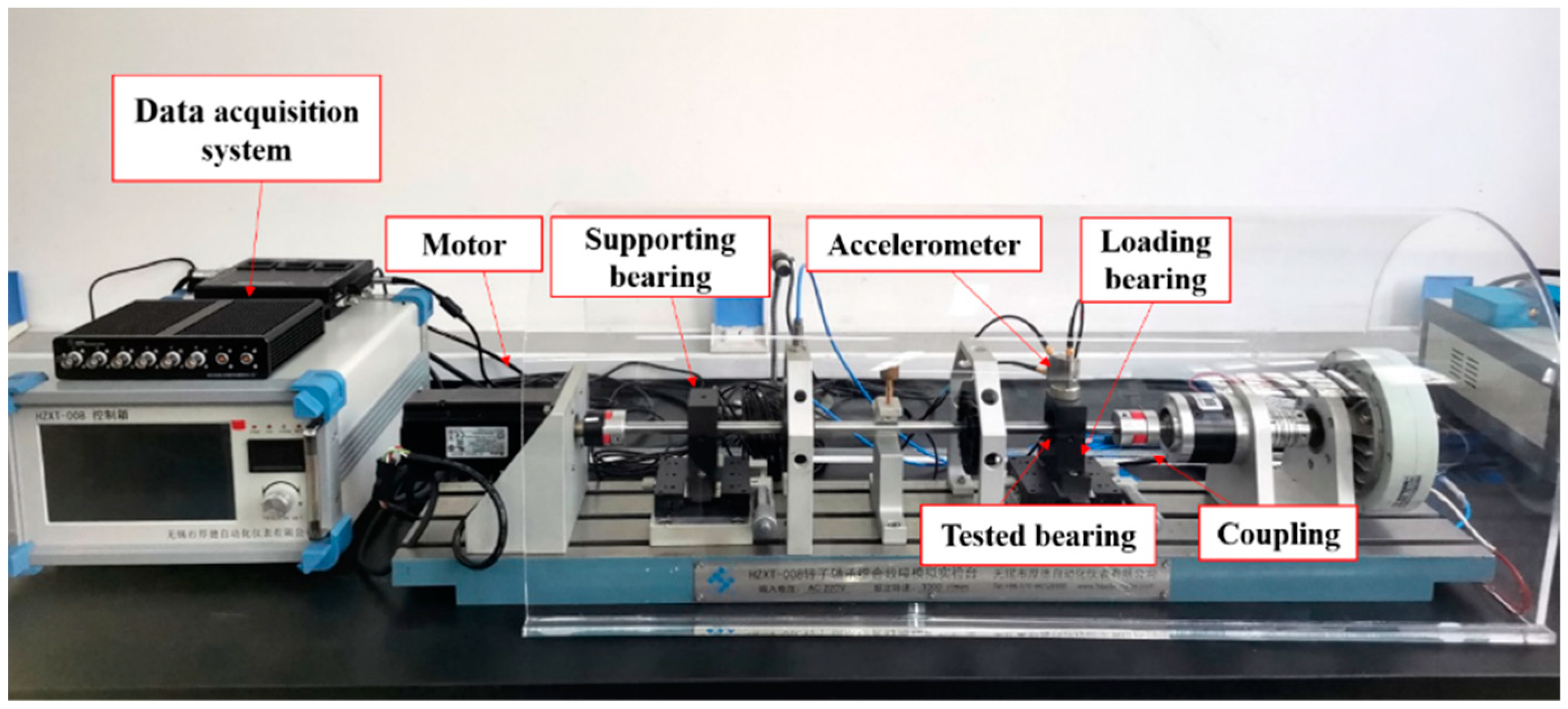
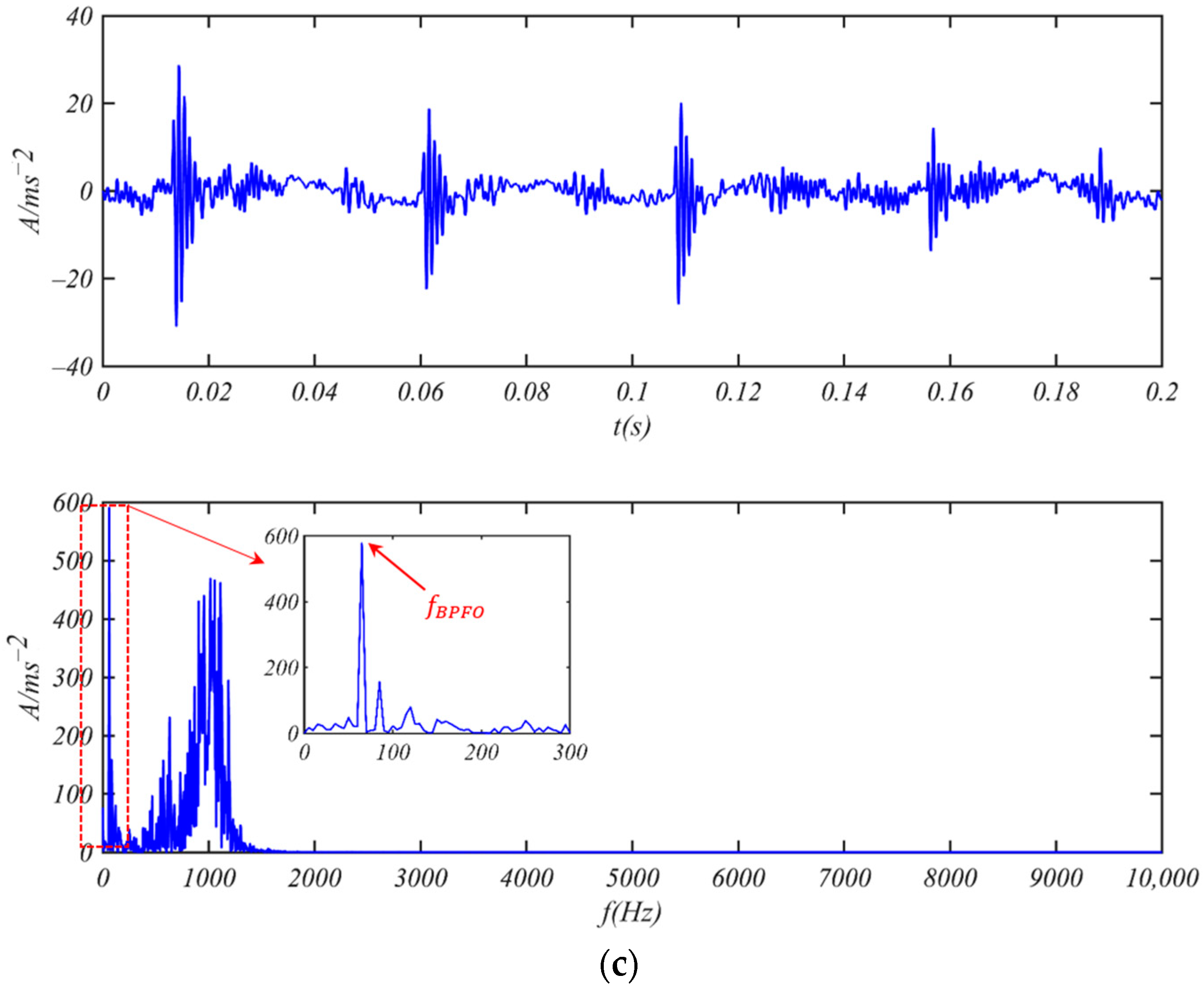
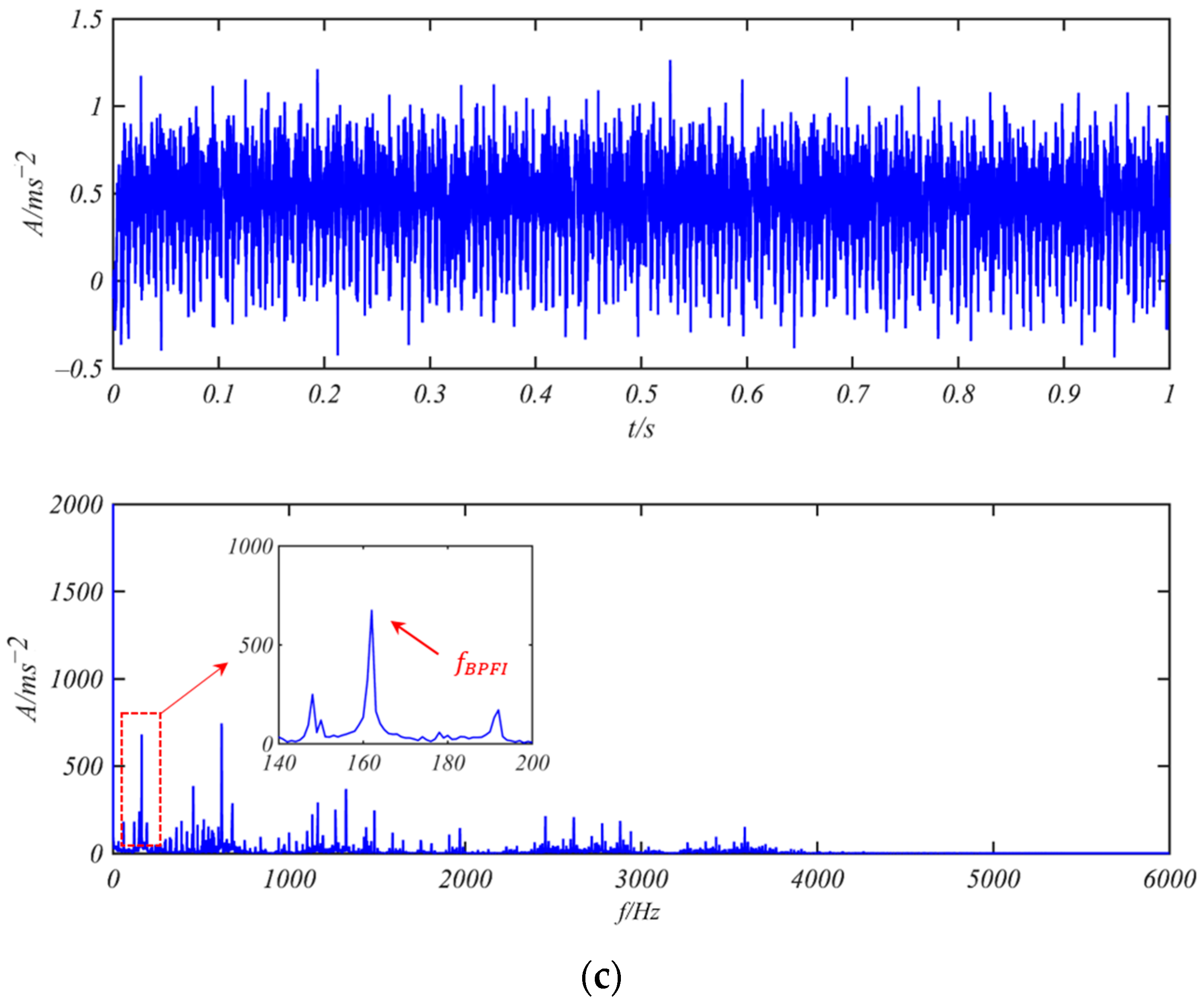
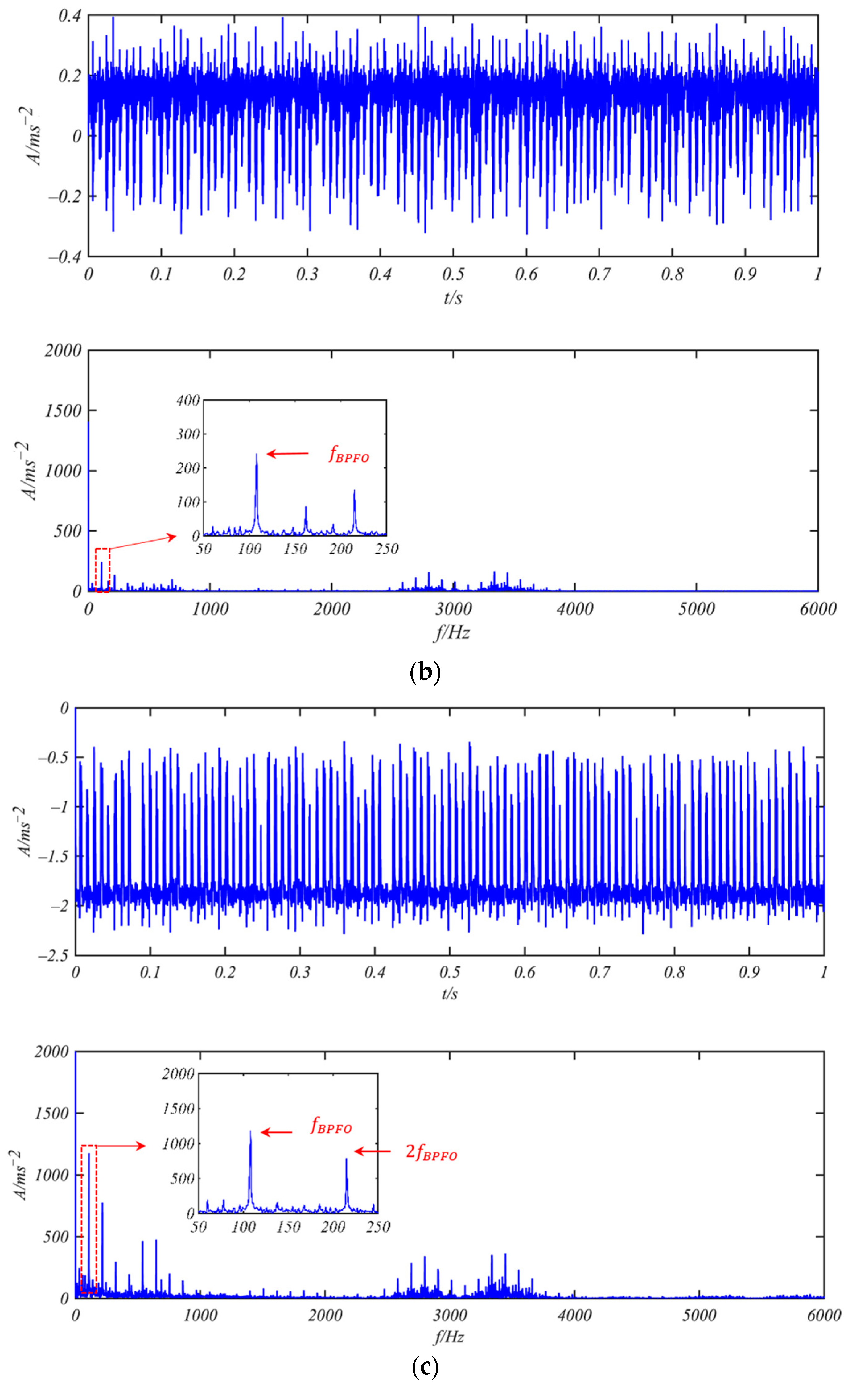
3.1. Fault Detection of Bearing SKF 6205-2RS

To verify the reliability of the PNABSR model, 6205-2RS bearings with an inner ring fault and outer ring fault were used [22]. Table 1 shows the parameters of the deep groove 6205-2RS ball bearings.
The test parameters were set as follows: sampling frequency fs = 12,000 Hz; rotating = 1750 r/min. The fault frequencies of the inner and outer ring were set to f BPFI = 162 Hz and f BPFO = 107 Hz. The intensity of the added noise was 0.35.
(1)
Bearing 6205-2RS JEM SKF with Weak Inner Ring Fault
Figure 8a provides the original signal data with the inner ring fault, and it is obvious that the fault characteristic frequency cannot be found. As shown in Figure 8b,c, the inner ring fault can be diagnosed by both the CBSR and PNABSR models. In addition, in Figure 8b,c, the peaks of the power spectrum between 1000 Hz and 2500 Hz are obviously reduced. The occurrence of this phenomenon can be understood as the transfer of high-frequency energy to low-frequency energy. The signal-to-noise ratios obtained by the CBSR and PNABSR models are −23.74dB and −16.35 dB. The optimized parameters of the CBSR and PNABSR models are a = 0.2 and b = 0.8 as well as a = 0.2 and b = 0.6, respectively. Compared to the results of Figure 8b,c, the value of the power spectrum processed by the PNABSR model is much greater than the value of the power spectrum processed by the CBSR model. The weak inner ring fault of the bearing can be identified clearly by the PNABSR model.
(2)
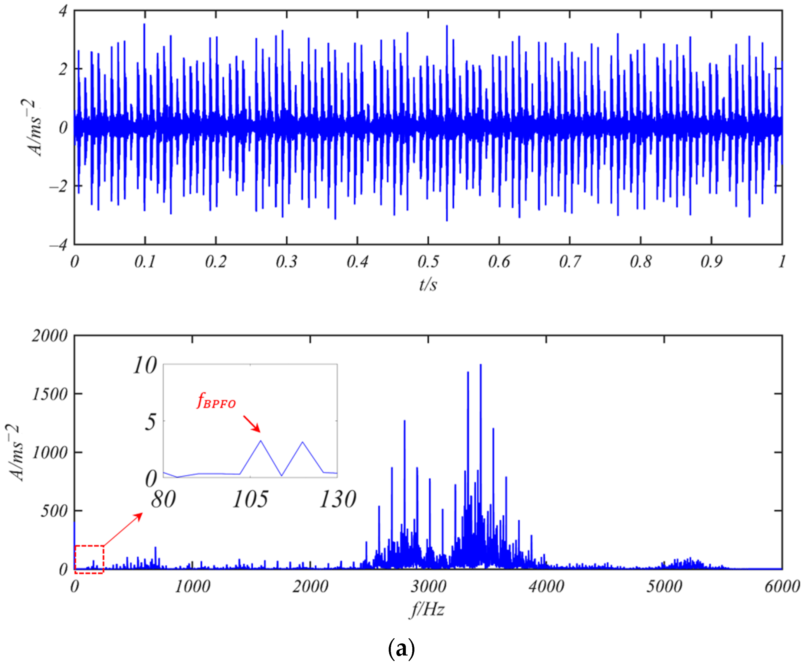
Bearing 6205-2RS JEM SKF with Weak Outer Ring Fault
Figure 9a provides the original signal with the outer ring fault. Figure 9b,c show the signals processed by the CBSR and PNABSR models. It was found that the power spectrum peaks at the fault frequency from the PNABSR model are more prominent than those of the CBSR model. Figure 9c shows that the double frequency of the outer ring fault is also identified. The optimized parameters of the CBSR system and the PNABSR system are a = 0.5 and b = 0.7 as well as a = 0.4 and b = 0.6, respectively. The signal-to-noise ratios obtained by the CBSR and PNABSR models are −25.32 dB and −13.56 dB, respectively. A weak inner ring fault of the bearing can be clearly identified by the PNABSR model.

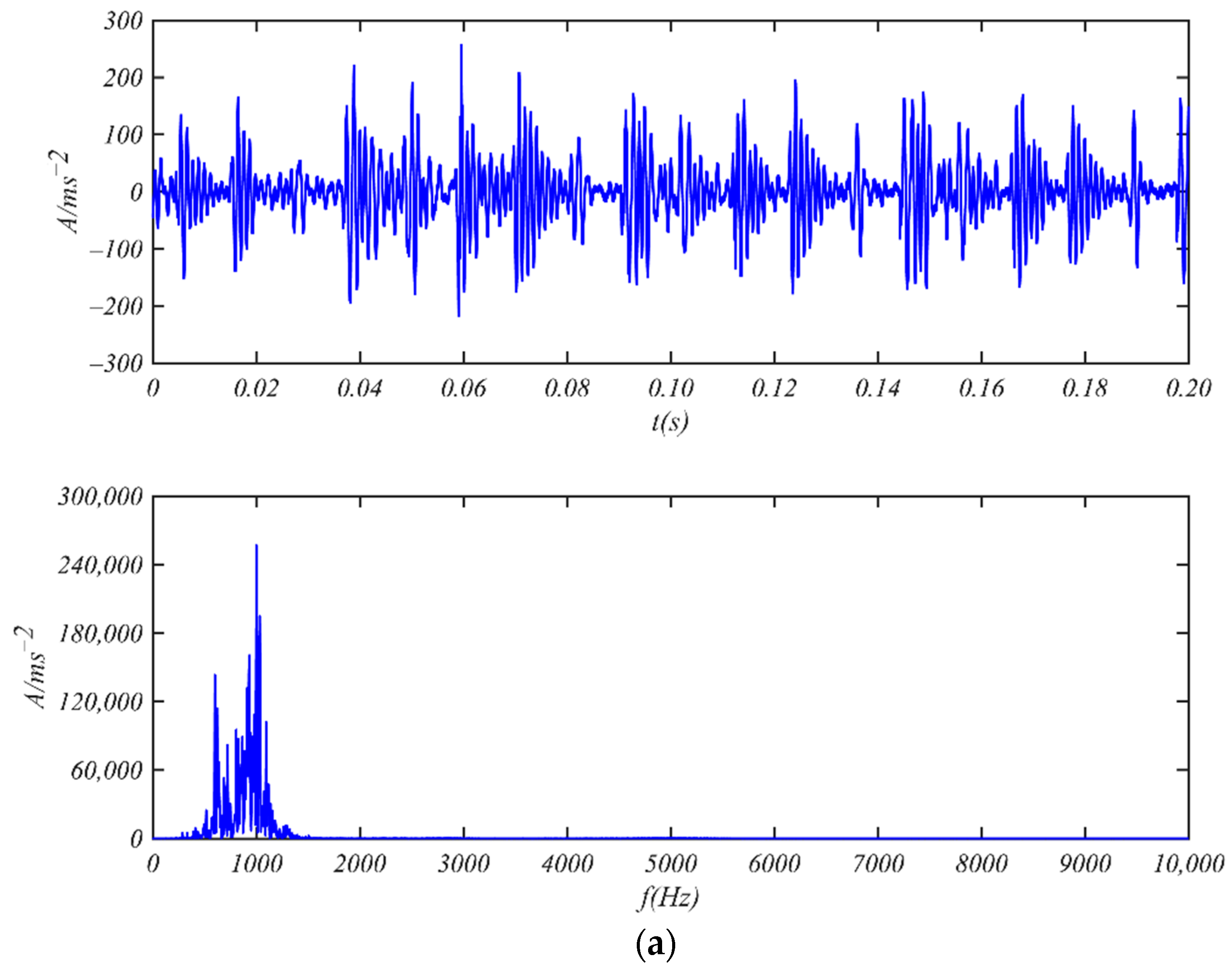
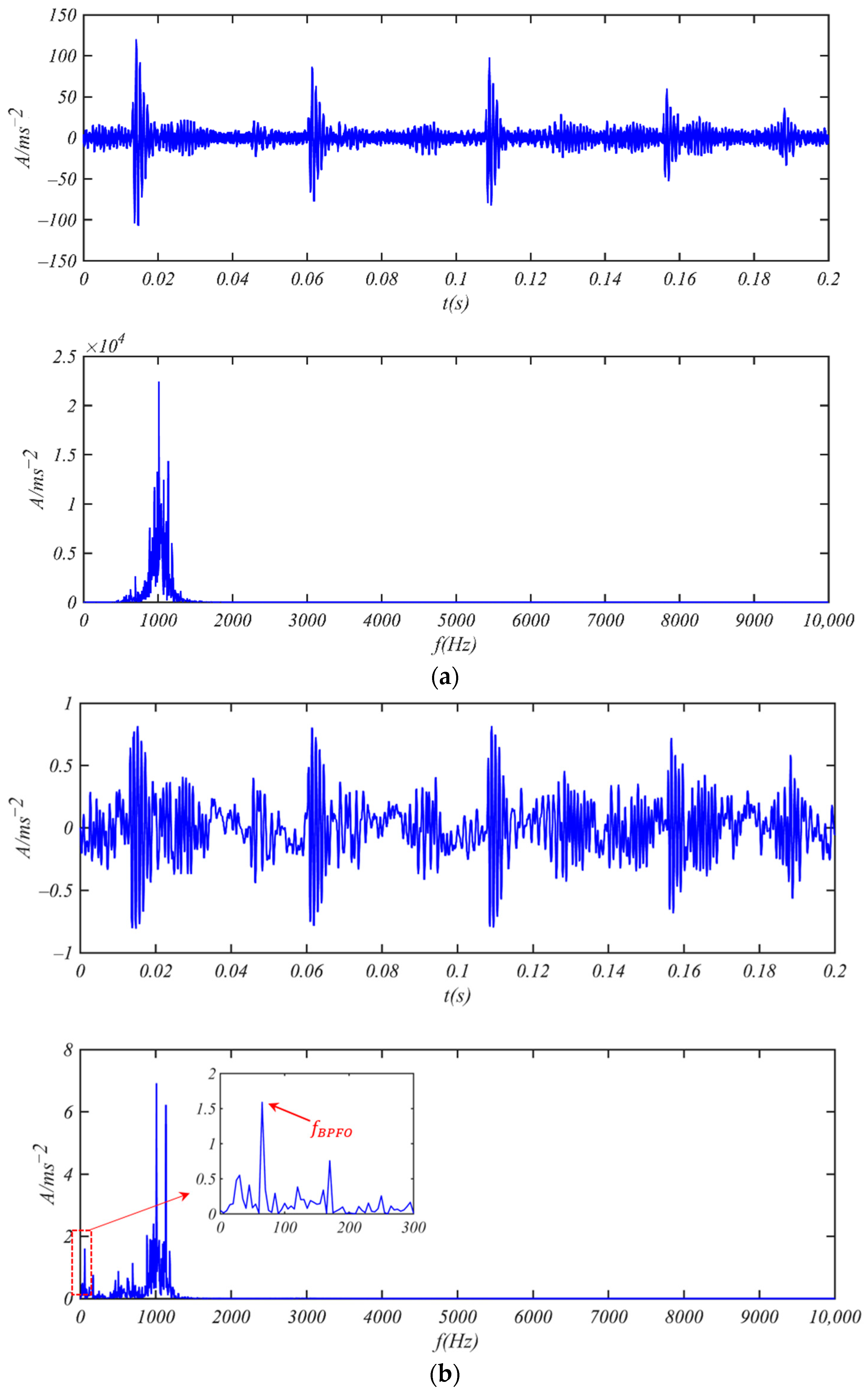
3.2. Weak Fault Detection Experiments of Bearing 6200-NR NSK

Verification experiments were carried out using the bearing test bench under different speeds and loads. The vibration signals were sampled by acceleration sensors, as shown in Figure 10. The bearing parameters are shown in Table 2. The sample frequency was set as 20 kHz, and the rotational speed was set as 1300 r/min. Here, f B P F O = 66.535   Hz and f B P F I = 106.799   Hz ; D = 0.01, and the re-scaling ratio was set as R = 4000.
(1)
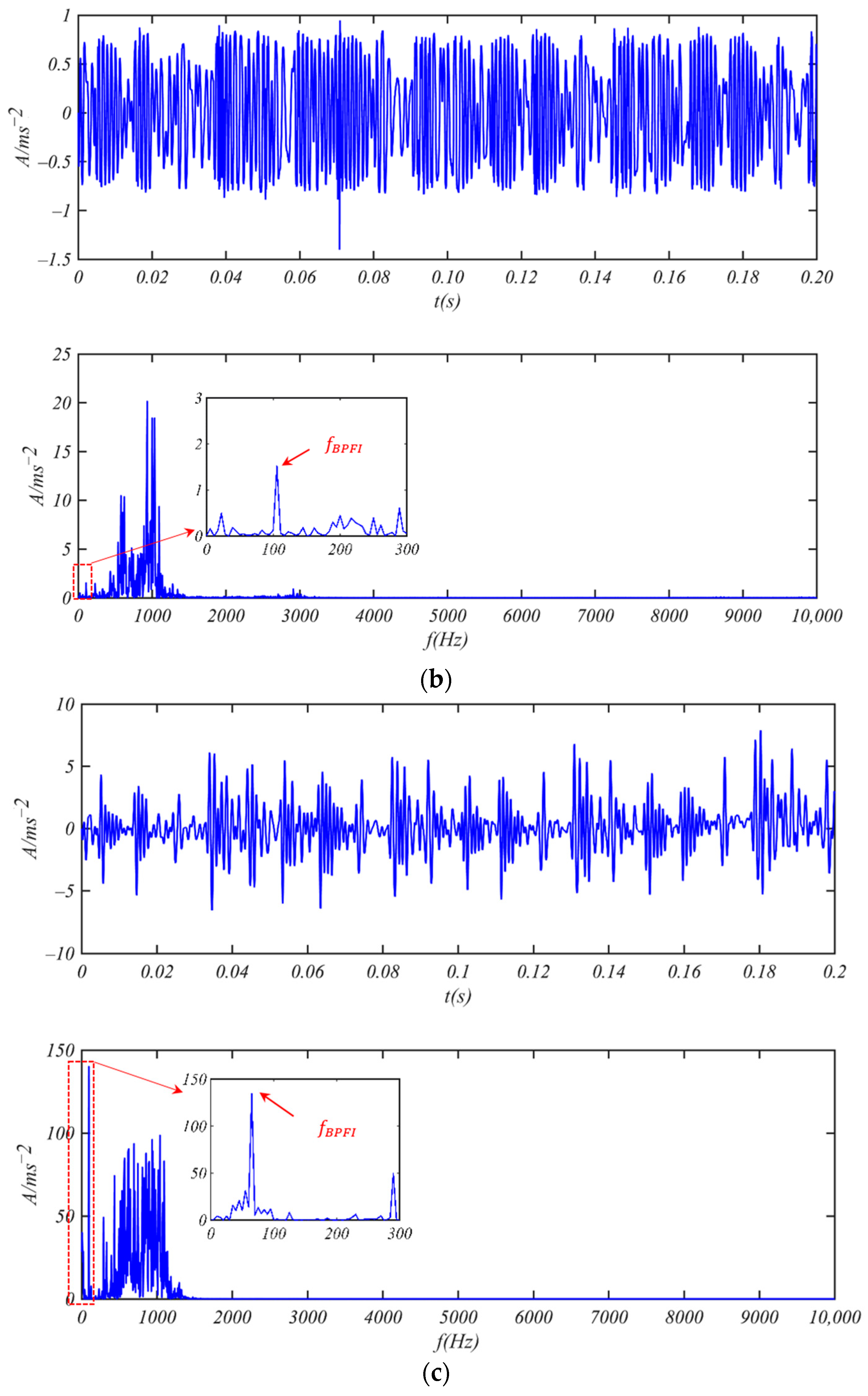
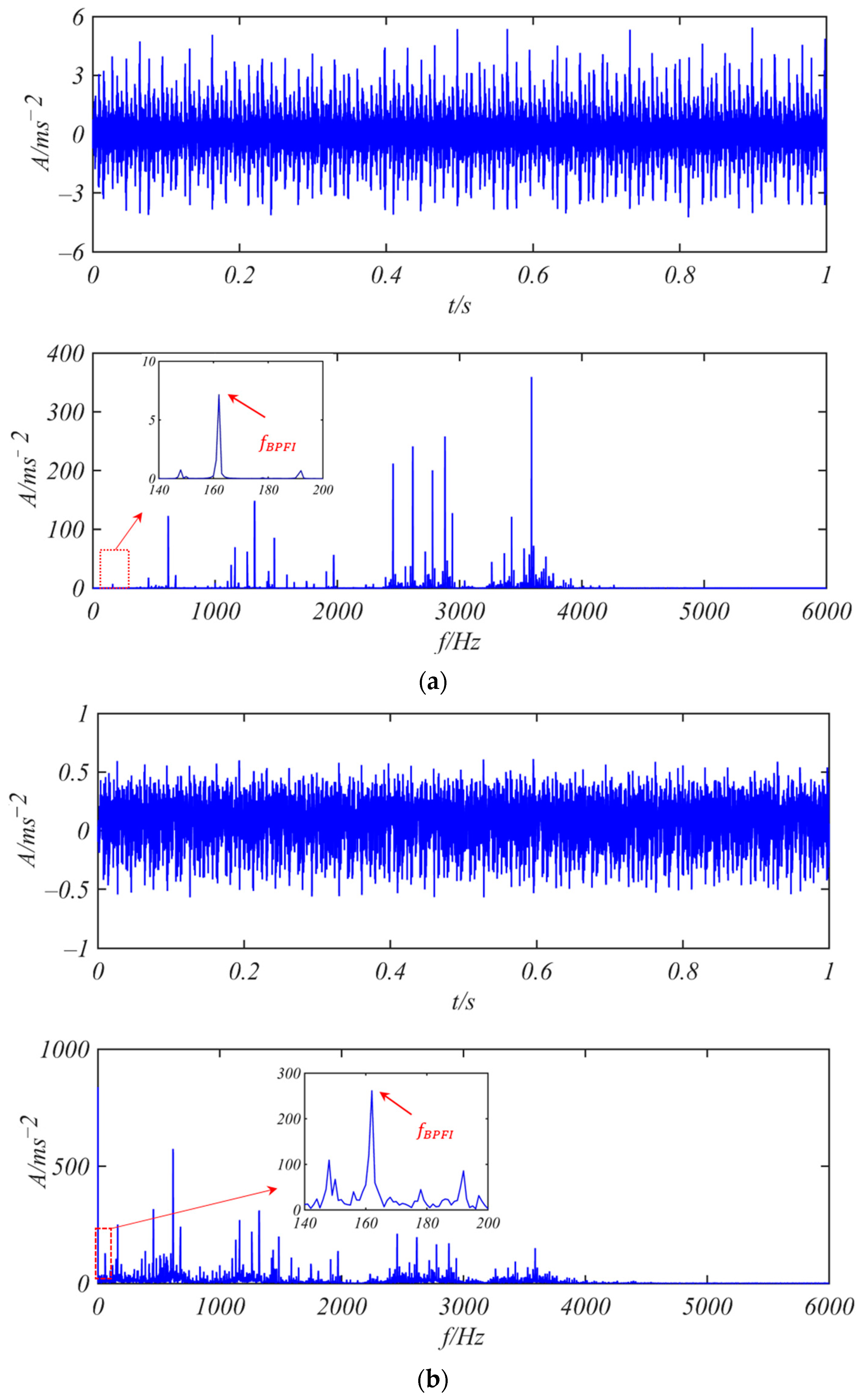
6200-NR NSK Bearing with Weak Inner Ring Fault
Figure 11 compares the 6200-NR bearings with the inner ring fault processed by the different models. In Figure 11a, the fault characteristic frequency cannot be identified, and the weak fault signal is submerged in strong background noise. From Figure 11b,c, the peak can be observed by the PNABSR method and is more prominent, and the peak value is about 30 times that of the CBSR method. The optimized parameters of the CBSR system and the PNABSR system are a = 0.03 and b = 0.8 as well as a = 0.04 and b = 0.6, respectively. The output SNR values of the CBSR and PNABSR models are −25.13 dB and −10.86 dB, respectively. It can be seen that the PNABSR model is more suitable for weak fault extraction because it can amplify amplitude and improve the SNR of the weak fault.
(2)
6200-NR NSK Bearing with Weak Outer Ring Fault
Figure 12 provides a comparison of the 6200-NR bearings with an outer ring fault processed by the different models. As shown in Figure 12a, the frequency components are concentrated between 800 Hz and 1200 Hz. In Figure 12b,c, a power spectrum peak at f = f B P F O can be observed. The fault diagnosis is more obvious in Figure 12c. The SNR outputs of the CBSR and PNABSR models are −27.29 dB and −13.05 dB, respectively. The optimized parameters of the CBSR system and PNABSR system are a = 0.04 and b = 0.5 as well as a = 0.08 and b = 0.4, respectively. This verifies the effectiveness of the PNABSR model, which is more suitable for weak fault extraction.

4. Conclusions

This paper proposes a new PNASBR model that is able to avoid output saturation by establishing a piecewise asymmetric bistable model that is more conducive to weak fault signal extraction than the traditional CBSR model. Through theoretical analysis and experimental verification, the following conclusions were obtained:
  • In this paper, a coupled piecewise nonlinear asymmetric bistable stochastic resonance system is proposed, and the signal-to-noise ratio equation is derived.
  • Using the ant colony intelligent algorithm to optimize parameters a and b, the signal-to-noise ratio of the PNABSR model can be 45% higher than that of the traditional CBSR model. It is easier for the PNABSR model to induce stochastic resonance.
  • The test results show that the PNABSR model can observe the fault feature more clearly in practical applications. By comparing the experimental results of the CBSR and PNABSR models, it was found that the PNABSR system has outstanding advantages in terms of the amplitude amplification of weak fault characteristics and in improving the signal-to-noise ratio.
  • The PNABSR model is suitable for weak fault extraction, especially under the conditions of strong background noise. Because the effectiveness of this model depends on parameter optimization, there is a certain time delay for real-time fault diagnosis.
  • The extraction of the weak fault features is the first step of fault diagnosis. However, fault classification, fault degree evaluation, and prediction are also very important for the operation and maintenance of engineering equipment. We intend to discuss these problems in our future work.

Author Contributions

Conceptualization, L.C. and W.X.; methodology, W.X.; software, L.C.; validation, L.C. All authors have read and agreed to the published version of the manuscript.

Funding

This work was financially supported by the Shanghai Natural Science Foundation (No. 20ZR1421000) and the National Natural Science Foundation of China (No. 51675323).

Institutional Review Board Statement

Not applicable.

Informed Consent Statement

Not applicable.

Data Availability Statement

The data that support the findings of this study are available from the corresponding author upon reasonable request.

Conflicts of Interest

The authors declare no conflict of interest.

References

  1. Benzi, R.; Sutera, A.; Vulpiani, A. The mechanism of stochastic resonance. J. Phys. A Math. Gen. 1981, 14, 453. [Google Scholar] [CrossRef]
  2. Chen, H.; Varshney, P.K.; Kay, S.M.; Michels, J.H. Theory of the Stochastic Resonance Effect in Signal Detection: Part I-Fixed Detectors. IEEE Trans. Signal Process. 2007, 55, 3172–3184. [Google Scholar] [CrossRef]
  3. Chen, H.; Varshney, L.R.; Varshney, P.K. Noise-enhanced information systems. Proc. IEEE 2014, 102, 1607–1621. [Google Scholar] [CrossRef] [Green Version]
  4. Fauve, S.; Heslot, F. Stochastic resonance in a bistable system. Phys. Lett. A 1983, 97, 5–7. [Google Scholar] [CrossRef]
  5. McNamara, B.; Wiesenfeld, K. Theory of stochastic resonance. Phys. Rev. Let. 1988, 60, 2626–2629. [Google Scholar] [CrossRef]
  6. Kang, Y.M.; Wang, M.; Xie, Y. Stochastic resonance in coupled weakly-damped bistable oscillators subjected to additive and multiplicative noises. Acta Mech. Sin. 2012, 28, 505–510. [Google Scholar] [CrossRef]
  7. Randall, R.B.; Antoni, J. Rolling element bearing diagnostics-A tutorial. Mech. Syst. Signal Process. 2011, 25, 485–520. [Google Scholar] [CrossRef]
  8. Antoni, J.; Randall, R.B. Unsupervised noise cancellation for vibration signals: Part II-a novel frequency-domain algorithm. Mech. Syst. Signal Process. 2004, 18, 103–117. [Google Scholar] [CrossRef]
  9. Wang, L.; Zhao, W. A new piecewise-linear stochastic resonance model. In Proceedings of the 2009 IEEE International Conference on Systems, Man and Cybernetics, San Antonio, TX, USA, 11–14 October 2009; pp. 5209–5214. [Google Scholar]
  10. Qiao, Z.; Lei, Y.; Lin, J.; Jia, F. An adaptive unsaturated bistable stochastic resonance method and its application in mechanical fault diagnosis. Mech. Syst. Signal Process. 2017, 84, 731–746. [Google Scholar] [CrossRef]
  11. Zhang, G.; Hu, D.; Zhang, T. Stochastic resonance in unsaturated piecewise nonlinear bistable system under multiplicative and additive noise for bearing fault diagnosis. IEEE Access 2019, 7, 58435–58448. [Google Scholar] [CrossRef]
  12. Tang, J.; Shi, B.; Bao, H.; Li, Z. A new method for weak fault feature extraction based on piecewise mixed stochastic resonance. Chin. J. Phys. 2020, 68, 87–99. [Google Scholar] [CrossRef]
  13. Zhao, S.; Shi, P.; Han, D. A novel mechanical fault signal feature extraction method based on unsaturated piecewise tri-stable stochastic resonance. Measurement 2021, 168, 108374. [Google Scholar] [CrossRef]
  14. Huang, X. Stochastic resonance in a piecewise bistable energy harvesting model driven by harmonic excitation and additive Gaussian white noise. Appl. Math. Model. 2021, 90, 505–526. [Google Scholar] [CrossRef]
  15. Xu, P.; Jin, Y. Stochastic resonance in an asymmetric tristable system driven by correlated noises. Appl. Math. Model. 2020, 77, 408–425. [Google Scholar] [CrossRef]
  16. Liu, X.; Liu, H.; Yang, J.; Litak, G.; Cheng, G.; Han, S. Improving the bearing fault diagnosis efficiency by the adaptive stochastic resonance in a new nonlinear system. Mech. Syst. Signal Process. 2017, 96, 58–76. [Google Scholar] [CrossRef]
  17. Leng, Y.G.; Leng, Y.S.; Wang, T.Y.; Guo, Y. Numerical analysis and engineering application of large parameter stochastic resonance. J. Sound Vib. 2006, 292, 788–801. [Google Scholar] [CrossRef]
  18. Cheng, W.; Xu, X.; Ding, Y.; Sun, K.; Li, Q.; Dong, L. An adaptive smooth unsaturated bistable stochastic resonance system and its application in rolling bearing fault diagnosis. Chin. J. Phys. 2020, 65, 629–641. [Google Scholar] [CrossRef]
  19. Casado-Pascual, J.; Gómez-Ordóñez, J.; Morillo, M. Stochastic resonance: Theory and numerics. Chaos Interdiscip. J. Nonlinear Sci. 2005, 15, 026115. [Google Scholar] [CrossRef]
  20. Di Paola, M.; Sofi, A. Approximate solution of the Fokker–Planck–Kolmogorov equation. Probabilistic Eng. Mech. 2002, 17, 369–384. [Google Scholar] [CrossRef]
  21. Wang, J.; He, Q.; Kong, F. An improved multiscale noise tuning of stochastic resonance for identifying multiple transient faults in rolling element bearings. J. Sound Vib. 2014, 333, 7401–7421. [Google Scholar] [CrossRef]
  22. Li, J.; Zhang, J.; Li, M.; Zhang, Y. A novel adaptive stochastic resonance method based on coupled bistable systems and its application in rolling bearing fault diagnosis. Mech. Syst. Signal Process. 2019, 114, 128–145. [Google Scholar] [CrossRef]
Figure 1. Effect of parameters of CBSR model on saturation phenomenon.
Machines 10 00373 g001
Figure 2. Potential function of PNABSR and CBSR models.
Machines 10 00373 g002
Figure 3. Comparison of output signals of CBSR and PNABSR models: (a) CBSR; (b) PNABSR. (D = 0, f 0 = 0.01 Hz, f s = 10 Hz).
Machines 10 00373 g003
Figure 4. When b = 1, PNABSR’s potential function changes with parameters. (a) Potential function changes with a; (b) Potential function changes with a and x.
Machines 10 00373 g004
Figure 5. SNR of PNABSR changes with parameters a, b (A = 0.1,   f 0   = 0.01 Hz).
Machines 10 00373 g005
Figure 6. S N R P N A B S R changes with parameter a, b, and D. (a) The signal-to-noise ratio output of the left well:, b = 0.1, a = 0.1; (b) the signal-to-noise ratio output of the middle well: b = 0.1, a = 0.1; and (c) the signal-to-noise ratio output of the right well: b = 0.1, a = 0.1.
Machines 10 00373 g006
Figure 7. Optimization of PNABSR model parameters.
Machines 10 00373 g007
Figure 8. Comparison between different models to process bearing 6205 with inner ring fault: (a) origin time-domain signal and its spectrum; (b) time-domain signal and its spectrum processed by CBSR model; and (c) time-domain signal and its spectrum processed by PNABSR model.
Machines 10 00373 g008aMachines 10 00373 g008b
Figure 9. Comparison between different models to process bearing 6205 with outer ring fault: (a) origin time-domain waveform and spectrum; (b) time-domain signal and its spectrum processed by CBSR model; and (c) time-domain signal and its spectrum processed by PNABSR model.
Machines 10 00373 g009aMachines 10 00373 g009b
Figure 10. Bearing rotor fault test bench.
Machines 10 00373 g010
Figure 11. Comparison between different models to process bearing 6200 with inner ring fault: (a) origin time-domain waveform and spectrum; (b) time-domain waveform and spectrum processed by CBSR model; and (c) time-domain waveform and spectrum processed by PNABSR model.
Machines 10 00373 g011aMachines 10 00373 g011b
Figure 12. Comparison between different models to process bearing 6200 with outer ring fault: (a) origin time-domain waveform and spectrum; (b) time-domain waveform and spectrum processed by CBSR model; and (c) time-domain waveform and spectrum processed by PNABSR model.
Machines 10 00373 g012aMachines 10 00373 g012b
Table 1. Parameters of bearing 6205-2RS JEM SKF.
Inside Diameter
(mm)
Outside Diameter
(mm)
Width
(mm)
Ball
Diameter
(mm)
Pitch
Diameter
(mm)
Ball
Number
2552157.938399
Table 2. Parameters of bearing 6200-NR NSK.
Inside Diameter
(mm)
Outside Diameter
(mm)
Width
(mm)
Ball
Diameter
(mm)
Pitch
Diameter
(mm)
Ball
Number
103095.52010
Publisher’s Note: MDPI stays neutral with regard to jurisdictional claims in published maps and institutional affiliations.

