Anomaly Data Detection of Rolling Element Bearings Vibration Signal Based on Parameter Optimization Isolation Forest

Abstract

Anomaly data detection is not only an important part of the condition monitoring process of rolling element bearings, but also the premise of data cleaning, compensation and mining. Aiming at the abnormal data segment detection of the vibration signals of a rolling element bearing, this paper proposes an abnormal data detection model based on comprehensive features and parameter optimization isolation forest (CF-POIF), which can adaptively identify abnormal data segments. First, in order to extract the mutation feature of vibration signals more accurately, the concept of comprehensive feature is proposed, which integrates the time domain and wavelet packet energy features. Then, the particle swarm optimization (PSO) algorithm is used to optimize the rectangular window length and sub sample set capacity in the isolation forest for anomaly detection. Finally, three real cases concerning abnormal data are used to verify the effectiveness of the proposed method. The results demonstrate that the proposed method is able to detect missing data, drift data and external interference data effectively, and it has a higher $F_1$ score and accuracy compared to other methods.

1. Introduction

In the condition monitoring of rolling element bearings, the vibration data of rolling element bearings is usually collected by using sensors. Then, fault diagnosis is carried out in time domain, frequency domain or time-frequency domain based on these data [1,2]. Because the monitoring environment is often accompanied by strong vibration, sometimes there may be uncertain impacts on the normal operation of sensors. For example, in the actual vibration signal acquisition process, the vibration data in some time periods may be lost due to sensor failure, signal transmission or poor line contact [3,4]. 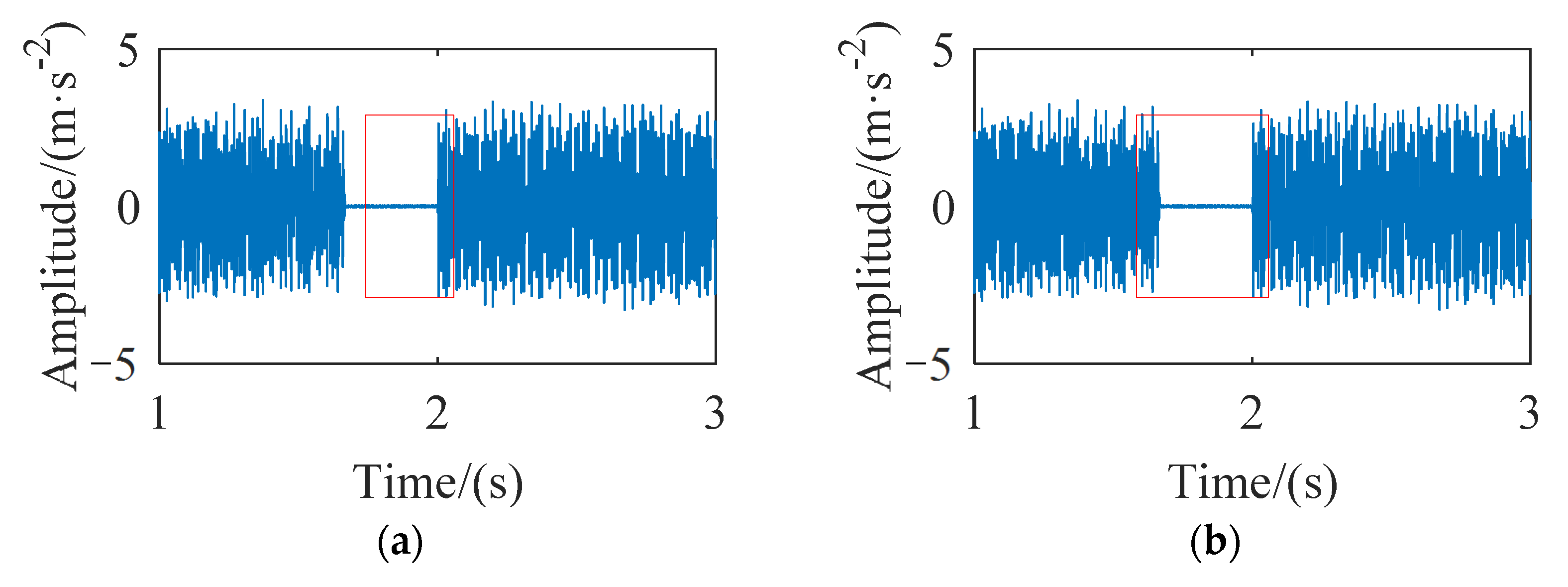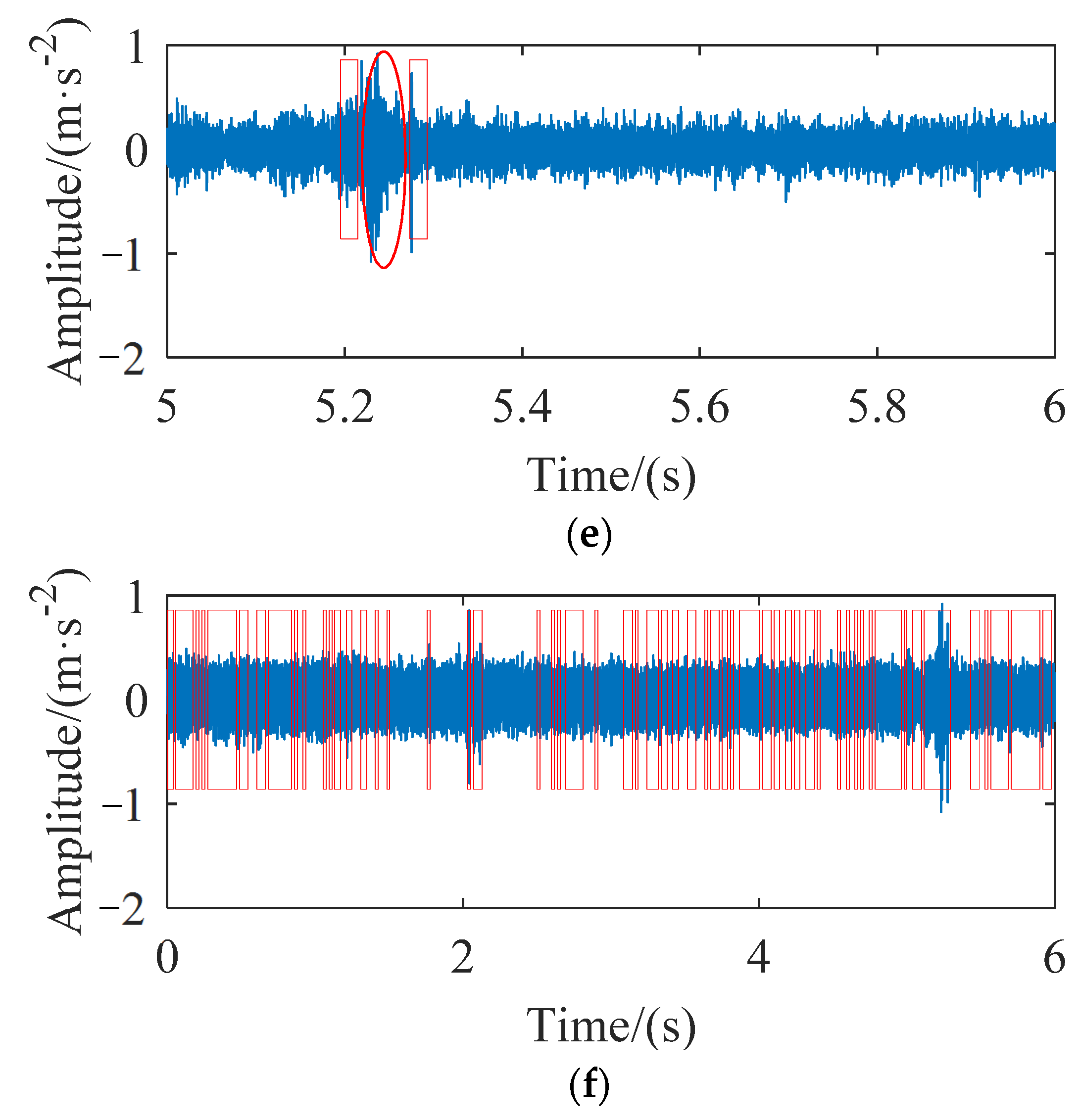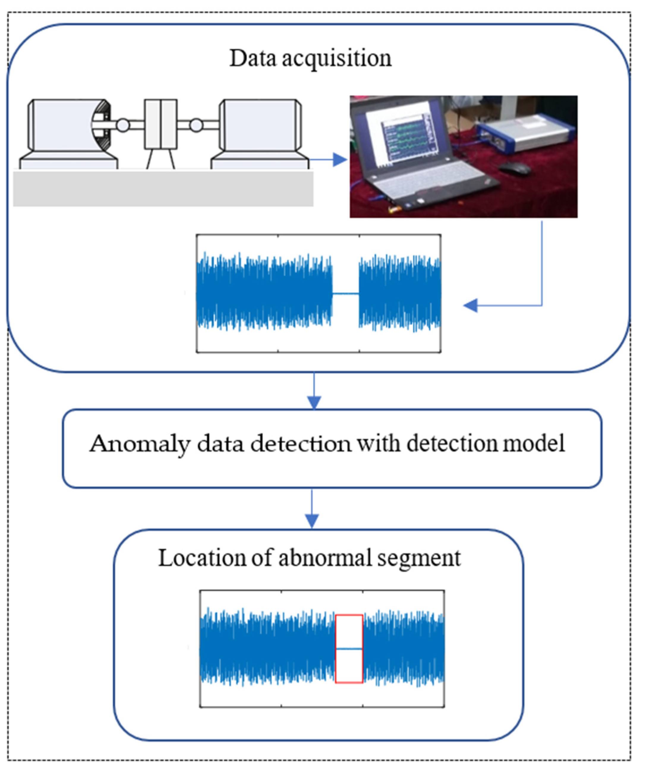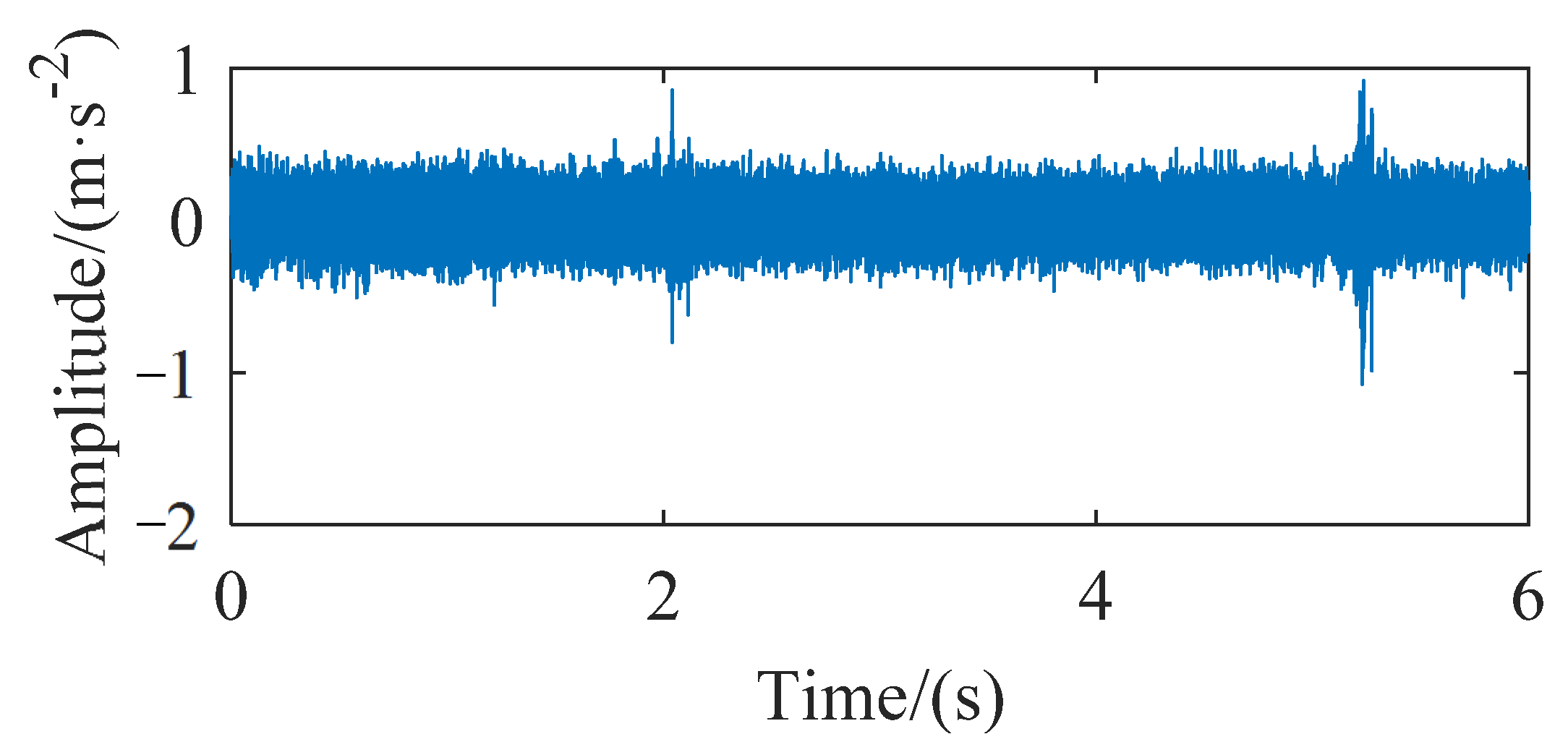In addition, a large number of outliers, missing values and inconsistent data are mixed in the monitoring of big data, resulting in decreased data quality [5]. The direct use of these dirty data will affect the accuracy of fault detection or diagnosis and increase the difficulty of rolling bearings health monitoring. The abnormal data positioning and detection process of rolling bearings is shown in Figure 1. The quality of complete data is reduced due to the existence of missing data. If abnormal polluted data can be detected and subsequent cleaning work can be carried out, the accuracy of state analysis of rolling bearings will be improved.

Outlier detection [6] methods have been widely studied in wind power generation [7], aerospace [8] and other fields. Witayangkurn et al. [9] proposed the use of a Hidden Markov Model (HMM) to detect anomalies in large-scale GPS data. Nonetheless, this approach does not consider the time self-dependence of the observation sequence and requires that the model complexity be predefined, which may bias the unsupervised approach to the analysis [10]. According to the hypothesis of HMM, the HMM model is memoryless and cannot use the information of context. Since it is only related to its previous state, a high-order HMM model has to be established to obtain more information.

There are generally two ideas for PCA [11] in anomaly detection, and both pay special attention to the feature vector corresponding to the smaller eigenvalue. The purpose of the PCA principle is mainly to eliminate the correlation between variables, and assuming that this correlation is linear, it may not obtain good results for nonlinear dependence. The anomaly detection method based on automatic encoder (AE) is a typical reconstruction method that detects anomalies through the error of reconstruction sequence [12,13], while its training data require a large amount of normal data for abnormal recognition scenarios. The statistic-based method assumes a distribution or probability model for data and then the points in the regions of low probability are determined as outliers [14]. In order to recognize the dirty data included in the machinery monitoring data, a new auto regression-generalized, autoregressive conditional heteroskedasticity (AR-GARCH) method is proposed by Lei [15], which can detection local pulse in time series, but it is not validated by other types of abnormal data.

As for distance-based methods, there is the Mahalanobis distance [16], in which each object is calculated and those objects far away from most objects are regarded as outliers. This method may fail to detect outliers in areas with different densities. The local outlier factor (LOF) [17] method is proposed through comparing the density around the data points with the density of their local neighbors. However, in practical application, due to its limitation of only establishing local anomaly models and high complexity, the effect of LOF may not be as good as that of the distance-based method. In the LGBD [18] method, each data point is regarded as an object of the mass and local resultant force (LRF) generated by its neighbors. The main advantage of LGBD is that the detection performance is improved. However, its algorithm complexity is still close to LOF.

Amer et al. [19] proposed an anomaly detection method based on the one-class SVM. Its training set should not be doped with outliers, because the model may match these outliers in the test set. A clustering-based method [20], such as K-means [21], supports vector domain description (SVDD) [22] and density-based spatial clustering of applications with noise (DBSCAN) [23]. They detect outliers which are against clusters, and since the main objective of a clustering method is to find clusters, the cluster-based method may also fail to detect outliers.

The isolation forest (IF) [24], which is based purely on the concept of isolation to detect anomalies without relying on any distance or density measurement, is an unsupervised method without the process of modeling normal data. Since most of the samples do not need to be trained when using this algorithm, the detection model can be constructed by using a data set with a small sample size. IF has strong advantages in detection accuracy and complexity through constructing an isolation tree (iTree) and limiting the depth of the trees [25]. However, the anomaly detection score of the traditional IF is greatly affected by the sample length and capacity. Based on the above analysis, in order to detect and realize the location of abnormal data segments adaptively, a model based on comprehensive features and parameter optimization of the isolation forest, which can identify the abnormal data segment in the vibration signal of rolling element bearings adaptively, is proposed in this paper.

The organizational structure of the rest of this paper is as follows. Section 2 introduces the basic principle of the parameter optimization isolation forest method and comprehensive features. Section 3 shows the steps of the parameter optimization isolation forest and comprehensive characteristics. Section 4 validates and analyzes the proposed method with some data from realistic scenarios. Conclusions are drawn in Section 5.

2. Comprehensive Feature and Parameter Optimized Isolation Forest

2.1. Comprehensive Feature

The time domain statistical feature (TF) of rolling element bearing vibration signals [26] are widely used in signal feature description, such as mean value, kurtosis and root mean square. Statistical characteristic expressions used in this paper are presented in Appendix A. The wavelet packet [27] can not only further process the high frequency part that cannot be subdivided in wavelet transform, but it can also adaptively select the matching frequency band, which can more effectively characterize the signal features. The signal mutation component can be detected more effectively from the perspective of signal frequency domain energy for abnormal data detection. Figure 2 shows the decomposition process of the wavelet packet, here $\gamma$ represents the original signal, A and H, respectively, represent the low and high frequency components, and the subscript is the number of decomposition layers.

Take the n-layer wavelet packet as an example. First, decompose the vibration signal to n layers. The $2^n$ coefficients obtained are $\theta (n,i)(i=1,2,\cdots ,2^n)$. Secondly, the signal reconstructed in the frequency domain is

$$W=W(n,0)+W(n,1)+\cdots +W(n,2^n)$$

(1)

where $W(n,i)$ is the reconstructed signal corresponding to the wavelet packet coefficient.

Next, the total energy $E(n,i)$ of each frequency band signal can be calculated as

$$E(n,i)={{\displaystyle \int \left|W(n,i)\right|}}^{2}dx$$

(2)

When the vibration signal data are abnormal, the energy in each frequency band of the signal will change greatly. Therefore, the energy values of each frequency band can be used to characterize the energy change. Finally, a feature vector representing the change of energy can be expressed as

$$\Omega =[\begin{array}{cccc}E(n,0)& E(n,1)& \cdots & E(n,2^n)\end{array}]$$

(3)

The daubechies wavelet [28] has good regularity—that is, the smoothing error introduced by the wavelet as a sparse basis is not easily detected, which makes the signal reconstruction process smoother. As the number of decomposition layers increases, the difference of signal characteristics becomes more obvious. However, the larger the number of decomposition layers, the greater the distortion of the reconstructed signal. Through the analysis of the studied signal, a 4-layer decomposition can achieve a better feature extraction effect.

Taking signal detection with continuous missing data shown in Figure 3 as an example, a sliding rectangle window with length L is first used to divide the whole data into several segments, and then the data are transformed into several segments using the sliding window.

Then, the TF and WF are easily extracted from each segment. The feature using both TF and WF in the isolation forest model is called the comprehensive feature (CF). Abnormal scores are calculated based on TF, CF and CF in the isolation forest model. The final scores are shown in Figure 4.

It can be seen that whether based on the TF or WF, there are samples whose abnormal scores are very close to their respective adaptive threshold in the final results, which may lead to the final misjudgment of the sample score, and the normal data may be determined as abnormal data. However, when anomaly detection is carried out based on CF, there is no sample score close to their own threshold—that is to say, whether it is above or below the threshold, it is far from the threshold. They are not easily misjudged or confused. Therefore, CF-based scores can extract abnormal data features of rolling element bearings more accurately.

Based on the above analysis, in order to characterize the signal randomness and dynamic behavior, and to comprehensively measure the signal state change from the perspective of statistics and energy, the idea of comprehensive features (CF) is proposed, which combines 15 dimensional time domains and 16 energy features for anomaly detection and recognition.

2.2. Isolation Forest Model

The generation method of the isolation tree (iTree) in the isolation forest (iForest) [24] is relatively simple and fast. It mainly depends on the decision-making principle of random segmentation. The isolation forest (IF) consists of two parts. One part is to establish an isolated forest formed by iTrees, while the other part is to calculate the anomaly score of each research sample. The pseudo-code for establishing the IF model is shown in the Algorithms 1 and 2.

Algorithm 1 iForest (X, t, $\phi$)

Inputs: X-input data, t-number of trees. $\phi$-sub-sampling size

1: Initialize Forest

2: set height limit $I=celing({\log }_2(\phi ))$

3: For i = 1 to t do

4: X’←sample (X, $\phi$)

$5: \mathrm{Forest} \leftarrow \mathrm{Forest} \cup$ iTrees (X’, 0, l)

6: end for

7: return Forest

Output: a set of t iTrees

Algorithm 2 iTree (X, e, l)

Inputs: X-input data, e-current tree height, l –height limit

1:  if e $\ge$ l $\left|X\right|\le 1$ then

2:    return exNode{size ←$\left|X\right|$}

3:  else

4:    let Q be a list of attributes in X

5:    randomly select an attribute split point $q\in Q$

6:    randomly select a split point p from max and min values of attribute q in X

7:    $X_l\leftarrow filter(X,q<p)$

8:    $X_r\leftarrow filter(X,q\ge p)$

9:    return in Node $\{Left\leftarrow \mathrm{iTree}(X_l,e+1,l)\}$,$\{Right\leftarrow \mathrm{iTree}(X_r,e+1,l)\}$

10:  end if

Output: an iTree

Abnormal scores of each research sample can be calculated and evaluated by IF. That is, traverse all iTrees in the forest one by one, extract the node depth of the sample in each iTree, and then obtain the average depth of the sample in the forest. Given a sub-sample set of $\phi$ instances, the average path length of a sample is

$$c(\phi )=\{\begin{array}{cc}2H(\phi -1)-2(\phi -1)/\phi & ,\phi >2\\ 1& ,\phi =2\\ 0& ,\phi <2\end{array}$$

(4)

where $H(k)$ is the harmonic number and it can be estimated by ln(k) + 0.5772156649 (Euler’s constant). $h(\eta )$ is the depth of instance $\eta$ in iTree node, and as $c(\phi )$ is the average of $h(\eta )$ given, we use it to normalize $h(\eta )$. The anomaly score of the instance $\eta$ can be defined as

$$s(\eta )=2^{-\frac{E(h(\eta ))}{c(\phi )}}$$

(5)

where $E[h(\eta )]$ is the average of $h(\eta )$ from a collection of iTrees. The closer the $s(\eta )$ is to 1, the higher the probability that the sample $\eta$ is an abnormal point. The closer it is to 0, the more likely it is a normal sample.

2.3. Parameter Influence Analysis

It is found that when the isolation forest algorithm is used for vibration signal anomaly data detection, the final detection result of the abnormal segment is affected by the length L of input data and sub-sampling size $\phi$. As shown in Figure 5, the abnormal segments detected by the model are marked with a red rectangular box.

Different L and $\phi$ result in different detection results. The missing segment is not completely detected in Figure 5a and the detection of the missing segment in Figure 5b is too long, including some normal values, which are also misjudged as abnormal. The number $\phi$ of the sub-sample set affects the height of the tree and has an important impact on the final abnormal score sequence value, so there may be errors in judging abnormal samples according to the threshold. And different L brings too large or missing anomaly segments and reduced accuracy.

Therefore, it is necessary to optimize L and $\phi$. Then, a parameter optimization isolation forest (POIF) is proposed with PSO [29]. The optimization space of sliding window length L is [500:50:5000] and the optimization space of $\phi$ is [20:20:256]. Of course, the interval of parameter space can be divided into smaller intervals for more accurately locating the abnormal segment, but it will also result in a more complex computation and running time. After setting the parameters, sub-samples with different L are obtained through sliding window segmentation. Then, POIF models with different $\phi$ are established. Finally, the optimal parameters will be obtained as shown in Figure 6.

In order to make the score difference between normal samples and abnormal samples more obvious, the fitness function Q is

$$Q=\mathrm{std}(s)/\mathrm{mean}(s)$$

(6)

where std represents the standard deviation. When Q reaches the maximum, the optimal parameters are obtained. All samples may be distinguished to the greatest extent.

3. Anomaly Vibration Data Detection Flow Based on CF–POIF

3.1. CF-POIF Method

The proposed CF–POIF model has two primary stages: calculate the comprehensive features and obtain the anomaly score. A flow chart of the proposed model is presented in Figure 7.

(1)

The vibration data signal is collected and is segmented by a sliding window from beginning to end to obtain some samples;

(2)

Calculate the comprehensive features of the sub-samples;

(3)

Repeat (1) and (2). According to the principle of maximum standard deviation of abnormal score, the optimal sub-sample length L and sample set size $\phi$ are obtained in the POIF model;

(4)

Calculate the anomaly score of each sample through CF–POIF. Samples whose scores exceed the threshold are judged as abnormal data segments, where the threshold is

$$T=\mathrm{mean}(s)+\alpha \ast \mathrm{std}(s)$$

(7)

According to a rule of thumb for outlier detection [30], $\alpha$ is set to 3 for incorrect data detection.

The computer used for data processing is Windows 10, RAM 16GB. MATLAB is used in this paper for programming code.

3.2. Evaluation Method of CF-POIF

In order to evaluate the advantages and disadvantages of an anomaly detection model, some evaluation indexes are needed as measurement standards. The most commonly used classification index for classification problems is accuracy, which is used to calculate the accuracy of model classification. It returns the proportion of correctly classified samples. The formula is as follows:

$$\mathrm{accuracy}=\frac{n}{M}$$

(8)

where n is the number of correctly predicted samples and M is the total number of samples.

Because the experiment of this paper is anomaly detection, its category data are extremely unbalanced. If we only rely on the index of classification accuracy to judge the quality of the model, it will lead to the prediction of as many test data as possible as normal values, resulting in the loss of significance of the model. The $F_1$ score [31] is an index used to measure the accuracy of two classification models. It takes into account both the precision and recall of the classification model. For binary classification problems, all problems can be divided into negatives (N) and positives (P). The confusion matrix is shown in

Table 1. Confusion matrix.

	Predict Value N	Predict Value P
True value N	TN	FP
True value P	FN	TP

, in which P stands for the abnormal value and N for the normal value. T stands for true and F for false. The $F_1$ score can be calculated as follows:

$$precision=\frac{TP}{TP+FP}$$

(9)

$$recall=\frac{TP}{TP+FN}$$

(10)

$$F_1=\frac{2\cdot precision\cdot recall}{precision+recall}$$

(11)

In order to analyze the effectiveness of the proposed model more objectively and accurately, we use the accuracy and $F_1$ scores to evaluate it together.

4. Simulation and Experimental Validation

4.1. Simulation Validation of Missing Segment Detection

In this case, the vibration signal has been collected from a test rig of wheelset bearing in our laboratory, which is carried out to test the validity of the proposed method. The test rig structure is presented in Figure 8. The sampling frequency Fs is 25.6 kHz and the set speed is 465 r/min.

Data collected in the outer ring fault experiment are shown in Figure 9a. The signal is complete and there are no abnormal data. In fact, owing to the network data transmission loss, cable failures or sensor failure, the actual data of missing segments are usually replaced with 0, NaN values, or environment noise [32], which damages the completeness of the data. In order to simulate the possible data loss during the experiment, the complete data are artificially processed to make the data miss some points. Then, a missing segment is produced by replacing the actual data with Gaussian white noise as shown in Figure 9b.

The proposed method is used to detect the abnormal data segment. The CF has 31 dimensions in total, the optimal sample length L is 2 400, and the optimal sub-sample set size $\phi$ is 60. Figure 9c shows the abnormal score of each sub-sample in the CF–POIF model, where A represents the abnormal sample, N represents the normal sample, and T is the threshold. Obviously, the abnormal score of two samples exceeds T. The final abnormal location in the time domain is shown in Figure 9d, where the abnormal segments are marked automatically by using a red rectangular box.

In order to demonstrate the advantages of the proposed model, compare it with other methods. The CF combined with LOF is called CF–LOF and the CF combined with IF with parameters not optimized is called CF–IF. The k nearest neighborhood value is 5 in LOF. Their detection results are shown in Figure 9.

It can be clearly seen that only part of the missing segment is marked and there is still missing data that have not been detected in Figure 10, so the reliability of the predict results is insufficient. Various models are compared with quantitatively, normal and abnormal data points and are counted in the test results of each model. It is found that the accuracy and $F_1$ score are highest among three methods in

Table 2. Accuracy and $F_1$ score of signal.

Methods	CF-IF	CF-LOF	CF-POIF
accuracy	0.9928	0.9870	0.9948
$F_1$ score	0.8406	0.7059	0.9091

, indicating that the proposed model has the best detection performance for abnormal missing data.

4.2. Experimental Validation of Abnormal Data Segment Detection

In this section, the abnormal data segment naturally formed in the bearing fault experiment of Case Western Reserve University [33] is used to test the effectiveness of the proposed model. As shown in Figure 11, the test bench consists of a 2 HP motor (left), a torque sensor/encoder (middle), a dynamometer (right) and control electronics (not shown). During the experiment, the rotating speed is 1730 rpm, and the sampling frequency is 48 kHz. There is a fault in the bearing inner ring and the fault size is 0.014 inch. Vibration signals are collected at both the drive end and the fan end.

The drive end vibration signal is shown in Figure 12, while the signal from 0.336–0.666 s is contaminated by an impurity signal under the influence of uncertain factors, which may be caused by electromagnetic interference. In order to observe whether it is disturbed by abnormal signals from 0.336–0.666 s, Figure 12b shows the local enlarged signal of Figure 12a. Distorted data can be clearly found between 0.336–0.666 s in Figure 12b.

If intelligent anomaly data detection is not carried out, the direct use of the data may cause inaccurate results from various models. After this signal is solved by the proposed CF–POIF method, L = 4650, $\phi$ = 240 are obtained. Then, calculate the anomaly score of each sample and map it back onto the time domain waveform. The final positioning result only exists in 0–1 s; no abnormal samples are identified in other time periods in Figure 13. Therefore, only the identification and positioning results within 0–1 s are displayed for clear observation detection results.

As shown in Figure 14a, the proposed model automatically marks the detection result with a red rectangular box, which accurately locates the abnormal segment. A detection result between 0–1 s of CF-IF with a random parameter combination is shown in Figure 14b, and the parts marked with two red ellipses are not recognized. There are still many data not marked by the red rectangular box between 0.4–0.6 s, indicating that the method does not detect all outliers. The part marked with one red ellipse in Figure 14c is not recognized. So, the accuracy of CF–LOF is not as good as CF–POIF, indicating that the LOF method may fail in the anomaly detection of complex and large data sets since it calculates the sub-sample anomaly score based on the method of spatial local density, which is affected by the spatial location of neighbor samples. If the data set is composed of multiple density sets, the sample in the area with dense anomaly samples can be easily recognized as normal because its neighbors are similar and close to it, which is the deficiency of the LOF anomaly detection algorithm, while the POIF method does not have the above problems. It randomly selects the feature dimension for division and calculates the anomaly score according to the division path depth with strong independence—that is, the POIF is not easily affected by other samples.

The accuracy and $F_1$ score from three methods are calculated in

Table 3. Accuracy and $F_1$ score of drive end vibration signal.

Methods	CF-IF	CF-LOF	CF-POIF
Accuracy	0.9816	0.7300	0.9942
$F_1$ score	0.6129	0.4905	0.9199

. We can conclude that the proposed model has the best effect for this type of abnormal data detection.

The fan end signal is shown in Figure 15. It is difficult to find abnormal data segments through manual observation, while the signal from 0.336–0.666 s is also contaminated by impurity signals. The proposed model is applied for dirty data detection and cleaning. After optimization in the POIF model, L = 2650 and $\phi$ = 120 are obtained. The final abnormal positioning result based on CF–POIF is only within 0–1 s.

As can be seen in Figure 16a, the detection result of the proposed model is automatically marked with a red rectangular box, although some points from 0.662–0.666 s are regarded as normal points. However, such a small error is allowed for the final abnormal section detection result. A detection result between 0–1 s of the CF–IF is shown in Figure 16b, where parts marked with six red ellipses are not recognized. The proportion of abnormal sub-signals may increase due to the small length of the sub-samples. It is also possible that the shorter the length of sub-samples, the more similar their features, which makes it difficult to distinguish anomalies.

The CF–LOF method cannot identify all the abnormal segments, and the parts marked with red ellipses are not correctly identified in Figure 16c. This result is also caused by the disadvantages of the LOF, which have been explained in detail above.

For comparing various models quantitatively, the accuracy and $F_1$ scores of three abnormal detection methods are displayed in

Table 4. Accuracy and $F_1$ score of fan end signal.

Methods	CF-IF	CF-LOF	CF-POIF
accuracy	0.8005	0.8676	0.9992
$F_1$ score	0.5668	0.7928	0.9840

. The accuracy and $F_1$ score of CF–POIF improve much more than the other two methods. The proposed model can be considered to effectively identify abnormal data from the fan end vibration signal.

4.3. Experimental Validation of Drift Data Segment Detection

The test is carried out based on the rolling and vibration test rig of single wheelset. Its field assembly and structural diagrams are shown in Figure 17. The test rig is composed of the loading reaction frame, actuator, bogie frame, wheelset system, rail wheels and other components. The sampling frequency is 25.6 kHz. As shown in Figure 18, the data drifted greatly nearby 0.8 s may be due to the looseness of the sensor or abnormal shaking of the train wheel set. The data quality decreases and the result of the fault diagnosis is probably incorrect from analysis of these poor-quality data. Thus, these data should be detected by the proposed method to improve the data quality.

The detection results of the CF–POIF, CF–IF, and CF–LOF methods are shown in Figure 18, respectively. The detection results of the proposed methods are marked out using a red rectangle in Figure 18a. It can be seen that the position at the beginning of the drift is successfully detected, while in Figure 18b, although some abnormal segments can be identified at the beginning of slip by using CF–IF, abnormal values are also detected at other time points, which is obviously inaccurate. The CF–LOF method detects three time periods, but none of them is the time period of the slip. Given all of that, the proposed method yields good performance in abnormal drift segment detection.

4.4. Experimental Validation of Random Large Impact Interference Data Segment Detection

In this case, the validity of the proposed method will be further evaluated using real monitoring data from our research group in 2017. In the tracking test stage of the standard EMU, when the train is running on a railway, the key rotating parts of the bogie are monitored and the collected vibration data are shown in Figure 19. The vibration data at 2 s and 5.2 s are disturbed by random large impact, resulting in a larger amplitude than other time periods. This may be caused by abnormal vibration of the wheel set. In addition, pits or bulges on the rail line will also produce a large random impact when the train runs here.

Thus, the proposed method is used to detect the abnormal segment for data cleaning. As shown in Figure 20a, the abnormal data at 2 s and 5.2 s are detected as incorrect data and marked out using a red rectangle, which almost agrees with the facts. For comparison, four methods—CF–IF, CF–LOF, Mahalanobis distance and K-means—are used to detect incorrect data.

Although the CF–IF and CF–LOF methods have detected some impact values at two time points, there is a case of misjudging the normal value as an abnormal value near 2 s with both of them. The recognition result near 5.2 s is that only parts of the abnormal values are identified successfully, and the remaining abnormal values are not detected successfully.

As can be seen in Figure 20d, the Mahalanobis distance method successfully detects the impact near 2 s, but it fails to detect all abnormal values at 5.2 s. Only boundaries with a large amplitude of impact are marked with two red rectangles. It cannot identify all abnormal values, as shown in one red ellipse in Figure 20e. Obviously, the Mahalanobis distance method also fails to detect the incorrect data because of its limitation with respect to the description of the contour of the Gaussian cluster.

The result of the K-means is shown in Figure 20f. Consequently, almost all the data marked in red are detected as abnormal data. Obviously, the K-means method cannot detect anomaly data accurately either because this method, whose focus is on clustering, has a good effect on those samples with obvious feature differences, while the features of the data in cluster space may not be obvious, which leads to the failure of this method.

5. Conclusions

In this paper, a CF–POIF model is proposed to detect the abnormal vibration data of rolling element bearings. Through simulation and experimental analysis, the effectiveness of the proposed model in detecting the abnormal loss and distortion in the vibration signals of rolling element bearings is verified. The following conclusions can be drawn:

(1)

By comparing CF–IF and CF–POIF, we can conclude that the maximum standard deviation of abnormal score as the fitness function can effectively optimize L and $\phi$ in the POIF, and these parameters greatly affect the final detection results. The CF–POIF method is effective for vibration signal anomaly data detection.

(2)

Comparison between CF–POIF and CF–LOF shows that the anomaly score of samples in CF–LOF will be affected by the neighborhood samples, while it will not be effected by neighborhood samples in CF–POIF.

This paper presents a new approach to the abnormal detection of vibration data and lays a preliminary foundation for the accurate use of subsequent data. Meanwhile, it provides some reference for anomaly detection of data streams in other fields.

References

1. Liu, C.; Tan, J.; Huang, Z. Fault Diagnosis of Rolling Element Bearings Based on Adaptive Mode Extraction. Machines 2022, 10, 260. [Google Scholar] [CrossRef]
2. Feng, K.; Wang, K.; Ni, Q. A phase angle based diagnostic scheme to planetary gear faults diagnostics under non-stationary operational conditions. J. Sound Vib. 2017, 408, 190–209. [Google Scholar] [CrossRef]
3. Zhang, X.; Hu, N.; Zhe, C.; Hua, Z. Vibration data recovery based on compressed sensing. Acta Phys. Sin. 2014, 63, 200506. [Google Scholar] [CrossRef]
4. Lei, Y.; Xu, X.; Cai, X.; Li, N.; Kong, D.; Zhang, Y. Research on data quality assurance for health condition monitoring of machinery. J. Mech. Engineer. 2021, 57, 1–9. [Google Scholar]
5. Dong, Z.; Jia, H. Outlier detection method for thermal process data based on EWT-LOF. Chin. J. Sci. Inst. 2020, 41, 126–134. [Google Scholar]
6. Manobel, B.; Sehnke, F.; Lazzús, J.A. Wind turbine power curve modeling based on Gaussian processes and artificial neural networks. Renew. Energ. 2018, 125, 1015–1020. [Google Scholar] [CrossRef]
7. Qi, M.; Fu, Z.; Chen, F. Outliers detection method of multiple measuring points of parameters in power plant units. Appl. Thermal Eng. 2015, 85, 297–303. [Google Scholar] [CrossRef]
8. Peng, X.; Pang, J.; Peng, Y.; Liu, D. Review on anomaly detection of spacecraft telemetry data. Chin. J. Sci. Inst. 2016, 37, 1929–1945. [Google Scholar]
9. Witayangkurn, A.; Horanont, T.; Sekimoto, Y.; Shibasaki, R. Anomalous event detection on large-scale GPS data from mobile phones using hidden markov model and cloud platform. In Proceedings of the 2013 ACM Conference on Pervasive and Ubiquitous Computing Adjunct Publication, Online, 8 September 2013; pp. 1219–1228. [Google Scholar]
10. Qarout, Y.; Raykov, Y.P.; Little, M.A. Probabilistic Modelling for Unsupervised Analysis of Human Behaviour in Smart Cities. Sensors 2020, 20, 784. [Google Scholar] [CrossRef] [Green Version]
11. Shyu, M.L.; Chen, S.C.; Sarinnapakorn, K.; Chang, L. A novel anomaly detection scheme based on principal component classifier. In Proceedings of the 3rd IEEE International Conference on Data Mining (ICDM), Melbourne, FL, USA, 19–22 November 2003. [Google Scholar]
12. Zhang, C.; Song, D.; Chen, Y.; Feng, X.; Lumezanu, C.; Cheng, W.; Ni, J.; Zong, B.; Chen, H.; Chawla, N.V. A deep neural network for unsupervised anomaly detection and diagnosis in multivariate time series data. In Proceedings of the Conference on Artificial Intelligence 2019, Honolulu, HI, USA, 27 January–1 February 2019; pp. 1409–1416. [Google Scholar]
13. Zong, B.; Song, Q.; Min, M.R. Deep autoencoding gaussian mixture model for unsupervised anomaly detection. In Proceedings of the International Conference on Learning Representations (ICLR), Vancouver, BC, Canada, 30 April–3 May 2018; pp. 1–19. [Google Scholar]
14. Shuster, J.J. Student t-tests for potentially abnormal data. Statist. Med. 2009, 28, 2170–2184. [Google Scholar] [CrossRef] [Green Version]
15. Lei, Y.; Zhou, X.; Xu, X.; Jia, F. A dirty data recognition method for machinery condition monitoring in big data era. In Proceedings of the 43rd Annual Conference of the IEEE Industrial Electronics Society (IECON), Beijing, China, 29 October–1 November 2017; pp. 7061–7066. [Google Scholar]
16. Wang, F.; Gao, X.; Jia, X. An Anomaly Detection Ensemble Algorithm for Power Dispatching Data Based on Log-interval Isolation. Power Syst. Tech. 2021, 45, 4818–4827. [Google Scholar]
17. Breunig, M.M.; Kriegel, H.P.; Ng, R.T.; Sander, J. LOF: Identifying density-based local outliers. In Proceedings of the International Conference on Management of Data, Dallas, TX, USA, 16 May 2000; Volume 1, pp. 93–104. [Google Scholar]
18. Xie, J.; Xiong, Z.; Dai, Q.; Wang, X.; Zhang, Y. A local gravitation-based method for the detection of outliers and boundary points. Knowl. -Based Syst. 2020, 192, 105331. [Google Scholar] [CrossRef]
19. Amer, M.; Goldstein, M.; Abdennadher, S. Enhancing one-class support vector machines for unsupervised anomaly detection. In Proceedings of the 19th ACM SIGKDD International Conference on Knowledge Discovery and Data Mining, Chicago, IL, USA, 11–14 August 2013; pp. 8–15. [Google Scholar]
20. Pamula, R.; Deka, J.K.; Nandi, S. An outlier detection method based on clustering. In Proceedings of the International Conference Emerging Applications of Information Technology, Kolkata, India, 19–20 February 2011; Volume 2, pp. 253–256. [Google Scholar]
21. Yoon, K.A.; Kwon, O.S.; Bae, D.H. An approach to outlier detection of software measurement data using the k-means clustering method. In Proceedings of the First International Symposium on Empirical Software Engineering and Measurement (ESEM 2007), Madrid, Spain, 20–21 September 2007; pp. 443–445. [Google Scholar]
22. Chen, G.; Zhang, X.; Wang, Z.J.; Li, F. Robust support vector data description for outlier detection with noise or uncertain data. Knowl. Based Syst. 2015, 90, 129–137. [Google Scholar] [CrossRef]
23. Li, L.; Gariel, M.; Hansman, R.J.; Palacios, R. Anomaly detection in onboard-recorded flight data using cluster analysis. In Proceedings of the IEEE/AIAA 30th Digital Avionics Systems Conference, Seattle, WA, USA, 16–20 October 2011; pp. 1–11. [Google Scholar]
24. Liu, F.; Ting, K.; Zhou, Z. Isolation Forest. IEEE Data Min. 2009, 8, 413–422. [Google Scholar]
25. Yang, J.; Wang, L.; Song, D. Diagnostic method of zero-point shifting of wind Turbine yaw angle based on isolated forest and sparse Gaussian process regression. Proc. CSEE 2021, 41, 6198–6211. [Google Scholar]
26. Xu, X.; Lei, Y.; Li, Z. An Incorrect data detection method for big data cleaning of machinery condition monitoring. IEEE Trans. Ind. Electron. 2019, 67, 2326–2336. [Google Scholar] [CrossRef]
27. Beale, C.; Niezrecki, C.; Inalpolat, M. An adaptive wavelet packet denoising algorithm for enhanced active acoustic damage detection from wind turbine blades. Mech. Syst. Signal Process. 2020, 142, 106754. [Google Scholar] [CrossRef]
28. Alejandro, S.; Carlos, G.G.; Miguel, R.G. Improving the sensitivity of early rub detection in rotating machines with an adaptive orthogonal filter. Mech. Syst. Signal Process 2022, 171, 108900. [Google Scholar]
29. Cai, Z.; Dang, Z.; Wen, M.; Lv, Y.; Duan, H. Application of Compressed Sensing Based on Adaptive Dynamic Mode Decomposition in Signal Transmission and Fault Extraction of Bearing Signal. Machines 2022, 10, 353. [Google Scholar] [CrossRef]
30. Kriegel, H.P.; Kroger, P.; Schubert, E.; Zimek, A. Outlier detection in arbitrarily oriented subspaces. In Proceedings of the 12th International Conference on Data Mining (ICDM), Brussels, Belgium, 10–13 December 2012; Volume 12, pp. 379–388. [Google Scholar]
31. Powers, D.M.W. Evaluation: From precision, recall and F-measure to ROC, informedness, markedness and correlation. J. Mach. Learn. Tech. 2020, 2, 37–63. [Google Scholar]
32. Wang, Z.; Ho, D.W.C.; Liu, X. Variance-constrained filtering for uncertain stochastic systems with missing measurements. IEEE Trans. Autom. Control 2003, 48, 1254–1258. [Google Scholar] [CrossRef] [Green Version]
33. Su, H.; Xiang, L.; Hu, A.; Xu, Y.; Yang, X. A novel method based on meta-learning for bearing fault diagnosis with small sample learning under different working conditions. Mech. Syst. Signal Process 2022, 169, 108765. [Google Scholar] [CrossRef]
Figure 1. Flow of bearing vibration signal acquisition and anomaly data detection.
Machines 10 00459 g001
Figure 2. Wavelet packet decomposition tree.
Machines 10 00459 g002
Figure 3. The data segmentation using a sliding rectangle window.
Machines 10 00459 g003
Figure 4. Anomaly score based on TF, WF and CF.
Machines 10 00459 g004
Figure 5. Parameter influence analysis. (a) L = 1900, φ = 20; (b) L = 1900, φ = 200; (c) L = 3000, φ = 100; (d) L = 2500, φ = 100.
Machines 10 00459 g005aMachines 10 00459 g005b
Figure 6. Process of POIF.
Machines 10 00459 g006
Figure 7. Flow chart of the proposed CF-POIF.
Machines 10 00459 g007
Figure 8. The test rig of wheelset bearing.
Machines 10 00459 g008
Figure 9. Detection result with CF-POIF. (a) complete signal; (b) signal with missing segment; (c) abnormal score; (d) detection result.
Machines 10 00459 g009
Figure 10. Detection results with other methods. (a) CF-IF; (b) CF-LOF.
Machines 10 00459 g010
Figure 11. The experimental setup.
Machines 10 00459 g011
Figure 12. (a) Drive end vibration signal. (b)Signal from 0.336–0.666 s.
Machines 10 00459 g012
Figure 13. Abnormal data detection results of drive end signal with proposed method.
Machines 10 00459 g013
Figure 14. Abnormal data detection results of drive end signal. (a) CF-POIF; (b) CF-IF; (c) CF-LOF.
Machines 10 00459 g014aMachines 10 00459 g014b
Figure 15. Fan end vibration signal.
Machines 10 00459 g015
Figure 16. Abnormal data detection results of fan end signal. (a) CF-POIF; (b) CF-IF; (c) CF-LOF.
Machines 10 00459 g016
Figure 17. Rolling and vibrating test rig.
Machines 10 00459 g017
Figure 18. Detection results of drift data. (a) CF-POIF; (b) CF-IF; (c) CF-LOF.
Machines 10 00459 g018
Figure 19. The signal from the EMU.
Machines 10 00459 g019
Figure 20. Detection results of random large impact data. (a) CF-POIF; (b) CF-IF; (c) CF-LOF; (d) Mahalanobis distance; (e) local enlarged result with Mahalanobis distance; (f) K-means.
Machines 10 00459 g020aMachines 10 00459 g020b