Article

Improved DBSCAN Spindle Bearing Condition Monitoring Method Based on Kurtosis and Sample Entropy

1
School of Mechanical and Precision Instrument Engineering, Xi’an University of Technology, Xi’an 710048, China
2
Luoyang Bearing Science & Technology Co., Ltd., Luoyang 471039, China
3
Aviation Industry Corporation of China Co., Ltd., Xi’an 710089, China
*
Author to whom correspondence should be addressed.
Machines 2022, 10(5), 363; https://doi.org/10.3390/machines10050363
Submission received: 8 April 2022 / Revised: 1 May 2022 / Accepted: 5 May 2022 / Published: 10 May 2022

Abstract

:
An improved density-based spatial clustering of applications with noise (IDBSCAN) analysis approach based on kurtosis and sample entropy (SE) is presented for the identification of operational state in order to provide accurate monitoring of spindle operation condition. This is because of the low strength of the shock signal created by bearing of precision spindle of misalignment or imbalanced load, and the difficulties in extracting shock features. Wavelet noise reduction begins by dividing the recorded vibration data into equal lengths. Features like kurtosis and entropy in the frequency domain are used to generate feature vectors that indicate the bearing operation state. IDBSCAN cluster analysis is then utilized to establish the ideal neighborhood radius (Eps) and the minimum number of objects contained within the neighborhood radius (MinPts) of the vector set, which are combined to identify the bearing operating condition features. Finally, utilizing data from the University of Cincinnati, the approach was validated and assessed, attaining a condition detection accuracy of 99.2%. As a follow-up, the spindle’s vibration characteristics were studied utilizing an unbalanced bearing’s load bench. Bearing state recognition accuracy was 98.4%, 98.4%, and 96.7%, respectively, under mild, medium, and overload circumstances, according to the results of the experimental investigation. Moreover, it shows that conditions of bearings under various unbalanced loads can be precisely monitored using the proposed method without picking up on specific sorts of failures.

1. Introduction

Rolling bearings are a critical component of a precision spindle, and their operational condition directly impacts the spindle’s performance. Alternating loads, manufacturing flaws, incorrect installation, and other reasons can cause rolling bearings to fail [1,2]. Spindle system downtime and poor machine quality can ensue. The non-linear motion of the spindle system is affected by the bearing’s loading pattern [3,4,5]. Consequently, a significant issue in spindle system condition monitoring is how to determine the operating status of rolling bearings under various loading patterns.
Vibrations from a spindle bearing caused by a rolling bearing are not linear and smooth; this makes it difficult to monitor the bearing’s working condition. Other causes for this include the bearing material and friction coefficient, as well as the noise from the spindle. Eccentricity and misalignment of bearings and system components, such as spindles, can be caused by a misplaced installation or an imbalanced load. In general, these phenomena shorten the service life of bearings, alter the stability of the working system, and reduce the lubrication performance and precision of machined components [6,7,8]. However, the focus of current research has shifted away from signal processing in favor of studying the dynamic performance of bearings under misaligned or unbalanced load conditions [9,10,11,12]. It is also difficult to monitor bearings running state under imbalanced loads since the early bearings have a less significant shock effect on the vibration signal. Condition monitoring can only be solved by figuring out how to properly extract spindle system vibratory characteristics while it is operating under load with a misalignment or an imbalanced load.
The extraction of early faint fault characteristics from rolling bearings has progressed significantly over the last few years [13,14,15,16]. Scholars have made improvements on traditional feature extraction algorithms. Castellani et al. first extracted the RMS, skewness, kurtosis, crest factor, and peak value of the preprocessed acceleration signal, analyzed the damage detection ability of a single feature using ANOVA, and realized the data visualization using PCA. Finally, the target is distinguished from the reference wind turbine using a novelty metric based on Mahalanobis distance [17]. Kurtosis, a statistical measure of the distribution of random variables, is increasingly being employed in the detection of bearing cracks. Time domain kurtosis of the wheel bearing vibration signal and the fault frequency were used as feature vectors for spectral kurtosis analysis by Chen Bin et al. [18]. Rohani Bastami and Bashari proposed a wavelet-based impulse response method for damped single-degree-of-freedom systems, and then found the optimal damping ratio by maximizing the ratio of the peak of spectral kurtosis (SK) to the mean value of SK. Finally, the method is applied to the simulated vibration signal of the defective REB and the experimental vibration signal of the defective REB. The results show that the method outperforms the SK calculation based on STFT and Morlet wavelet in detecting the resonance band of the vibration signal [19]. Bearing fracture classification under varied flaws was then completed using a support vector machine (SVM). Bearing degradation can be detected by analyzing SK and correlation coefficients, which can detect early faults in the presence of concealed noise and pinpoint their location by Tian Jing et al. [20]. Zhong et al. improved the calculation method of kurtosis and negative entropy, and proposed an index based on weighted residual regression, thereby reducing the sensitivity of kurtosis and entropy to impulse noise. Finally, it is verified in gear and bearing degradation evaluation, and the results show that the improved state index has better early fault detection ability and monotonic trend ability [21]. It is worth noting that entropy algorithms quantify the complexity of data, making them useful for a wide range of structural health monitoring and defect identification tasks [22,23]. Sandoval et al. used multiple entropy indexes to represent bearing vibration signals under different health conditions and compared them with conventional indexes. The results show that entropy indexes (EIs) can more accurately distinguish damaged bearings of low-speed bearings. Furthermore, the results show that the combination of conventional metrics and entropy-based metrics also contributes to more reliable diagnosis [24]. Without knowing where the data for the target series came from, sample entropy (SE) is applied in order to assess its randomness [25]. In the realm of bearing condition monitoring and problem diagnostics, certain applications have thus been found [26,27]. Support vector machines were used to classify the LMD, sample entropy, and energy ratio values that Han provided as a diagnostic technique [26]. Wang used generalized refined combined multiscale sample entropy to extract fault features and supervised isometric mapping to reduce dimensionality before employing support vector machines (GOS-SVM) and grasshopper optimization algorithms to finish the diagnosis of rolling bearing faults [27]. Researchers, on the other hand, found that the most obvious types of bearing cracks, such as inner ring, outer ring, and rolling element faults, could be extracted using feature extraction. This method may not be able to accurately detect a bearing’s operating state when the bearings do not have problems but are an unbalanced load because of improper assembly and other issues. When dividing raw data at different scales, scale factors must be considered, and the division effect tends to be unpredictable as the data length grows. As a result, the kurtosis and entropy values of the vibration signal are studied in this work as state characteristics of the bearing under imbalanced loading conditions. As a result, determining the condition of the bearings at various levels of misalignment is a problem.
In the field of early fault diagnosis of rolling bearings, machine learning-based fault diagnosis methods have garnered considerable attention [28,29,30,31,32]. Cluster analysis, as one of the unsupervised learning modules in machine learning, is gaining traction in practical applications such as bearing crack diagnosis. Du [33] proposed a density-peak clustering (PCA) method based on k-nearest neighbor and major component analysis, which was performed on high-level data for dimension reduction and combined with k-nearest neighbor and density-peak clustering algorithms, and finally the proposed method’s validity was verified using synthetic data. The limitation of this method, however, is that it was not validated against actual engineering data, and the method’s weakness is that it has not been validated against real-world engineering data. DBSCAN is widely used as a density-based spatial clustering algorithm in the field of condition monitoring and fault diagnosis. S. Kerroumi [34] came up with a density-based dynamic clustering of noise application space (D-DBSCAN) dynamic classification method that automatically recognizes families under new patterns and creates new families based on anomalies for monitoring nodes caused by bearing cracks. However, the method does not automatically pick the Eps and MinPts parameters. Hai Li [35] came up with a way to classify faults that used adaptive symmetry point patterns and density-based spatial clustering for noise applications (ASDP-DBSCAN). Using an improved genetic algorithm, the symmetry dots pattern (SDP) parameters were found out. Then, the vibration signal was reconstructed by using the SDP pattern. Finally, the difficult problem of automatically selecting parameters for DBSCAN was solved by using the single-degree-of-freedom parameter selection method. This method is good for fault detection, but it also makes the computer work harder because of the complexity of the SDP pattern conversion. The KANN-DBSCAN algorithm proposed by Li [36] generates candidate Eps and MinPts parameters based on the dataset’s distribution characteristics. It can find a stable interval for the cluster number variation of the clustering results automatically and use the minimum density threshold in the interval as a criterion for discriminating the optimal Eps and MinPts parameters. Although the accuracy of this method is relatively high, as the volume of data grows, so does the computational complexity and cost. If the density is not uniform, there will be no solution. Therefore, the clustering algorithm can be improved in order to increase the efficiency of its practical application.
An improved DBSCAN method based on kurtosis and sample entropy is suggested in this paper to monitor and categorize spindle bearings’ unbalanced load operating conditions. The following is the general layout of this manuscript: Following the extraction of kurtosis and frequency domain sample entropy values, the improved DBSCAN algorithm’s parameters Eps and MinPts are analyzed in Section 2 to determine the improved DBSCAN algorithm’s parameters. An IMS (Intelligent Maintenance System) bearing test stand created by University of Cincinnati is used to validate the proposed technique in Section 3, which extracts feature information for each failure mode and passes it along as an input vector to the clustering algorithm. Finally, the method’s accuracy in identifying states is reported to be 99.2%. Construction of an unbalanced bearing’s load test bench was the focus of Section 4. Vibration data was collected at three points on the outer ring of the bearing. The condition monitoring mechanism described in this work was then used to process the signals. Experiments showed that under light, medium, and heavy load circumstances, the accuracy of condition recognition was 96.7% to 99.4% accordingly. These results, in conjunction with those found in Section 3 and Section 4, show that the condition monitoring method is useful not only for identifying certain types of operating problems, but also for detecting minor changes in the operation of unbalanced loads in bearings.

2. Algorithm Design

2.1. Feature Extraction Method Based on Kurtosis and Sample Entropy

2.1.1. Kurtosis

An important concept in probability theory and statistics known as kurtosis is used to compute the kurtosis of a probability distribution and to reflect the convexity of a signal probability density function’s top. Since the probability of big values increases with increasing kurtosis, it is a useful tool for detecting impulse information in non-stationary signals.
According to Equation (1), the so-called kurtosis indicator is generally defined as the fourth-order center moment divided by squared variance.
K u = 1 n i = 1 n ( x i μ ) 4 ( 1 n i = 1 n ( x i μ ) 2 ) 2
where, K u is the kurtosis, which indicates a dimensionless indicator; x i represents the ith value of the samples, n represents the length; μ is the mean of the samples. With a kurtosis of 3, this is a normal distribution. The kurtosis reflects the sharpness of the peaks, the kurtosis K u = 3 is called the normal distribution, The kurtosis K u > 3 is called the thick tail, the kurtosis K u < 3 is called the fine tail. The impulse response generated by the vibration signal is small, because the bearing itself has small defects in the rolling bearing misplaced installation or unbalanced load operation. The kurtosis value is generally less than 3 or slightly greater than 3, and the vibration signal will produce a weak shock due to the different degrees of unbalanced load, so kurtosis in the time domain waveform can be used as a typical quantity of state monitoring.

2.1.2. Sample Entropy

The Sample Entropy (SE) of a time series is a statistical measure of its complexity that is used to describe the probability of a sequence generating new patterns when the dimension is altered. SE is an upgraded version of the Approximate Entropy (AE) algorithm. Unlike AE, SE is not dependent on the length of the data and has a higher level of consistency. According to the definition of sample entropy, the larger the likelihood of generating a new pattern, the greater the sample entropy value. For example, given a time series of vibration signals u = u(1), u(2)…u(N), reconstruct the sequence to obtain an m-dimensional sequence B = X(1), X(2)…X(N − m + 1), when the dimension of the reconstructed sequence is m + 1, then the sequence at this time is A = X(2), X(3)…X(N − m + 2), and the self-similar probability P = A/B is obtained, so the approximate entropy of the average value of log P. Moreover, the calculation result of the approximate entropy includes the comparison between the reconstruction vectors, so there is a certain deviation. The SE is derived by first summing the self-similar probabilities P and then computing the logarithm of P, avoiding the comparison of reconstruction vectors. The advantage of SE is that it is independent of the sample length and has a higher degree of consistency, making it more sensitive to detecting minor signal variations. As a result, this article processes the recorded bearing eccentric load vibration data for noise reduction and then extracts the sample entropy from the corrected data. The sample entropy is calculated in the following manner:
Suppose a time series containing N data points: { x ( i ) } , 1 i N
(1)
Given a sequence of m-dimensional vectors
x ( i ) = x _ 1 ( i ) , x _ 1 ( i + 1 ) , , x _ 1 ( i + m 1 )
where i = 1 , 2 , , N m + 1 .
(2)
As indicated in Equation (3), we can define the maximum difference between the elements corresponding to the vector X ( i ) and vector X ( j ) as the distance z between them, that is:
d [ X ( i ) , X ( j ) ] = max k = 0 ~ m 1 [ x ( i + k ) x ( j + k ) ]
where, d [ X ( i ) , X ( j ) ] is the distance between vector X ( j ) and vector X ( i ) .
Given a similar tolerance threshold r, where r is assumed to be between 0.2 and 0.25 times the series’ standard deviation. Calculate the number of distances between each corresponding element of X ( i ) and X ( j ) that exceeds r, recorded as: N u m d [ X ( i ) X ( j ) ] < r , and calculate its ratio to the total number of vectors N m , recorded as S v i m ( r ) , as shown in Equation (4):
S v i m ( r ) = N u m d [ X ( i ) X ( j ) ] < r N m
Record the average of the N m + 1 equations in Equation (4) as S v m ( r ) , as shown in Equation (5):
S v m ( r ) = 1 N m i = 1 N m S v i m ( r )
where S v m ( r ) is the probability of obtaining m points for two sequences at distance r.
(3)
Expand the value of m, and repeat steps: (1)~(3), the result is shown in Equation (6):
S v m + 1 ( r ) = 1 N m i = 1 N m S v i m + 1 ( r )
(4)
Therefore, the sample entropy of the sequence { x ( i ) } is calculated as shown in Equation (7):
S a m p E n ( m , n ) = lim N { ln S v m + 1 ( r ) S v m ( r ) }
However, the data length N given in the paper is a finite value, so Equation (7) is rewritten as:
S a m p E n ( m , n ) = ln S v m + 1 ( r ) S v m ( r )
The frequency domain sample entropy is proposed in this paper based on the computation of sample entropy. In order to determine the sample entropy value, the frequency domain amplitude of each group is combined with Equations (2)–(8) and the sample entropy value is derived using Equations (2)–(8) and the original vibration signal, as illustrated in Figure 1.

2.2. IDBSCAN Clustering Algorithm

The conventional density-based spatial clustering algorithm needs the identification of two parameters, MinPts and Eps, which characterize how tightly the data points are distributed and separate dense regions into clusters to generate the greatest collection of points that fulfill the linked density. As a result, the MinPts and Eps parameters are extremely sensitive to the DBSCAN algorithm, which might result in poor or erroneous clustering. Therefore, the DBSCAN algorithm is improved for the distribution of intelligent spindle vibration characteristics as shown in Figure 2.

2.2.1. The List about Parameter Eps and MinPts

The parameters MinPts and Eps in the DBSCAN algorithm can be used to indicate the closeness of the sample points to each other. In a neighborhood with Eps as the radius, the more points contained in the neighborhood, the higher the density, which means that the sample points in the neighborhood are more closely related to each other, and the greater the degree of similarity between these sample points. When Eps increases to a certain level, the area of the neighborhood increases and the number of points in the neighborhood decreases, thus leading to a decrease in the neighborhood density and the MinPts corresponding to Eps. The density of sample points containing MinPts in the neighborhood area is calculated, as shown in Equation (9):
ρ = M i n P t s S
where, S is the area of the circle with radius Eps, recorded as: S = π × E p s 2 . Therefore, the connection between the two parameters Eps and MinPts needs to be considered. In this regard, this paper generates Eps tables by the K-average proximity method, and then generates MinPts tables on the basis of the Eps tables, which are implemented in the following steps:
(1)
Create a list of Eps files
  • For dataset Y, calculate the Euler distance distribution matrix Y n × n , as shown in Equation (10):
    Y n × n = { D i s t ( i , j ) | 1 i n , 1 j n }
    where Y n × n is a real symmetric matrix, n is the number of sampling points, D i s t ( i , j ) is the distance between the i-th sample point and the j-th sample point in the data set Y.
  • Based on the matrix Y n × n , n column vectors can be obtained by arranging the elements of each row in ascending order, recorded as: Y K = ( Y 1 , Y 2 , , Y n ) . According to the closeness of the relationship between the sample points, the first column Y 1 is the Euclidean distance from the sample point to itself, which is all zero. The Y of the elements of the Kth column constitutes the K-nearest neighbor distance vector D K for all data points.
  • Calculate the average value D K ¯ of each column element of the matrix Y n × n . A vector D E s p of K-averaged nearest-neighbor distances is obtained, which is then noted as the candidate set of Eps. The calculation for the vector is shown in Equation (11):
    D E s p = { D K ¯ | 2 K n , D 1 ¯ = 0 }
(2)
Create a list of MinPts files
According to any value D K ¯ in the Eps list obtained. First, calculate the number of data in each row of matrix Y n × n that is less than D K ¯ , which is expressed as the number of sample points included in the nearest neighbor distance a, denoted as E D K , M = 1 , 2 , n . Then, find all E D K in the Kth column and average. Finally, the MinPts list corresponding to each D K ¯ value can be obtained, as shown in Equation (12):
D M i n P t s = { E ¯ D K | 1 K n }
(3)
Parametric analysis
As K increases, it is obvious that the greater the Eps, the more sample points it contains, and once it reaches a critical number, MinPts begins to converge. Increasing the K value further has no discernible influence on neighborhood density and may result in clusters that are far apart from the target value; hence, increasing the K value further is not useful for studying its properties, but will increase computing effort and time cost. Assuming that when K = a, the number of clusters is N, the goal number of clusters, then all Eps and MinPts parameters with the same number of clusters as N appearing after an are optimum parameter candidates, and so only K is the optimal list of Eps and MinPts parameters corresponding to a~N.

2.2.2. The Procedure for Identifying Parameters

The DBSCAN clustering algorithm and the Eps and MinPts lists from Section 2, Section 2.1.1, were used to identify the best parameters.
(1)
The DBSCAN clustering analysis is performed sequentially on the already obtained Eps and MinPts parameter values, and the obtained clustering results are analyzed to obtain the corresponding number of clusters, noted as CNK (K = 1,2…,n). If the CNK does not reach the target number of clusters N, continue the clustering analysis by changing the parameter values.
(2)
The clustering result is optimal when the number of clusters generated converges continuously to the target number of clusters, and therefore the corresponding optimal Eps and MinPts parameters can be obtained.
(3)
The outliers of each cluster shape are recognized, the form of the cluster corresponding to each state is determined, and the classification effect error is validated in the cluster analysis findings of the optimum Eps and MinPts parameters.
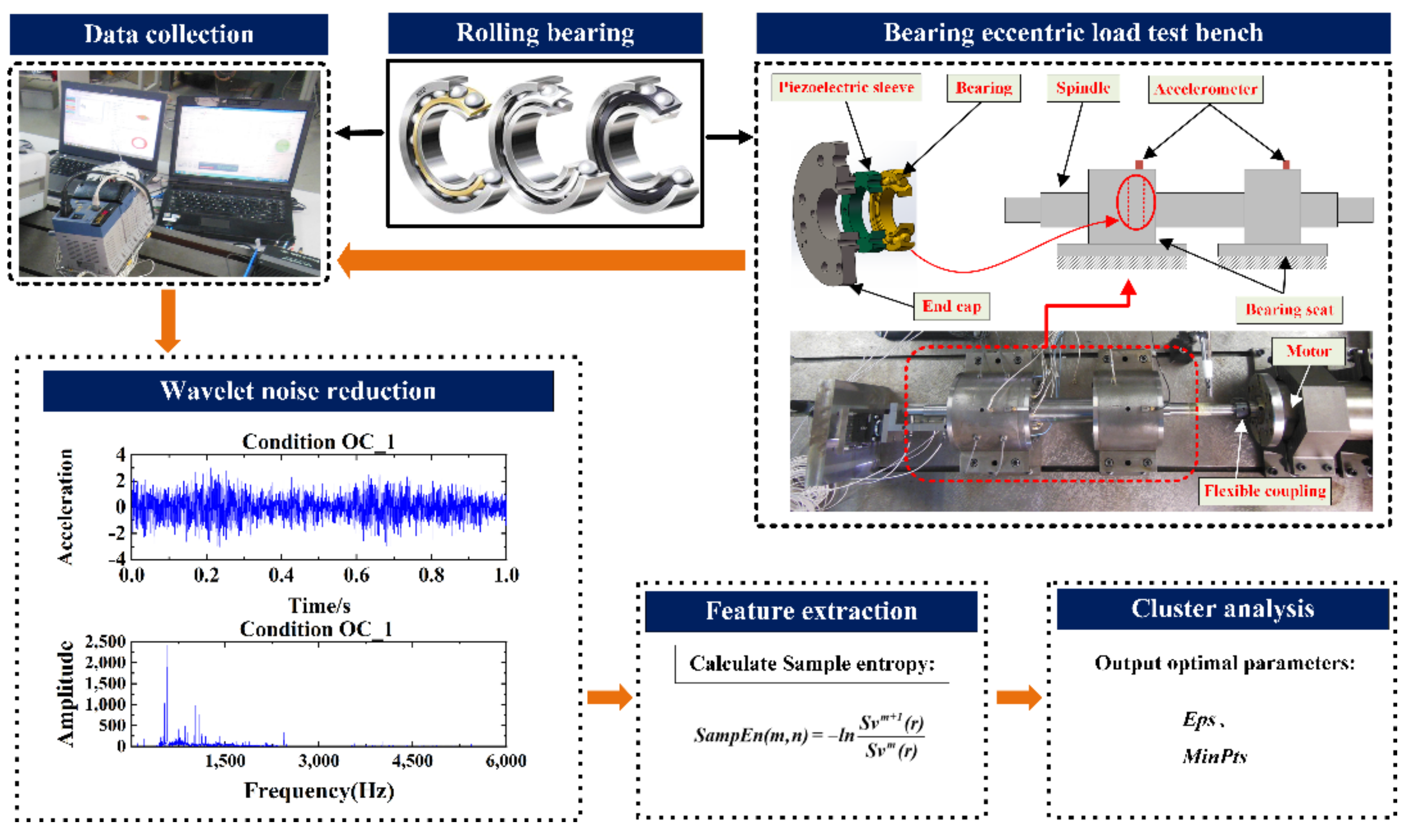
Using the state detection approach proposed in this paper, a flow chart for feature extraction and classification is shown in Figure 3.
  • It was built to collect vibration signals from rolling bearings under various deflection conditions.
  • Wavelet noise reduction is used to preprocess the original vibration signal before extracting kurtosis and sample entropy eigenvalues and building the Eigenvector dataset from the original vibration signal.
  • IDBSCAN clustering analyses are parameter-seeking, with the optimal parameters MinPts and Eps selected to utilize in the clustering analysis in the final monitoring results.

3. Algorithm Verification Based on IMS Bearing Test Bench

3.1. Data Collection

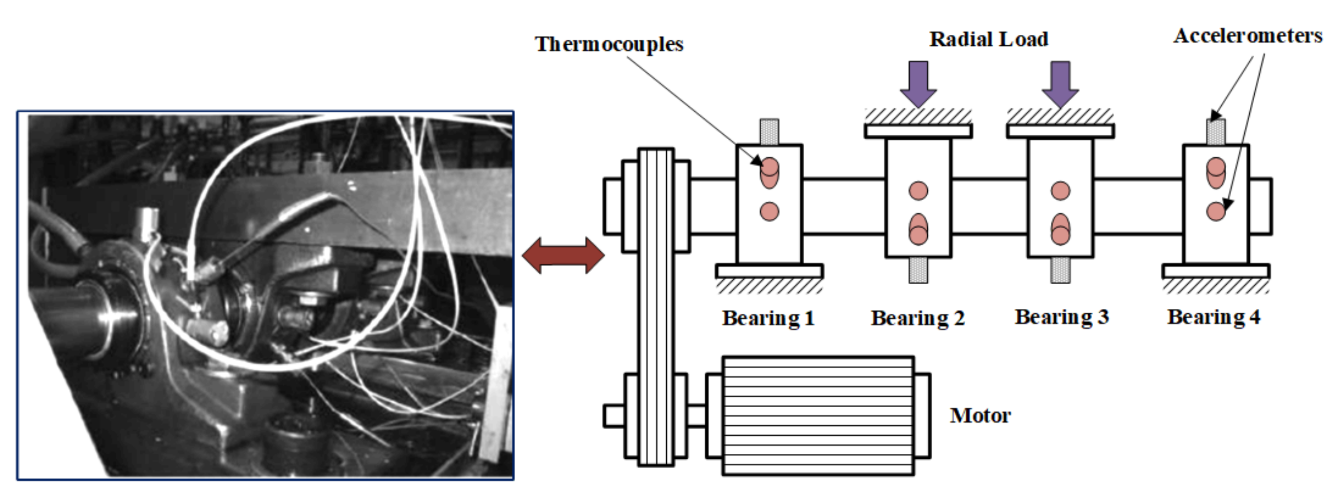
To validate the approach described in this paper’s practicality and accuracy, experimental validation of the bearing’s vibration state for each failure mode was performed. Using a double row bearing as an example, failure data was gathered from the University of Cincinnati’s Intelligent Maintenance System (IMS) bearing testing bench; the test bench’s exact structural components are depicted in Figure 4. A motor, four bearings, accelerometers, and other components comprise the bench. The bearing is a Rexnord ZA−2115 double row bearing with a sampling rate of 20 kHz, a sampling period of 1 s per sample, and a speed of 2000 r/min. Three data sets were obtained throughout the operating process, with bearing 3 in data set 1 exhibiting an inner ring crack, bearing 4 exhibiting a ball crack, and bearing 1 exhibiting a normal bearing; bearing 3 in data set 3 exhibiting an outer ring crack. The data collected in this article is representative of four distinct operating conditions: normal bearing operation, inner ring failure, rolling element failure, and outer ring failure. The sorts of defects that can occur during bearing operation are listed in Table 1.

3.2. Feature Extraction

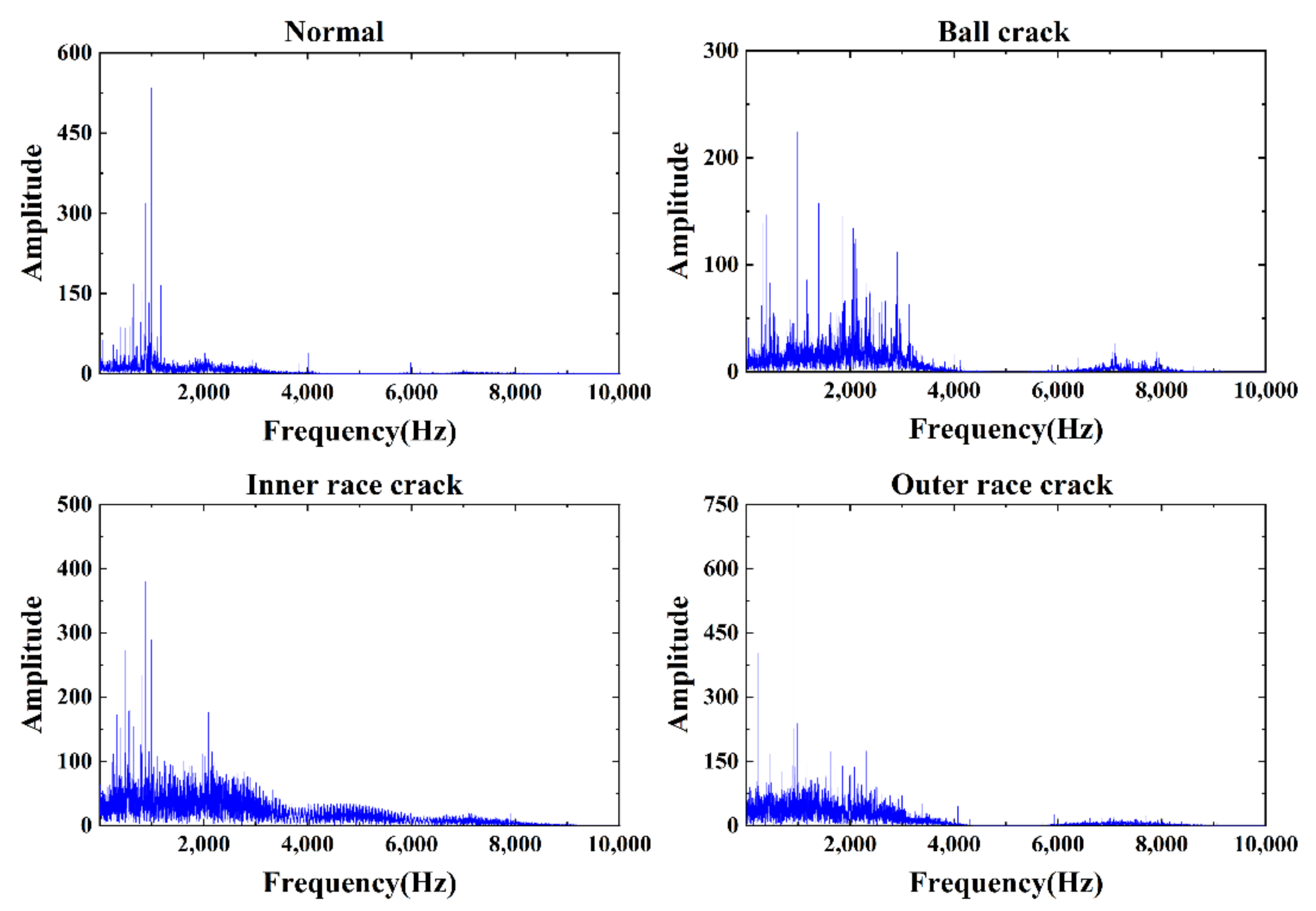
For each condition, the vibration data is retrieved within 1 s and examined in the temporal and frequency domains. In order to improve discrimination, the time domain signal was first subjected to the wavelet transform for noise reduction, and the result of the third layer wavelet transform was used to represent the vibration signal (Figure 5 and Figure 6). When a bearing has a ball crack, an inner ring crack and an outer ring break can be seen in these waveforms in time and frequency. Because the bearing rotates at a specific frequency, the amplitude difference seen in the graph in the low frequency region is less pronounced. However, the amplitude difference in the high frequency band appears to be larger, and the distribution is extremely intense due to the different types of faults. This paper uses a feature extraction method based on kurtosis and sample entropy to process the vibration signal after noise reduction in order to better distinguish the bearing crack type because it is difficult to distinguish the rolling bearing working state from time and frequency domain waveforms.
As a starting point, 163,800 data points were collected on the operational status of each bearing and averaged by 5120 data points per group to form 32 sets of sample data. Under the four operating circumstances, the 128 sets of sample data were then retrieved in the time domain for the kurtosis value and in the frequency domain for the entropy value. Finally, a two-dimensional feature vector with a length of 128 was generated. In order to illustrate that the feature calculation method of kurtosis and sample entropy is more suitable for the research content of this paper, the calculation methods of margin index, impulse index, and approximate entropy mentioned in the literature [37] were selected to compare with the feature calculation method of this paper. Figure 7 shows the characteristic distribution of each operating state of the bearing in five ways: Figure 7a shows the kurtosis distribution, Figure 7b shows the sample entropy distribution in the frequency domain, Figure 7c shows the margin index distribution, Figure 7d shows the impulse index distribution, and Figure 7e shows the approximate entropy distribution in the frequency domain. It can be seen that the margin index, impulse index, and approximate entropy in the four states all have poor coincidence. Among them, the margin index and impulse index in the outer ring fault mode have a large variation between sample groups. Although the approximate entropy between sample groups has a small change in amplitude, the approximate entropy in the inner ring fault and rolling element fault modes basically coincide, the discrimination is low. Therefore, this paper selects the kurtosis and the frequency domain sample entropy as the characteristic indicators of the condition monitoring, which provides a reference for the subsequent monitoring of the bearing unbalance condition.

3.3. Cluster Analysis

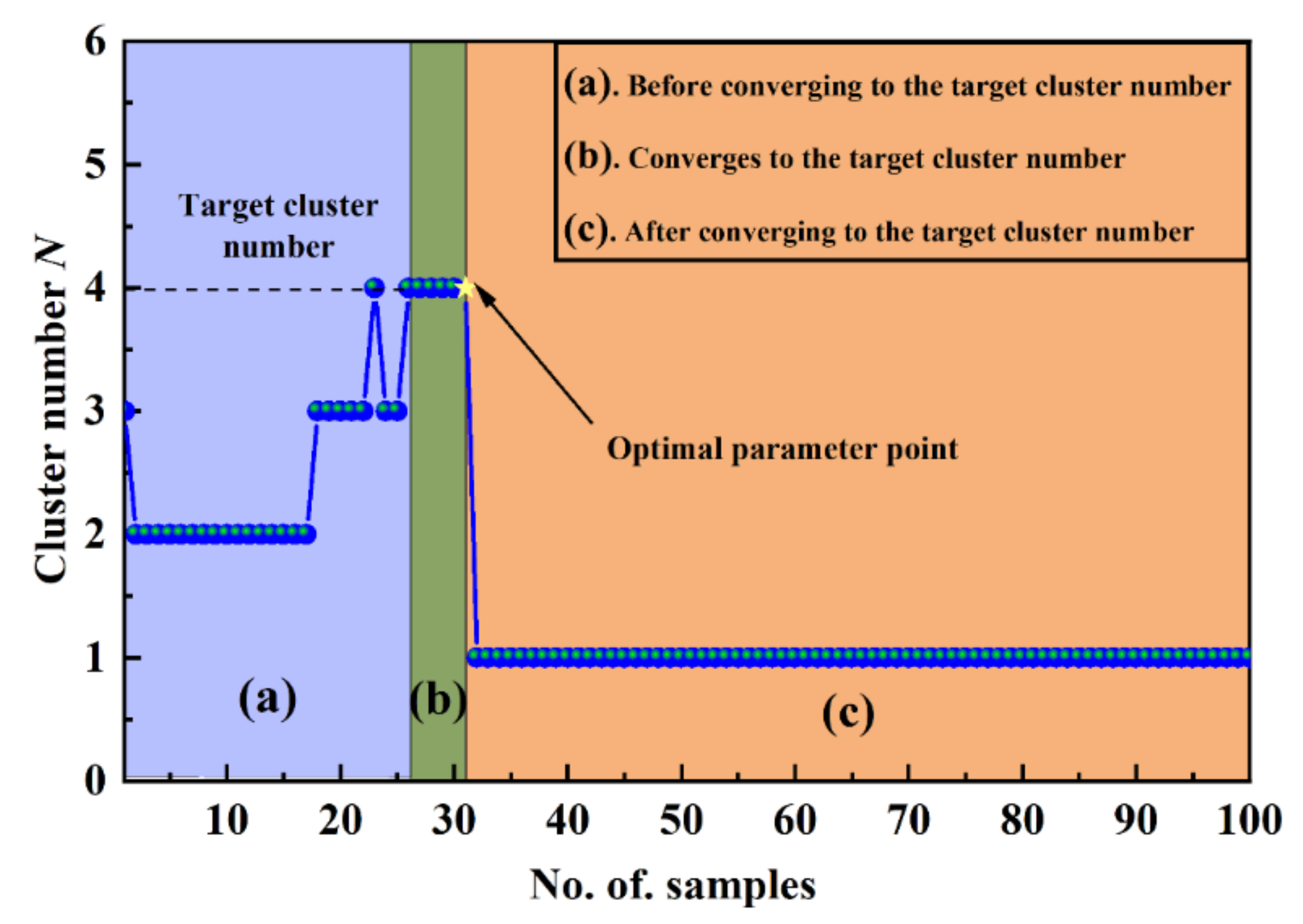
The feature vectors from Section 3.2 are used to build the data set Y ( E n t r o p y , k u r t o s i s ) , and the IDBSCAN algorithm from Section 2.2 is used to identify the parameters of the features, resulting in a list of Eps, MinPts variables. Finally, the number of clusters corresponding to each set of parameters is estimated. Figure 8 shows the relationship between the number of clusters and the number of samples, with the three intervals (a), (b), and (c) indicating convergence before, convergence to, and convergence after the target number of clusters, respectively.
As the number of samples K increases, the value of N fluctuates until it reaches the desired number of clusters. At K = 22, the target cluster number is attained for the first time, but the number of clusters rapidly varies until it stabilizes and converges to the target cluster number at K = 26. Then, at K = 31, a mutation occurs, and the value of N converges to one as K increases, indicating that all feature values fall into a cluster of 1, however this does not conform to our target value selection restrictions. Therefore, when K = 31, the ideal parameters are determined, and the list of Eps and MinPts parameters indicates that the optimal parameters are Eps = 0.1717 and MinPts = 28, respectively.
Clustering analysis was performed using the ideal parameters Eps = 0.1717 and MinPts = 28 as well as two-dimensional feature vector of kurtosis and sample entropy. The number of samples is used as a third dimension in this study to better understand the clustering effect. IMS load-bearing state feature clustering is displayed in Figure 9 (below). The clustering effect can be seen in the figure under four conditions: normal bearing operation, inner ring failure, rolling element failure, and outer ring failure. Since the greater shocks they produce have a high kurtosis and entropy value, failures of the outer and inner rings are more common. The 99.2 percent accurate state feature distribution diagram produced by this method only had one missing feature point. As shown in this research, data from the IMS bearing test stand paired with the condition monitoring methods may be used to accurately characterize the operating conditions of bearings using kurtosis-based, frequency domain sample entropy characterization, and improved DBSCAN clustering analysis.

4. Algorithm Verification Based on Unbalanced Bearing’s Load Test Bench

4.1. Data Collection

An unbalanced bearing load test bench was developed and constructed in this manuscript to further examine the monitoring function of the suggested technique during biased bearing operation, as seen in Figure 10. The test bench primarily consists of a motor, a precision spindle, a rolling bearing, and an acceleration sensor, with the electric spindle reaching a maximum speed of 10,000 r/min. The mechanical spindle is coupled to the electric spindle by a flexible coupling, and the motor operation is controlled via the servo control system.
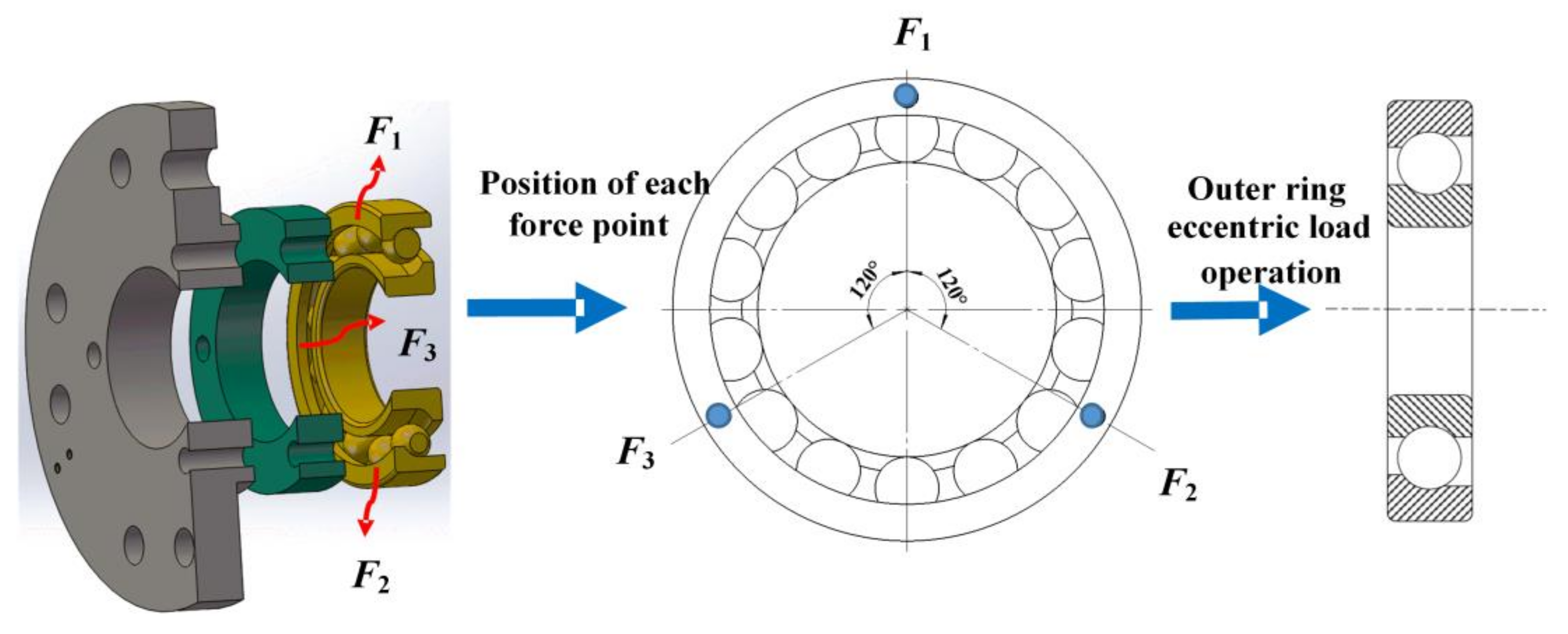
Four NSK7014C angular contact ball bearings were employed in this test bench. Figure 11 illustrates the bearing structure loaded schematic diagram, where F1, F2, and F3 are loaded on the bearing at 120°, respectively, and the bearing bias running state is defined by setting different sizes of preload; the bearings are mounted back-to-back, the fixed speed is 4000 r/min, the sampling frequency is 8192 Hz, and the sampling length is 512. Table 2 shows the bearing parameters.
This manuscript defines six bearing operating states for light (OC_1, OC_01), medium (OC_2 OC_02), and heavy load circumstances (OC_3, OC_03), where (OC_1, OC_2, OC_3) denotes operation with an imbalanced load and (OC 01, OC 02, OC 03) denotes operation with an even load. Table 3 summarizes the forces present in each condition.

4.2. Feature Extraction

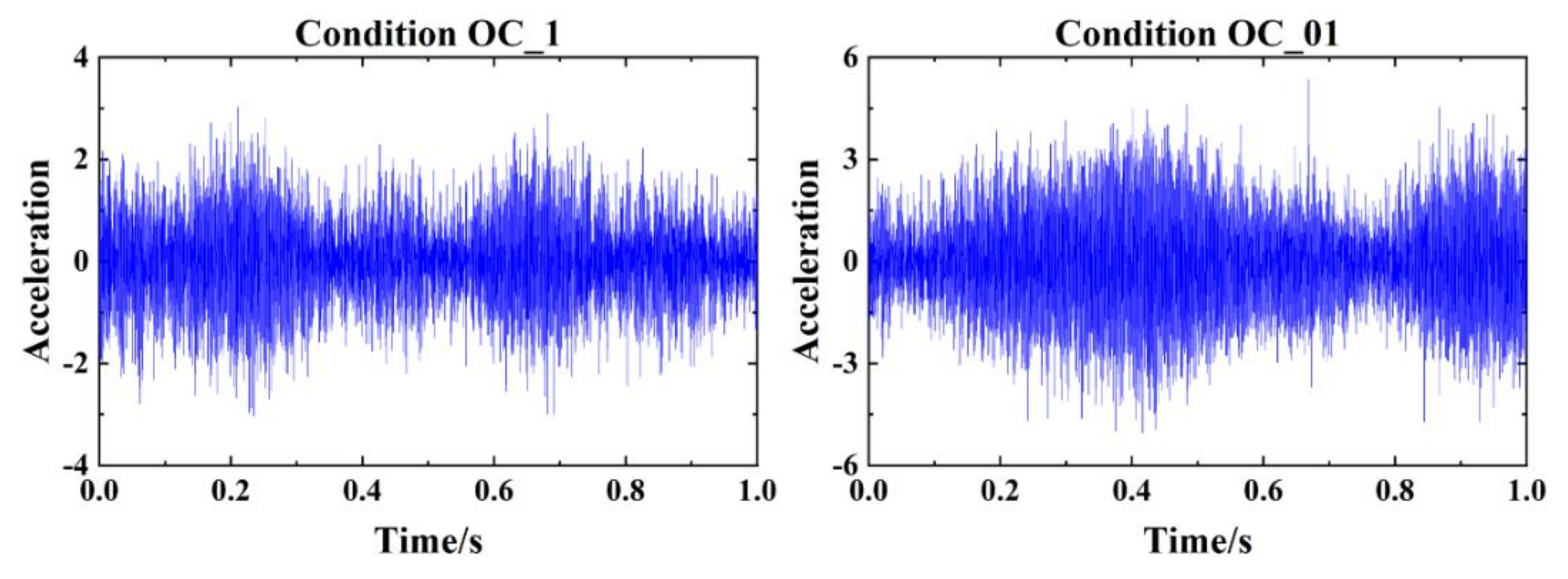
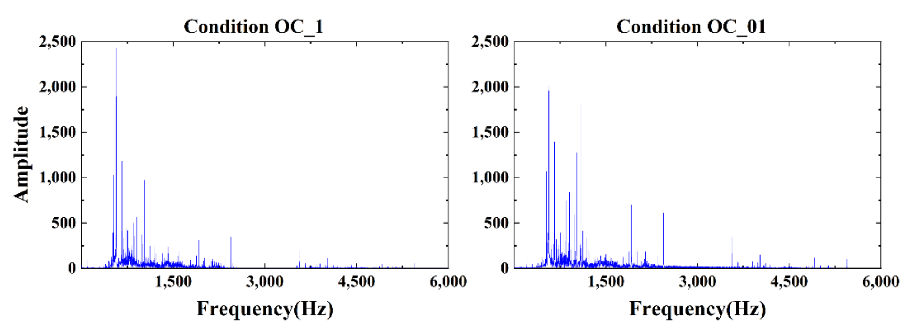
Similarly, vibration signals within one second were extracted for analysis, wavelet noise reduction was performed to the extracted vibration signals, and the resulting time and frequency domain waveforms were shown. The time domain waveform of the bearing under load after wavelet noise reduction is shown in Figure 12. As seen in the picture, the amplitude of the periodic variation in operating state OC_1 is greater than that in state OC_01, while the amplitude of the acceleration is smaller. The time domain waveform reveals the change in operational condition intuitively. The frequency domain waveform of the bearing loaded after wavelet noise reduction is shown in Figure 13. As shown in the figure, the low frequency band part has a relatively small difference in amplitude because the bearing has a fixed rotation frequency, but the high frequency band has a noticeable difference in amplitude because the bearing is loaded differently. In order to better distinguish the bearing crack type, the algorithm developed in this paper is used to analyze and process the data.
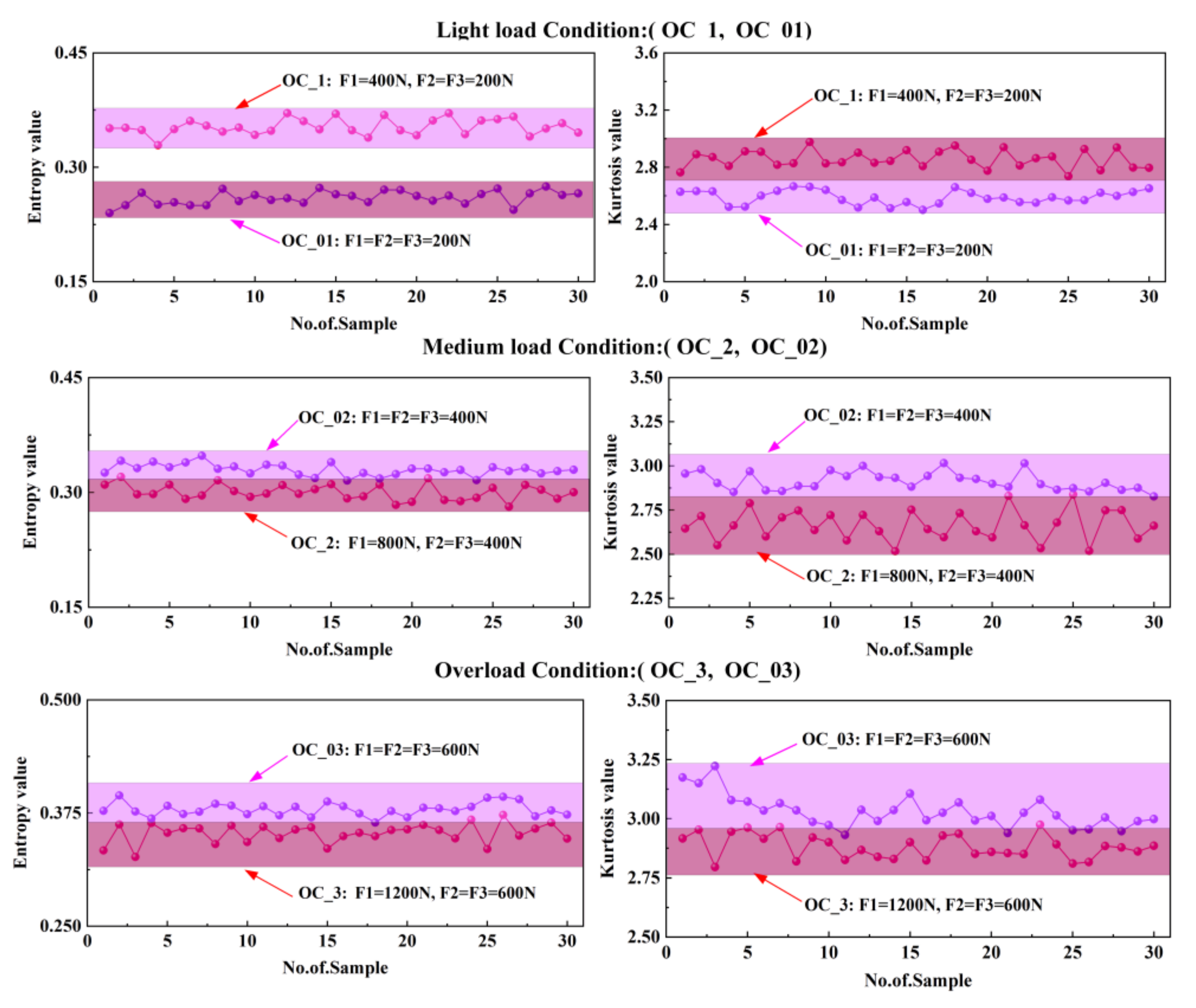
During data collection, the collection time of each state of the bearing is set to 30 s, a total of 245,760 data points are obtained, and then the data points are divided by the equal time series method to obtain a multi-dimensional array of Y8192 × 30, where 8192 represents a single the length of the time series, and 30 represents the number of time series. Next, kurtosis and sample entropy values were extracted from 180 sets of sample data under the six working conditions, yielding a two-dimensional feature vector of length 180. The extracted feature data are classified into three operating conditions: light load (OC_1, OC_01), medium load (OC_2, OC_02), and heavy load (OC_3, OC_03). The kurtosis and frequency domain sample entropy values of the bearings’ unbalanced load and uniform-load operating states are calculated using the method proposed in this paper. The typical distribution of the bearing under working conditions is depicted in Figure 14 for the operating conditions (OC_1, OC_01), (OC_2, OC_02), and (OC_3, OC_03). The frequency domain sample entropy and kurtosis values of the operating state of unbalanced load (OC_01) are greater and more distinct than those of the uniform loaded state (OC_1) under light load conditions. The eigenvalues of the states under medium and heavy load conditions are less distinct, and the eigenvalues of the uniform loaded state are greater. To improve the identification of the state distribution under each operating situation, the feature vectors are processed and evaluated using an improved DBSCAN clustering algorithm.

4.3. Cluster Analysis

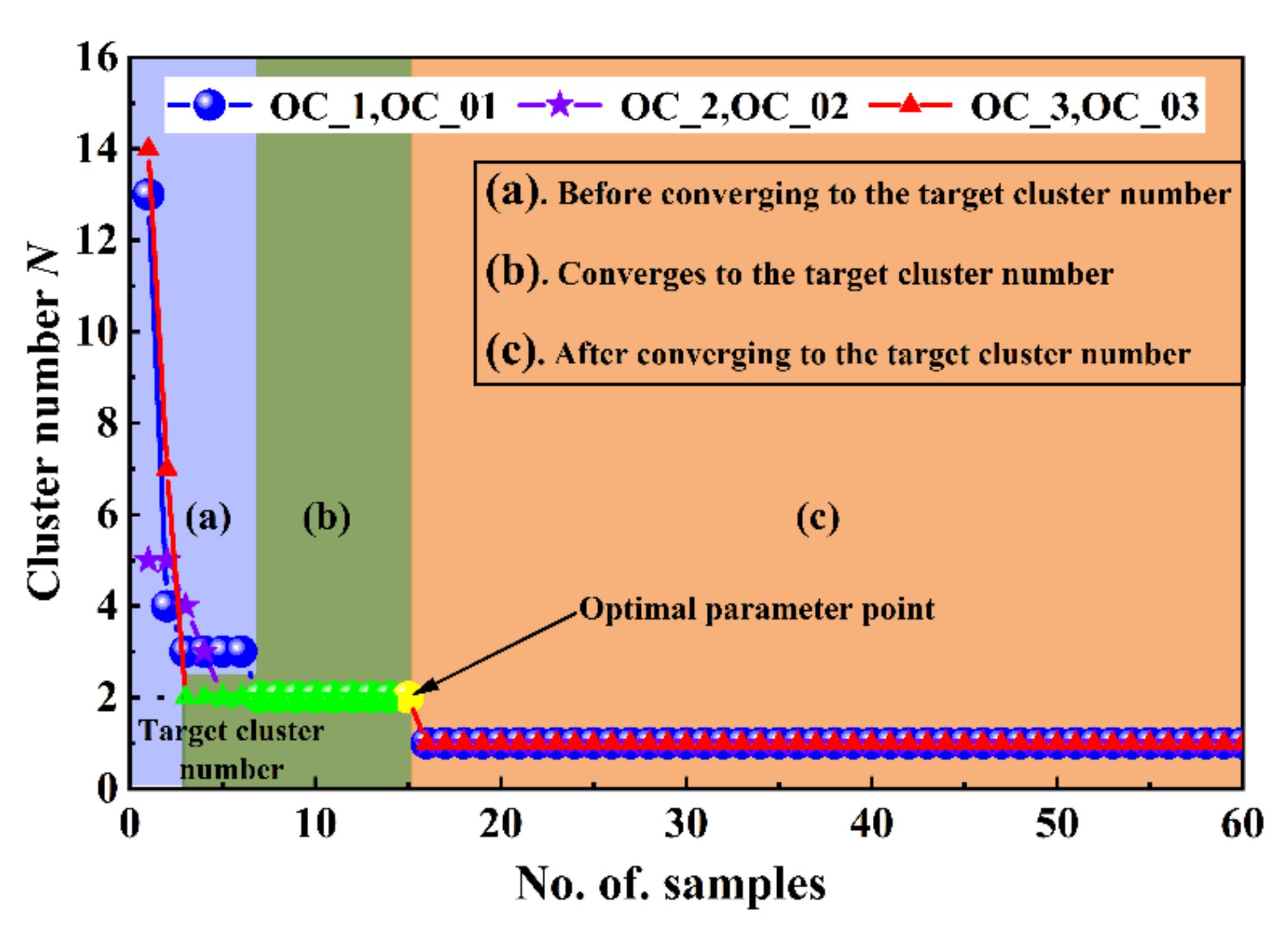
Construct a data collection of light load, medium load, and overload circumstances using the feature vectors in Section 4.2, including: Y E n t r o p y , K u r t o s i s ( O C _ 1 , O C _ 1 ) , Y E n t r o p y , K u r t o s i s ( O C _ 2 , O C _ 2 ) and Y E n t r o p y , K u r t o s i s ( O C _ 3 , O C _ 3 ) . The IDBSCAN algorithm described in Section 2.2 is used to calculate the optimal feature parameters. Firstly, the Eps and MinPts parameter lists for each working condition are obtained by training the data set, then the feature vectors are clustered according to the values of the parameter lists from smallest to largest, and the change in the number of clusters formed by each group of parameters is observed. When the number of clusters converges to the target number of clusters, the parameter corresponding to that position is selected as the optimal parameter for the cluster analysis. Figure 15 shows the finding curve of clustering parameter for each loading condition. The curve (a), (b), and (c) in Figure 15 represents the three stages of the optimization curve: (a), (b), and (c) represent the convergence before the target number of clusters, the convergence on the target number of clusters, and after the convergence on the target number of clusters, and after the convergence on the target number of clusters, respectively. Where (a) indicates the number of clusters from the minimum threshold and kernel radius to calculate the clustering effect, with the value of N getting closer to the target as the parameter values continue to increase, (b) indicates when N has just reached the target number of clusters, with increasing parameter values and the number of clusters remaining constant until the next mutation is generated. At this point, the number of samples K before the mutation is the definitive position for our search for the optimal parameter; (c) indicates that the condition that the number of clusters in the feature set is 1, deviating from the rule for which we are searching for the optimum. The figure shows that the target is 2 for all three loaded conditions. The number of clusters changes and gradually approaches the target as the number of samples increases, for which the optimal parameter determination position K is the same for all three conditions. Finally, based on the value of K, the related parameters Eps and MinPts were determined, as shown in Table 4.
Cluster analysis of the feature vectors for each operating condition according to the parameters Eps and MinPts in Table 4. Figure 16 shows the clustering parameter optimization curves for different loading conditions, where Figure 16a–c illustrate the distribution of characteristics under light load, medium load, and overload conditions, respectively. The categorization effect is immediately apparent, with an accuracy of 98.4%, and only one feature point was not recognized under light and medium load circumstances. Two feature points were not detected with an accuracy of 96.7% under overload conditions. Thus, by constructing an unbalanced bearing load test bench and combining it with the suggested condition monitoring approach in this paper, the research demonstrates that this method is capable of efficiently distinguishing the distribution of bearing load conditions under different preload.

5. Conclusions

The purpose of this research is to propose an IDBSCAN spindle condition monitoring approach based on kurtosis and sample entropy for more accurate identification of the spindle operating status and intelligent spindle condition assessment. The approach begins by performing wavelet noise reduction on the original state data and then segmenting it into numerous groups, collecting the kurtosis and frequency domain sample entropy values for each group to generate a two-dimensional feature vector. The IDBSCAN clustering algorithm is then used to discover the best parameters Eps and MinPts using the two-dimensional feature vector. Finally, the ideal parameters are used to monitor the feature vectors of various state categories. The algorithm was validated using data from the University of Cincinnati’s IMS bearing test rig, which was then confirmed using the test bench for bearing operation under varying preloads. The following conclusions have been drawn:
  • Weak bearing characteristics may be effectively extracted using the proposed kurtosis and frequency domain sample entropy-based feature extraction method.
  • An updated DBSCAN method enables automatic cluster analysis by determining the optimal values of the Eps and MinPts parameters, as well as the position of the optimal parameters, using a more precise optimization strategy.
  • Using the condition monitoring approach proposed in the paper, the experimental results reveal that both bearings in fault conditions and bearings under varying loading conditions can be identified, and the condition detection rate is extremely high, reaching 96% in all cases.
  • Although this work demonstrates that the operating condition of a bearing may be recognized under both unbalanced and uniform load situations, the recognition effect of operating the bearing under diverse load conditions is not clearly demonstrated.

Author Contributions

Conceptualization, Y.Z. and Y.L.; methodology, Y.L.; validation, Y.Z., Y.L. and L.K.; formal analysis, Q.N. and Y.B.; investigation, L.K. and Q.N.; data curation, Y.L.; writing—original draft preparation, Y.L.; writing—review and editing, Y.Z.; visualization, Y.L.; supervision, Y.B.; project administration, Q.N.; and funding acquisition, Y.Z. All authors have read and agreed to the published version of the manuscript.

Funding

This research was supported by the National Natural Science Foundation of China (52005405) and Postdoctoral Science Foundation of China (2019M660075XB).

Institutional Review Board Statement

Not applicable.

Informed Consent Statement

Not applicable.

Data Availability Statement

Detailed data are contained within the article.

Acknowledgments

This research was supported by the National Natural Science Foundation of China (52005405) and Postdoctoral Science Foundation of China (2019M660075XB).

Conflicts of Interest

The author(s) declared no potential conflict of interest with respect to the research, authorship, and/or publication of this article.

References

  1. Ma, J.; Li, Z.; Li, C.; Zhan, L.; Zhang, G. Rolling Bearing crack Diagnosis Based on Refined Composite Multi-Scale Approximate Entropy and Optimized Probabilistic Neural Network. Entropy 2021, 23, 259. [Google Scholar] [CrossRef] [PubMed]
  2. Gu, R.; Chen, J.; Hong, R.; Wang, H.; Wu, W. Incipient fault diagnosis of rolling bearings based on adaptive vibrational mode decomposition and Teager energy operator. Measurement 2020, 149, 106941. [Google Scholar] [CrossRef]
  3. Liu, H.; Zhang, Y.; Li, C.; Li, Z. Nonlinear dynamic analysis of CNC lathe spindle-bearing system considering thermal effect. Nonlinear Dyn. 2021, 105, 131–166. [Google Scholar] [CrossRef]
  4. Tian, S.; Zhao, X.; Dong, S. Dynamic support stiffness of motorized spindle bearings under high-speed rotation. Int. J. Adv. Manuf. Technol. 2021, 117, 2359–2367. [Google Scholar] [CrossRef]
  5. Zhao, H.; Yang, Z.; Chen, C.; Tian, H.; Chen, L.; Ying, J.; Jia, X. Development of Reliability Test System Based on Working Principle and Fault Analysis of Motorized Spindle. In Proceedings of the 2018 3rd International Conference on System Reliability and Safety (ICSRS), Barcelona, Spain, 23–25 November 2018; pp. 299–307. [Google Scholar]
  6. Yi, J.; Pang, B.; Liu, H.; Wang, F.; Ji, B.; Jing, M. Influence of Misalignment on Nonlinear Dynamic Characteristics for Matched Bearings-Rotor System. Proc. Inst. Mech. Eng. Part K J. Multi-Body Dyn. 2014, 228, 172–181. [Google Scholar] [CrossRef]
  7. Lin, J.L.; Liu, J.Y.C.; Li, C.W.; Tsai, L.F.; Chung, H.Y. Motor shaft misalignment detection using multiscale entropy with wavelet denoising. Expert Syst. Appl. 2010, 37, 7200–7204. [Google Scholar] [CrossRef]
  8. Xing, Y.; Xu, H.; Pei, S.; Zhang, X.; Chang, W. Mechanical Analysis of Spherical Roller Bearings Due to Misalignments between Inner and Outer Rings. Proc. Inst. Mech. Eng. Part C J. Mech. Eng. Sci. 2016, 231, 3250–3262. [Google Scholar] [CrossRef]
  9. Li, L.; Zhang, D.; Xie, Y. Effect of misalignment on the dynamic characteristic of MEMS gas bearing considering rarefaction effect. Tribol. Int. 2019, 139, 22–35. [Google Scholar] [CrossRef]
  10. Tong, V.C.; Kwon, S.W.; Hong, S.W. Fatigue Life of Cylindrical Roller Bearings. Proc. Inst. Mech. Eng. Part J J. Eng. Tribol. 2017, 231, 623–636. [Google Scholar] [CrossRef]
  11. Li, Z.; Li, J.; Li, M. Nonlinear Dynamics of Unsymmetrical Rotor-Bearing System with Fault of Parallel Misalignment. Adv. Mech. Eng. 2018, 10, 1687814018772908. [Google Scholar] [CrossRef] [Green Version]
  12. Xie, Z.; Shen, N.; Zhu, W.; Tian, W.; Hao, L. Theoretical and experimental investigation on the influences of misalignment on the lubrication performances and lubrication regimes transition of water lubricated bearing. Mech. Syst. Signal Process. 2021, 149, 107211. [Google Scholar] [CrossRef]
  13. Rai, A.; Upadhyay, S.H. A review on signal processing techniques utilized in the fault diagnosis of rolling element bearings. Tribol. Int. 2016, 96, 289–306. [Google Scholar] [CrossRef]
  14. Li, H.; Liu, T.; Wu, X.; Chen, Q. Application of EEMD and improved frequency band entropy in bearing crack feature extraction. ISA Trans. 2019, 88, 170–185. [Google Scholar] [CrossRef] [PubMed]
  15. Xu, Z.; Tang, G.; He, M. Peak-Based Mode Decomposition for Weak Fault Feature Enhancement and Detection of Rolling Element Bearing. Shock. Vib. 2020, 2020, 8901794. [Google Scholar] [CrossRef]
  16. Ding, C.; Feng, F.; Zhang, B.; Wu, S. Improved multi-scale symbolic dynamics information entropy and its application in feature extraction of planetary gearboxes. Vib. Shock. 2020, 39, 97–102. [Google Scholar]
  17. Castellani, F.; Garibaldi, L.; Daga, A.P.; Astolfi, D.; Natili, F. Diagnosis of Faulty Wind Turbine Bearings Using Tower Vibration Measurements. Energies 2020, 13, 1474. [Google Scholar] [CrossRef] [Green Version]
  18. Chen, B.; Yan, Z.; Chen, W. Defect Detection for Wheel-Bearings with Time-Spectral Kurtosis and Entropy. Entropy 2014, 16, 607–626. [Google Scholar] [CrossRef] [Green Version]
  19. Rohani Bastami, A.; Bashari, A. Rolling element bearing diagnosis using spectral kurtosis based on optimized impulse response wavelet. J. Vib. Control 2020, 26, 175–185. [Google Scholar] [CrossRef]
  20. Tian, J.; Morillo, C.; Azarian, M.H.; Pecht, M. Motor Bearing crack Detection Using Spectral Kurtosis-Based Feature Extraction Coupled With K-Nearest Neighbor Distance Analysis. IEEE Trans. Ind. Electron. 2016, 63, 1793–1803. [Google Scholar] [CrossRef]
  21. Zhong, J.; Wang, D.; Guo, J.; Cabrera, D.; Li, C. Theoretical Investigations on Kurtosis and Entropy and Their Improvements for System Health Monitoring. IEEE Trans. Instrum. Meas. 2021, 70, 3503710. [Google Scholar] [CrossRef]
  22. Shang, Y.; Lu, G.; Kang, Y.; Zhou, Z.; Duan, B.; Zhang, C. A multi-fault diagnosis method based on modified Sample Entropy for lithium-ion battery strings. J. Power Sources 2020, 446, 227275. [Google Scholar] [CrossRef]
  23. Lin, T.-K.; Chien, Y.-H. Performance Evaluation of an Entropy-Based Structural Health Monitoring System Utilizing Composite Multiscale Cross-Sample Entropy. Entropy 2019, 21, 41. [Google Scholar] [CrossRef] [PubMed] [Green Version]
  24. Sandoval, D.; Leturiondo, U.; Vidal, Y.; Pozo, F. Entropy Indicators: An Approach for Low-Speed Bearing Diagnosis. Sensors 2021, 21, 849. [Google Scholar] [CrossRef] [PubMed]
  25. Delgado-Bonal, A.; Marshak, A. Approximate Entropy and Sample Entropy: A Comprehensive Tutorial. Entropy 2019, 21, 541. [Google Scholar] [CrossRef] [PubMed] [Green Version]
  26. Han, M.; Pan, J. A fault diagnosis method combined with LMD, sample entropy and energy ratio for roller bearings. Measurement 2015, 76, 7–19. [Google Scholar] [CrossRef]
  27. Wang, Z.; Yao, L.; Cai, Y. Rolling bearing crack diagnosis using generalized refined composite multiscale sample entropy and optimized support vector machine. Measurement 2020, 156, 107574. [Google Scholar] [CrossRef]
  28. Mouchaweh, M.S. Advanced Pattern Recognition method for the Monitoring of Dynamic Systems. IFAC Proc. Vol. 2009, 42, 510–515. [Google Scholar] [CrossRef]
  29. Kankar, P.K.; Sharma, S.C.; Harsha, S.P. Fault diagnosis of ball bearings using machine learning methods. Expert Syst. Appl. 2011, 38, 1876–1886. [Google Scholar] [CrossRef]
  30. Dong, L.; Shi, R.; Zeng, Z. Fault diagnosis of hoist spindle system based on complex network clustering. Vib. Test Diagn. 2016, 36, 688–693, 809. [Google Scholar]
  31. Li, C.; Cabrera, D.; De Oliveira, J.V.; Sanchez, R.V.; Cerrada, M.; Zurita, G. Extracting repetitive transients for rotating machinery diagnosis using multiscale clustered grey infogram. Mech. Syst. Signal Process. 2016, 76–77, 157–173. [Google Scholar] [CrossRef]
  32. Shi, J.; Deng, Y.; Wang, Z.; Guo, X. An adaptive new state recognition method based on density peak clustering and voting probabilistic neural network. Appl. Soft Comput. 2020, 97, 1876–1886. [Google Scholar] [CrossRef]
  33. Du, M.; Ding, S.; Jia, H. Study on density peaks clustering based on k-nearest neighbors and principal component analysis. Knowl. -Based Syst. 2016, 99, 135–145. [Google Scholar] [CrossRef]
  34. Kerroumi, S.; Rasolofondraibe, L.; Chiementin, X. Dynamic Pattern Recognition Method for Bearing Monitoring. Proceedings of ISMA 2014; Katholieke Universiteit Leuven: Leuven, Belgium, 2014; pp. 2809–2820. [Google Scholar]
  35. Li, H.; Wang, W.; Huang, P.; Li, Q. Fault diagnosis of rolling bearing using symmetrized dot pattern and density-based clustering. Measurement 2020, 152, 107293. [Google Scholar] [CrossRef]
  36. Li, W.; Yan, S.; Jiang, Y.; Zhang, S.; Wang, C. Research on adaptively determining DBSCAN algorithm parameters. Comput. Eng. Appl. 2019, 55, 1–7. [Google Scholar]
  37. Caesarendra, W.; Tjahjowidodo, T. A Review of Feature Extraction Methods in Vibration-Based Condition Monitoring and Its Application for Degradation Trend Estimation of Low-Speed Slew Bearing. Machines 2017, 5, 21. [Google Scholar] [CrossRef]
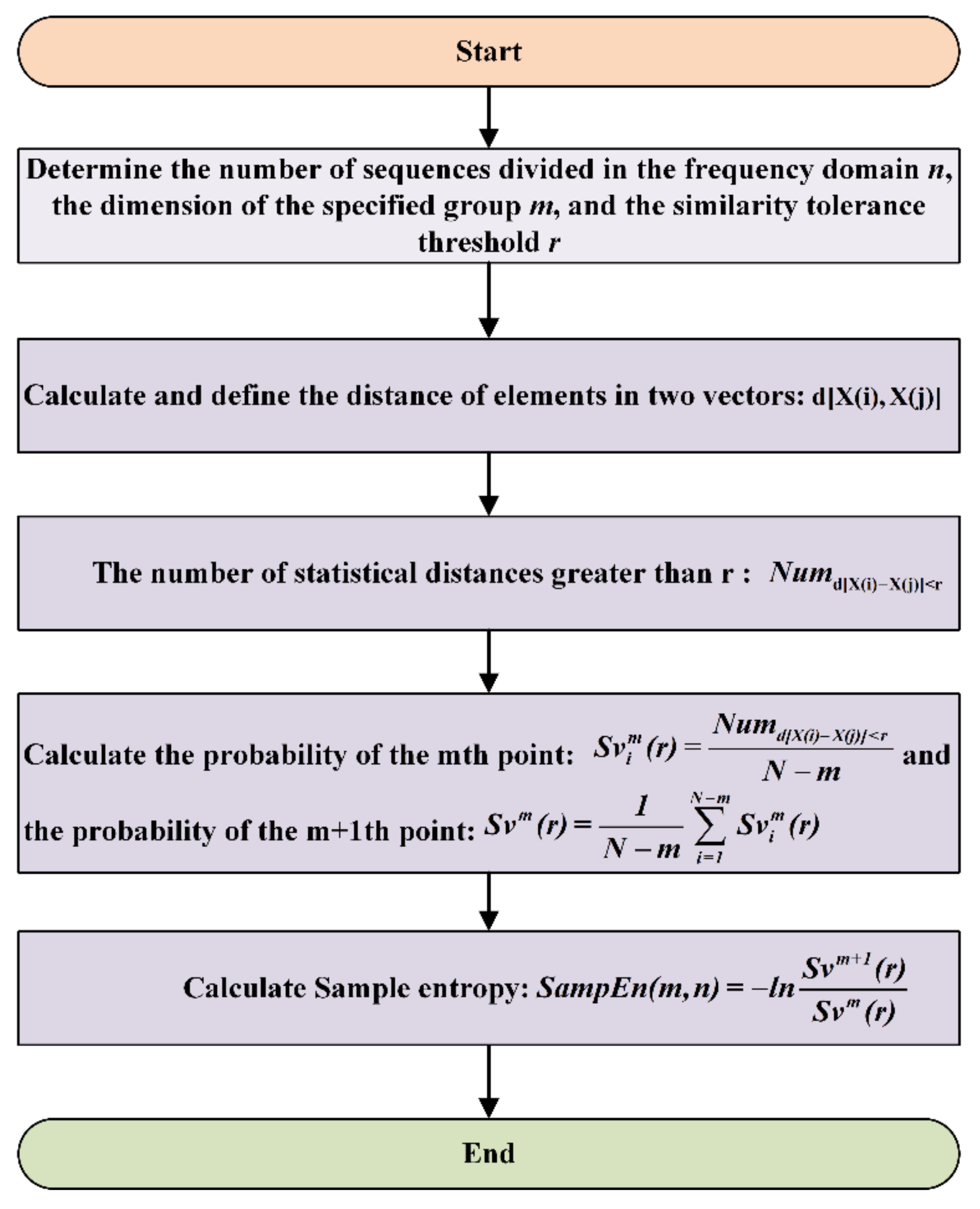
Figure 1. Frequency domain sample entropy calculation flow diagram.
Machines 10 00363 g001
Figure 2. Improved DBSCAN clustering algorithm flow diagram.
Machines 10 00363 g002
Figure 3. Feature extraction and state classification flow chart.
Machines 10 00363 g003
Figure 4. Bearing test bench and structure diagram.
Machines 10 00363 g004
Figure 5. Wavelet de-noising time domain waveform of IMS bearing test raw data.
Machines 10 00363 g005
Figure 6. Wavelet de-noising frequency domain waveforms of IMS bearing test raw data.
Machines 10 00363 g006
Figure 7. Feature distribution diagram of IMS bearing under various working conditions: (a) Sample entropy value, (b) Kurtosis value, (c) Margin value, (d) Impulse value, (e) AE value.
Machines 10 00363 g007
Figure 8. The relationship between the number of clusters and the value of the sample.
Machines 10 00363 g008
Figure 9. IMS bearing state feature clustering effect diagram.
Machines 10 00363 g009
Figure 10. Bearing non-uniform preload test bench.
Machines 10 00363 g010
Figure 11. Schematic diagram of bearing structure loading.
Machines 10 00363 g011
Figure 12. Time domain waveform diagram of bearing load after wavelet noise reduction.
Machines 10 00363 g012
Figure 13. Frequency domain waveform diagram of bearing load after wavelet noise reduction.
Machines 10 00363 g013
Figure 14. The characteristic distribution map of the bearing running under different load conditions.
Machines 10 00363 g014
Figure 15. Clustering parameter optimization curve diagram under various loading conditions.
Machines 10 00363 g015
Figure 16. The optimal clustering results under each load condition: (a) light load (OC_1, OC_01), (b) medium load (OC_2, OC_02), overload (c) (OC_3, OC_03).
Machines 10 00363 g016
Table 1. Bearing failure category table.
Data Set NumberFault TypeSampling Length
Data set 1-bearing 1Normal81,920
Data set 1-bearing 3Inner ring crack81,920
Data set 1-bearing 4Boll crack81,920
Data set 3-bearing 3Outer ring crack81,920
Table 2. NSK7014C angular contact ball bearing parameters table.
Inner Ring
Diameter/mm
Outer Ring Diameter/mmThickness/mmDynamic Load/KNStatic Load/mm
70100204743
Table 3. Bearing loading conditions and operating conditions table.
Operational StateF1/NF2/NF3/N
OC_1400200200
OC_2800400400
OC_31200600600
OC_01200200200
OC_02400400400
OC_03600600600
Table 4. Cluster analysis optimal parameter table.
Loaded ConditionsEpsMinPts
(OC_1,OC_01)0.168217
(OC_2,OC_02)0.224116
(OC_3,OC_03)0.241217
Publisher’s Note: MDPI stays neutral with regard to jurisdictional claims in published maps and institutional affiliations.