Abstract
Transfer learning is a topic that has attracted attention for the intelligent fault diagnosis of bearings since it addresses bearing datasets that have different distributions. However, the traditional intelligent fault diagnosis methods based on transfer learning have the following two shortcomings. (1) The multi-mode structure characteristics of bearing datasets are neglected. (2) Some local regions of the bearing signals may not be suitable for transfer due to signal fluctuation. Therefore, a multi-domain weighted adversarial transfer network is proposed for the cross-domain intelligent fault diagnosis of bearings. In the proposed method, multi-domain adversarial and attention weighting modules are designed to consider bearing multi-mode structure characteristics and solve the influence of local non-transferability regions of signals, respectively. Two diagnosis cases are used to verify the proposed method. The results show that the proposed method is able to extract domain invariant features for different cross-domain diagnosis cases, and thus improves the accuracy of fault identification.
1. Introduction
Transfer learning aims to use the existing knowledge to solve related, but different, domain of problems, discarding the constraint that the training and testing sets of intelligent models must obey the same probability distribution [1,2,3]. According to this advantage, researchers have introduced it into the field of the intelligent fault diagnosis of bearings and have proposed several transfer intelligent fault diagnosis methods [4,5,6,7,8]. These methods regard different bearing datasets as different domains, and the fault knowledge learned from one dataset in the source domain can be applied to the other dataset in the target domain by using domain adaptation, which breaks the limitations of traditional intelligent fault diagnosis methods based on deep learning [9,10,11,12,13]. For example, Du et al. [14] presented a hybrid transfer method, which achieved the transfer of fault knowledge between different domains by the transfer component analysis method and the TrAdaBoost algorithm. Yang et al. [15] established a transfer fault diagnosis method based on a polynomial kernel-induced maximum mean discrepancy, which solved the problem of transfer fault diagnosis between different bearings. Guo et al. [16] proposed a deep transfer learning network based on a one-dimensional deep convolutional neural network. Zou et al. [17] established a novel transfer fault diagnosis for the fault diagnosis of bearings under different working conditions, which combined deep convolution Wasserstein adversarial networks and a novel variance constraint to achieve a higher fault diagnosis accuracy than the existing models.
The main goal of this paper is to improve the diagnosis accuracy of the transfer learning bearing fault diagnosis method. The traditional intelligent fault diagnosis method based on transfer learning has two disadvantages. On the one hand, the multi-mode structure characteristics of bearing datasets are neglected. On the other hand, some local regions of the bearing signals may not be suitable for transfer due to signal fluctuation. The existing intelligent diagnosis methods have not considered these characteristics in the process of domain adaptation, and just align the learned features by directly measuring the overall distributions of the source and target domains [18,19,20,21,22]. It may lead to a misalignment between the multi-mode structure bearing datasets [23]. In addition, some local regions of the signals in the bearing datasets may be coupled with useless interference information due to the influence of background noise in the collection, which makes those local regions of the signals unsuitable for transfer [24,25,26,27,28,29].
In order to solve the above shortcomings, this paper addresses the following two tasks: (1) to consider the multi-mode structure characteristics of bearing datasets and (2) to solve the influence of local non-transferable area of signals. Based on these two tasks, a multi-domain weighted adversarial transfer network (MWAT) is proposed for cross-domain intelligent fault diagnosis by considering the bearing multi-mode data structure and the local non-transferability of the bearing signals. In the proposed MWAT, firstly, the feature extraction module is designed based on a convolution neural network and non-local network. This module aims to map the bearing data to the high-dimensional feature space to extract high-dimensional feature information. Secondly, the multi-domain adversarial module is established by considering the multi-mode structure characteristics of the bearing data. By capturing such multi-mode structure information, this module achieves the adversarial transfer training for the different health states of the data by using different channels. Thirdly, the attention weighted module is designed by considering the existence of local non-transferable regions in the bearing signals. This module captures the attention values of each local region to represent the transferability of the region and applies less attention to reduce the influence of the non-transferability region. Finally, a fault classification module is designed to identify the health states of the bearings so as to transfer fault diagnosis knowledge between two different bearing datasets. A diagnosis case for different working conditions and a diagnosis case for different bearings are used to verify the proposed method.
The rest of this paper is organized as follows. In Section 2, the theoretical background is described briefly, including problem description, domain adaptation method and non-local network. In Section 3, the proposed multi-domain weighted adversarial transfer network is introduced, including feature extraction module, multi-domain adversarial module, attention weighted module and fault classification module. In Section 4, the proposed method is verified through a diagnosis case for different working conditions and a diagnosis case for different bearings. Finally, conclusions are drawn in Section 5.
2. Preliminaries
2.1. Problem Description
The transfer intelligent fault diagnosis method of bearings aims to learn fault knowledge from a labeled training dataset and apply it to the fault identification of the unlabeled testing dataset [30,31,32]. In this paper, the unlabeled training dataset was defined as the source domain dataset and expressed as , where represents the i-th sample of source domain dataset with the sample actually being a bearing vibration signal; represents the health state label of the i-th sample; and represents the number of the source domain sample. The unlabeled testing dataset was defined as the target domain dataset and expressed as , where represents the j-th sample of target domain dataset; represents the health state label of the j-th sample; and represents the number of the target domain sample. In the field of transfer intelligent fault of bearings, the source domain and target domain datasets have different probability distributions. Let the probability distributions of the source domain and target domain datasets be expressed as and , respectively, and [33].
2.2. Domain Adaptation Method
The substantive purpose of transfer intelligent fault diagnosis is to reduce the probability distribution difference between the source domain and target domain datasets using domain adaptation methods, where domain adversarial learning is one of the methods of domain adaptation. The representative work is the domain adversarial neural network (DANN) proposed by Ghifary et al. [34]. Its specific structure is as follows.
DANN mainly includes three parts: feature extractor , domain discriminator and fault classifier . Firstly, the domain discriminator is mainly used to identify whether the extracted features belong to the source or target domains. Then, the feature extractor is fine-tuned according to the loss of the domain discriminator to confuse the domain discriminator. Finally, the features extracted from the other dataset can be identified by the fault classifier. The loss function of DANN is as follows:
where represents the total number of samples in the source domain and target domain datasets. is a trade-off parameter between the loss of domain discriminator and the loss of fault classifier. , and are the optimization parameters of , and , respectively. represents the i-th sample in the source domain dataset. represents the m-th sample in the union of the source domain and target domain datasets. represents the health state label of the i-th sample; is the domain label of the m-th sample, and it represents the source domain when and the target domain when . and , respectively, represent the loss function of the fault classifier and the loss function of the discriminator. The optimization of the parameters is completed by Equation (2).
The probability distribution difference can be reduced between the source domain and target domain datasets by the trainifng of the above method, so that the transfer intelligent fault diagnosis method trained by the source domain dataset can identify the health states of the target domain dataset.
2.3. Non-Local Network
The convolution neural network can only extract the local region information of the bearing sample in turn, which means that the correlation information of local regions with a large distance cannot be obtained. To solve the above problems, Wang et al. [35] proposed a non-local network, which can obtain the long-range correlation information of bearing samples by adding local region similarity information to the input features. At this time, when the noise signal is mixed into the bearing signal, the small similarity between the noise signal and other signals can be used to restrain its influence on the network training.
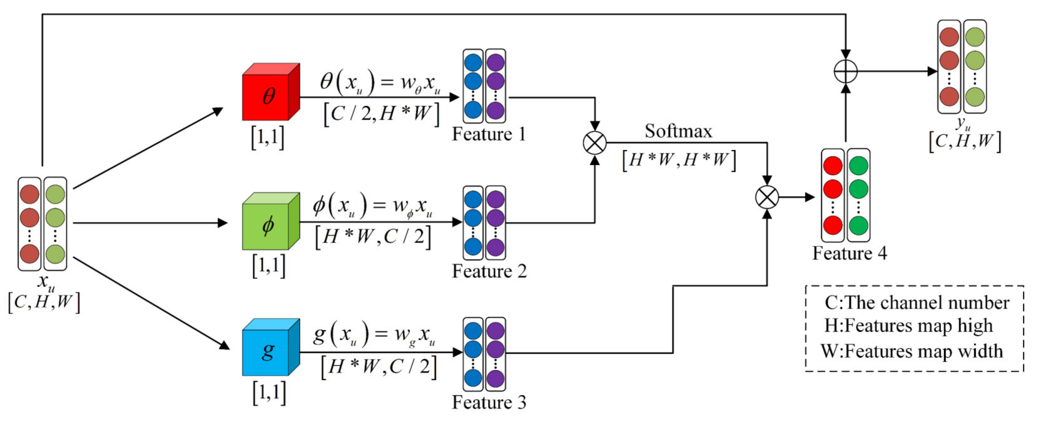
The non-local network is mainly composed of three convolution operators. The main contents are as follows. (1) The long-range correlation information of the feature extracted from samples is calculated. (2) The long-range correlation information is integrated into the features and the output dimension is adjusted to ensure the input and output dimensions are consistent. The flowchart of the non-local network is shown in Figure 1. Firstly, the long-range dependence information of the feature is calculated by the convolution operators and . The equation is expressed as follows:
where and are two convolution operations of . and represent the parameters to be optimized in and , respectively. represents the input features of a non-local network.
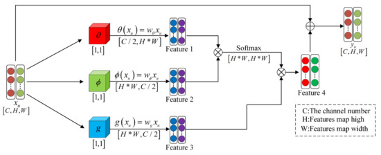
Figure 1.
The flow chart of the non-local module.
Secondly, the long-range correlation information calculated is normalized and it is integrated to the features extracted from the samples. The features with the long-range correlation information are obtained by Equation (4):
where is a convolution operation of . represents the normalization coefficient, and its size depends on the length of the input features. represents the function.
Finally, the idea of residual network is used to ensure that the output dimension is consistent with the input dimension and the input feature information is not lost. Therefore, the non-local network can be inserted after any convolutional layer. The above method can be expressed as the following equation:
where represents the parameter to be optimized.
3. The Proposed Method
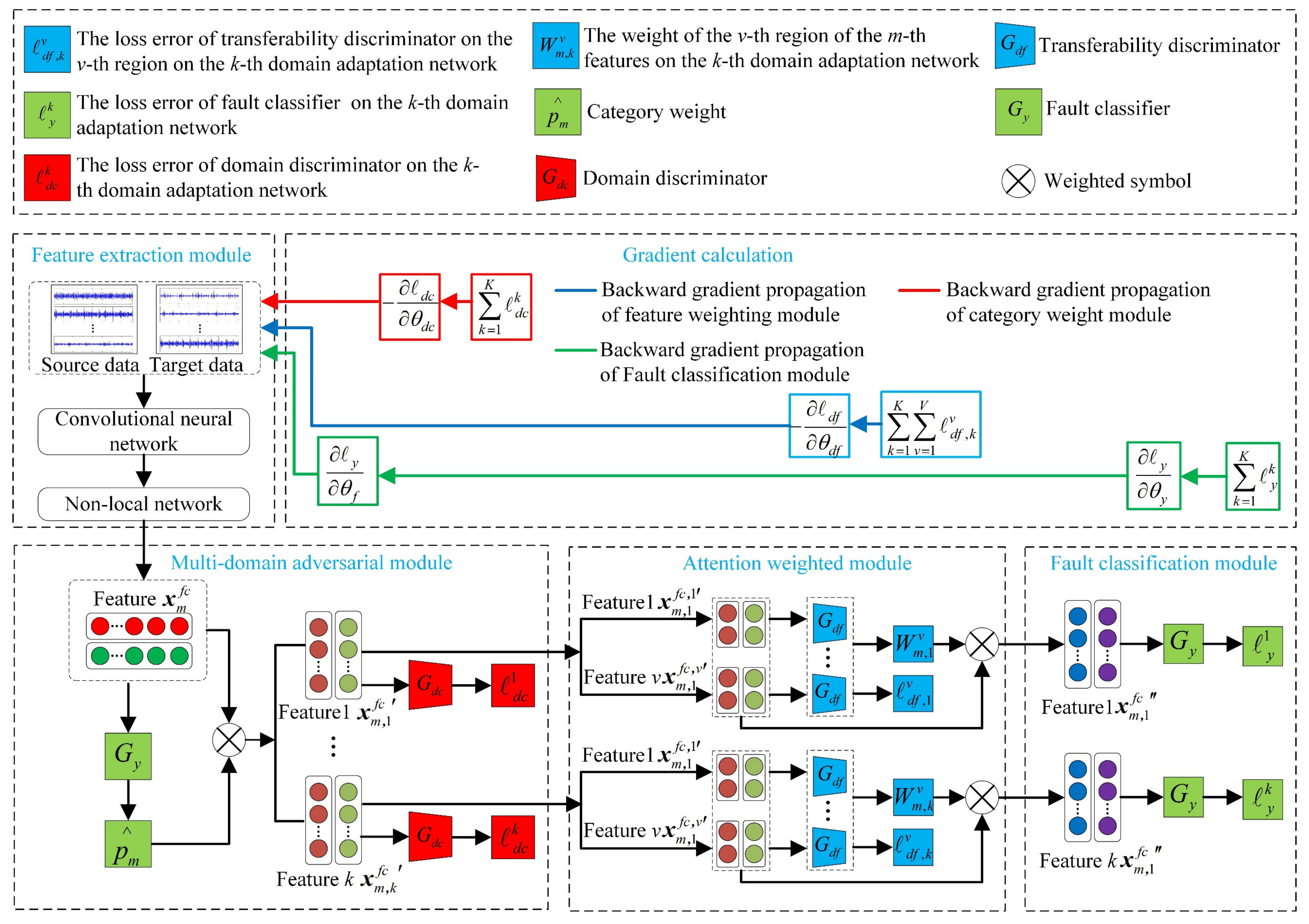
A new method of the multi-domain weighted adversarial transfer network (MWAT) is proposed for the cross-domain intelligent fault diagnosis of bearings. The proposed MWTA mainly includes four parts: feature extraction module, multi-domain adversarial module, attention weighted module and fault classification module. The feature extraction module was used to extract the fault features of the dataset. The multi-domain adversarial module was used to solve the problem of the multi-mode structure of the dataset. The attention weighted module was used to solve the problem that the bearing sample has local non-transferability. Additionally, the fault classification module was optimized to identify the fault states of the bearing dataset. The structure of the MWTA is shown in Figure 2.
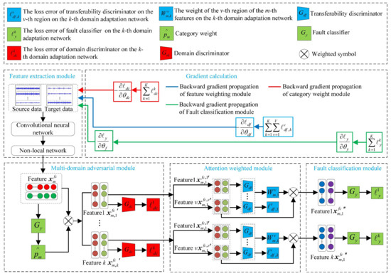
Figure 2.
The structure of the proposed MWTA.
3.1. Feature Extraction Module
The feature extraction module was mainly used to project the dataset of bearings into a high-dimensional feature space, which is composed of a convolutional neural network and a non-local network. Firstly, the features were extracted by a convolutional neural network. Secondly, the long-range correlation information was integrated into the features by a non-local network. Thereby, the connectivity between the different regions of the original data was ensured to enhance the ability of the fault feature extraction.
In this paper, the convolutional neural network was mainly composed of two convolutional layers, one pooling layer, two Rectified Linear Unit (ReLU) layers and one dropout layer. Let the convolutional neural network be expressed as . Therefore, the feature extracted can be expressed as:
where represents the m-th sample in the union of the source and target domains. represents the mapping function of the l-th layer. represents the parameters of the l-th layer to be optimized.
Then, the above features were input into the non-local network. Let the non-local network be expressed as . According to Equations (4) and (5), the features with long-range correlation information can be obtained by Equation (7).
3.2. Multi-Domain Adversarial Module
The source domain and target domain datasets collected contain a variety of different health states, resulting in the datasets present the multi-modal structure. However, the existing transfer fault diagnosis methods directly align the source domain and target domain features without considering the bearing multi-mode structure. When the source domain and target domain data are taken as input for domain adaptation, the source domain features that have a certain information about the health state could match the target domain features that have other information about the health state. The above wrong matching may cause the proposed methods to learn wrong fault information during domain adaptation and affect the accuracy of fault identification. In order to solve the above problem, the multi-domain adversarial module was designed. This module was mainly divided into three steps: (1) The health state type of the features was predicted to capture the bearing multi-mode structure; (2) Multiple domain adaptation networks were established to support the features with different health state types for domain adaptation; and 3) Domain adaptation was performed on each domain adaptation network to reduce the probability of distribution differences of source domain and target domain features.
Firstly, the health state type of the features was predicted to capture the bearings multi-mode structure. Let the fault classifier be , whose specific structure was described in Section 3.4. Furthermore, the feature obtained by Equation (7) was taken as the input feature, and it was assumed that there is a total of k types of health states of bearings. Thus, the output vector of can be expressed as:
where represents the predicted probability of the m-th feature on the k-th health state type. Furthermore, the predicted probability was used as a category weight and assigned to the feature ; thus, the multi-modal structure of the features was captured. Therefore, the weighted features can be expressed as:
Secondly, k domain adaptation networks were established based on the total number k of health state types of bearings. Then, the features , obtained in Equation (9), were input into each domain adaptation network. When the health state information of the source domain and target domain features were consistent, they were assigned to the same domain adaptation network by predicting the probability , thereby solving the problem of the datasets having a multi-mode structure.
Thirdly, based on the features obtained in the second step, domain adaptation was performed in each domain adaptation network by domain adversarial methods; thus, the probability distribution difference of the source domain and target domain features was reduced. Let the domain discriminator on each domain adaptation network be represented as , where the domain discriminator is composed of two fully connected layers, one ReLU layer and one SoftMax layer. The loss error of the domain discriminator on the k-th domain adaptation network is expressed as follows:
where represents the loss function of the domain discriminator on the k-th domain adaptation network; represents the predicted domain label vector of the m-th sample; and represents the real domain label vector of the m-th sample.
The k domains adaptation networks are trained together when the network is training. Therefore, the total loss error of the multi-domain adversarial module can be expressed as:
3.3. Attention Weighted Module
A bearing sample is a vibration signal and it is generally composed of hundreds of continuous sampling points. However, the different regions of a sample may have different transferability due to factors such as working conditions and noise, where some regions that are not suitable for transfer could restrain the decrease in the probability distribution of the source domain and target domain features, resulting in a reduction in the accuracy of fault identification. Therefore, a natural idea is to increase the weight of the sample suitable for transfer regions and reduce the weight of the samples not suitable for transfer regions. Furthermore, the attention weighted module was designed based on above ideas. The attention weighted module included three steps: (1) Features were extracted from the samples to convenient for transferability measurement; (2) The features extracted were divided into v small features of the same length and measuring the transferability of these v small features; and (3) the transferability values obtained in the second step were used as weights that are assigned to the features obtained in the first step.
Firstly, the multi-modal structure of the dataset was solved by the multi-domain adversarial module. Therefore, a reasonable operation is to use the features of the k-th network as the input features of the attention weighted module. It is worth mentioning that an attention weighted module was added to each domain adaptation network to ensure that each feature in the input model was subjected to feature weighting operations.
Secondly, the features of the k-th domain adaptation are equally divided into v small features (the size of v is explained in Section 4.1). The v small features are input into the transferability discriminator to measure the transferability, where the network structure and function of the transferability discriminator and domain discriminator are the same. In this paper, in order to increase the readability in the subsequent loss error calculations, two different symbols were used to name them. The output of the transferability discriminator can be expressed as:
where represents the probability vector of the domain prediction of the v-th small features on the k-th domain adaptation network. represents the v-th small features in the v small features on the k-th domain adaptation network. In information theory, the uncertainty can be measured by an entropy function. Therefore, we can generate the weight of the v-th small feature in the v small features according to the entropy function, where the size of the weight represents the transferability of the v-th small features. This weight is calculated as shown in Equation (13):
where represents the weight of the v-th small features of the m-th feature on the k-th domain adaptation network.
Thirdly, the weights obtained in Equation (13) were assigned to the corresponding regions to obtain new weighted features :
The transferability discriminator was optimized the during training to obtain more accurate weights . The loss error of the transferability discriminator on the k-th domain adaptation network is as follows:
where represents the loss function of the domain discriminator on the v-th small features on the k-th domain adaptation network. represents the predicted domain label vector of the v-th small features on the k-th domain adaptation network. Additionally, represents the real domain label vector of the v-th small features on the k-th domain adaptation network.
The k domains adaptation networks are trained together when the network is training. Therefore, the total loss error of the attention weighted module can be expressed as:
3.4. Fault Classification Module
The fault classification module is mainly composed of fault classifier, where the fault classifier is mainly used to predict the health states of the extracted features. Let the fault classifier be represented as , with the fault classifier being composed of three fully connected layers, one ReLU layer and one SoftMax layer. Therefore, the predicted probability of the fault states of the m-th feature of the k-th network can be obtained according to Equation (17):
Then, the fault classifier is optimized so that its identification accuracy is higher. The loss error of fault classifier is expressed as follows:
where represents the loss function of the fault classifier on the k-th domain adaptation network; represents the predicted probability vector of the m-th feature on the k-th network; and represents the real label vector of the m-th feature on the k-th network.
The k domains adaptation networks are trained together when the network is training. Therefore, the total loss function of the fault diagnosis can be expressed as:
3.5. Objective Loss Function of the Proposed MWTA
According to the objective loss function of the multi-domain adversarial module, attention weighted module and fault classification module, the total objective loss function of MWTA can be expressed as:
where , , and represent, respectively, the parameters of the feature extraction module, multi-domain adversarial module, features weight modules and fault classification module to be optimized. Since the loss function and loss function are both domain discrimination loss errors, let represent the sum of the loss functions and . represents the trade-off parameter between the loss function and loss function of the fault classifier .
Based on Equation (20), the optimization objective of the proposed MWTA was obtained:
The optimization objective was solved by Adam, which is a commonly used optimization algorithm. After the optimization, the training of the MWTA was completed. Finally, the trained MWTA was applied to the cross-domain intelligent fault diagnosis of rolling bearings.
4. Experiments
The proposed method was verified by two intelligent diagnosis cases of bearings, where the diagnosis case 1 was used to verify the transfer fault diagnosis of bearings under different working conditions and the diagnosis case 2 was used to verify the transfer fault diagnosis under of different bearing datasets.
4.1. Diagnosis Case 1: Transfer Fault Diagnosis between Different Working Conditions
In this diagnosis case, the bearing datasets of Case Western Reserve University (CWRU) were selected to verify the transfer diagnosis effect of bearings under different working conditions [36]. Since the CWRU bearing datasets are an open source dataset, the diagnosis results of the proposed method were compared with those of typical methods and published papers, which makes the comparative results more convincing.
4.1.1. Datasets Description
In this dataset, firstly, we selected a bearing monitoring signal under the condition of sampling frequency of 12 kHz and speed of 1797 r/min to construct the bearing datasets. Secondly, the A, B, C and D datasets were sequentially defined according to the dataset of CWRU, which have four different working conditions of 0, 1, 2 and 3 hp. In each working condition, the dataset consisted of ten health states under four fault types and three fault degrees, where four fault types were normal (N), roller fault (RF), inner race fault (IF) and outer race fault (OF), and three fault degrees were 0.18, 0.36 and 0.54 mm. Finally, 1044 sampling points were regarded as one sample, and the dataset under any working condition included 481 normal samples, 450 roller fault samples, 450 inner race fault samples and 450 outer race fault samples. The details of the bearing datasets are shown in Table 1.

Table 1.
Details of the bearing datasets of the diagnosis case 1.
4.1.2. Experimental Tasks
In the engineering practice, the monitoring data of the bearings under no load is easier to obtain than the monitoring data under other load conditions. Therefore, three experimental tasks were set up for the diagnosis case 1, as shown in Table 2. In each of the experimental tasks, the dataset under no-load condition was regarded as the source domain dataset, and the datasets under other load conditions were regarded as the target domain dataset. The experiment task can be expressed in the form of A→B, where the left side of the arrow represents the source domain dataset and the right side of the arrow represents the target domain dataset. In each set of the experimental tasks, all source domain data and 50% target domain data were used as training dataset, and the remaining 50% target domain data were used as the testing dataset.

Table 2.
Transfer diagnosis experiment in the diagnosis case 1.
4.1.3. Experimental Parameters
In the experiment, the proposed method consisted of four parts: feature extraction module, multi-domain adversarial module, attention weighted module and fault classification module. The feature extraction module was composed of a convolutional neural network and a non-local network. The network structure of each part was as follows. The convolutional neural network consisted of seven layers of network, including two convolutional layers, two pooling layers, two ReLU layers and one dropout layer. The non-local network was mainly composed of three convolution operators. The multi-domain adversarial module was mainly composed of k domain discriminator . The attention weighted module was mainly composed of k transferability discriminator . Additionally, the domain discriminator and transferability discriminator had the same network structure, both being composed of two fully connected layers, one ReLU layer and one SoftMax layer. The fault classification module was composed of the fault classifier, where the fault classifier was composed of three fully connected layers, one ReLU layer and one SoftMax layer.
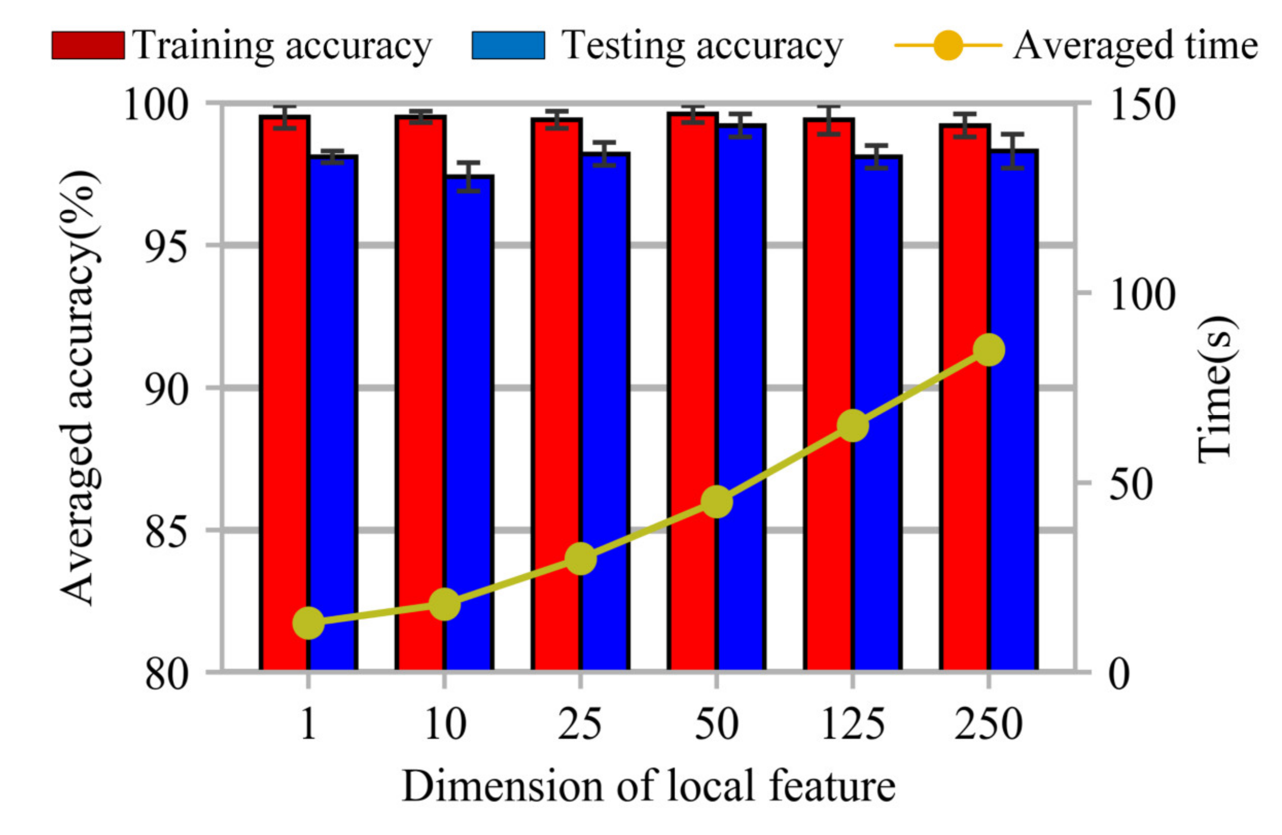
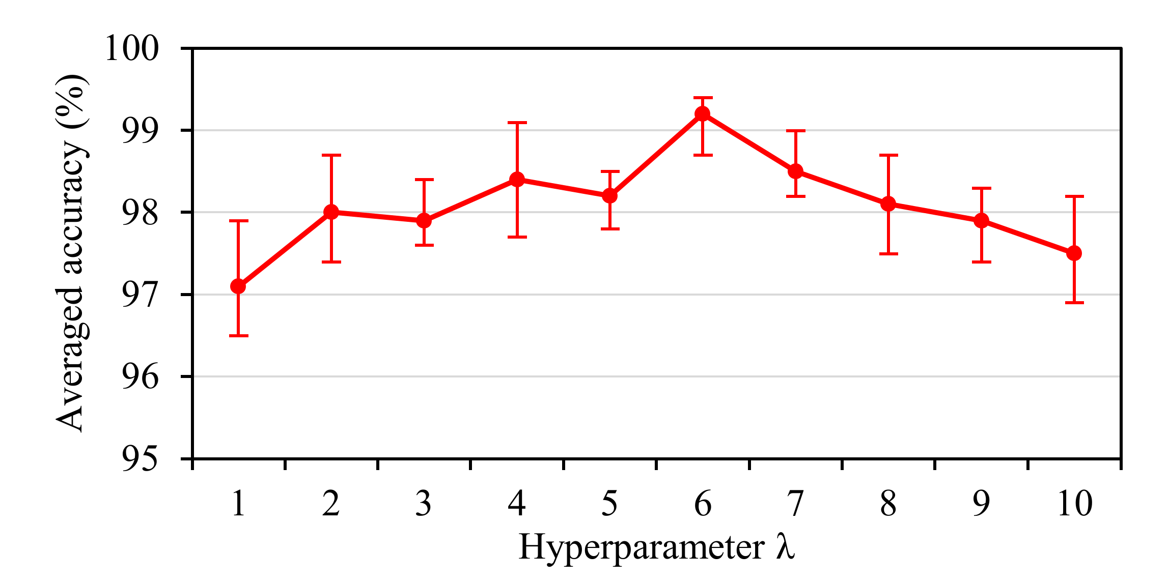
Before the experiments, the hyperparameter V in Section 3.3 and the hyperparameter in Equation (18) needed to be determined, where the size of the hyperparameter v affects the training accuracy and training time, and the hyperparameter is used to balance the loss error of the domain discriminator and fault classification. The experiments were performed on the three groups of experiments in Table 2, and each experiment was repeated 10 times. The experimental results are shown in Figure 3 and Figure 4. It can be seen from Figure 3 that, when the hyperparameter v is 50, it has the highest training accuracy on the testing dataset and the training time is moderate, thus 50 was selected as the value of the hyperparameter v. It can be seen from Figure 4 that, when the hyperparameter takes a value from 1 to 6, the average training accuracy of the proposed method shows an upward trend. Additionally, when the hyperparameter takes a value from 6 to 10, the average training accuracy of the proposed method shows a downward trend. Therefore, 6 was used as the value of the hyperparameter .

Figure 3.
Diagnostic accuracy of the proposed method according to different values of the hyperparameter V.
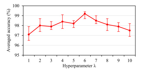
Figure 4.
Diagnosis accuracy of the proposed method according to different values of the hyperparameter .
4.1.4. Diagnosis Results and Comparisons
In order to verify the effectiveness of the proposed method, five typical diagnosis methods were introduced for comparison with the proposed method. The first typical diagnosis method is the wavelet envelope features and support vector machine (WEF-SVM) [37]. In this method, firstly, the bearing signal is decomposed by wavelet envelope analysis. Then, the decomposed signals are used to calculate the wavelet energy ratio. Finally, these energy features are input to the support vector machine for fault classification. The other four typical transfer diagnosis methods are: deep domain confusion maximizing for domain invariance (DDC) [22], domain adaptive neural network (DANN) [34], transferable attention for domain adaptation (TADA) [23] and adversarial discriminative domain adaptation (ADDA) [38]. The experimental tasks are shown in Table 2, and each experimental task was repeatedly trained 10 times. Additionally, the average accuracy of each group of tasks using the different diagnostic methods was counted.
The comparison results between the proposed method and the above five typical methods are shown in Table 3. The final average diagnosis accuracy of WEF-SVM is 78.06%. In the feature extraction of WEF-SVM, the different distribution of the source and target domains is not considered, resulting in a low accuracy. DDC uses the concept of domain confusion to reduce the difference in the feature distribution of the source and target domains, and it obtains an average diagnosis accuracy of 92.70%. DANN uses the idea of adversarial network to confuse the feature extractor, so that the source domain and target domain features extracted by the feature extractor can be on the same feature distribution. Additionally, the final average diagnosis accuracy of DANN is 95.80%. TADA proposed a method to solve the problem of different transferability in different regions of the sample based on the attention mechanism. Additionally, the final average diagnosis accuracy of TADA is 96.53%. ADDA is also based on an idea of adversarial network, hoping to map the source domain network to the target domain, and then obtain an average diagnosis accuracy of 97.40%. For the proposed MWTA, the final average diagnosis accuracy reaches 99.20%. It is seen that the average diagnostic accuracy of the proposed method is higher than other methods, which demonstrates the effectiveness of the proposed method.

Table 3.
The fault identification results of the proposed method and typical methods.
In order to make the comparison results more convincing, we compared the diagnosis results of the proposed method with those of published papers. The comparison results are shown in Table 4. Zhu et al. [39] proposed a bearing fault transfer diagnosis model based on the convolutional neural network (CNN) and maximum mean difference (MMD) methods, and the fault identification accuracy of this model was 94.74%. Xu et al. [40] proposed a method based on transfer component analysis (TCA), and the accuracy of classification could reach 91.40%. Chen et al. [41] proposed the deep neural network (DNN) method, which can achieve a 94.95% accuracy on three-classification tasks. Wang et al. [42] combines the convolutional neural network (CNN) and deep long short-term memory (DLSTM) methods to propose a new transfer model, whose final accuracy of fault identification could reach 96.21%. Li et al. [43] used convolutional neural networks and parameter transfer to achieve a transfer accuracy of 92.25%. Van et al. [44] combined wavelet kernel local fisher discriminant analysis and a support vector machine (SVM) to propose a new classification method, whose accuracy could reach 98.80%. The results show that proposed method has better performance compared with the other fault diagnosis models.

Table 4.
The fault identification results of the proposed method and published papers.
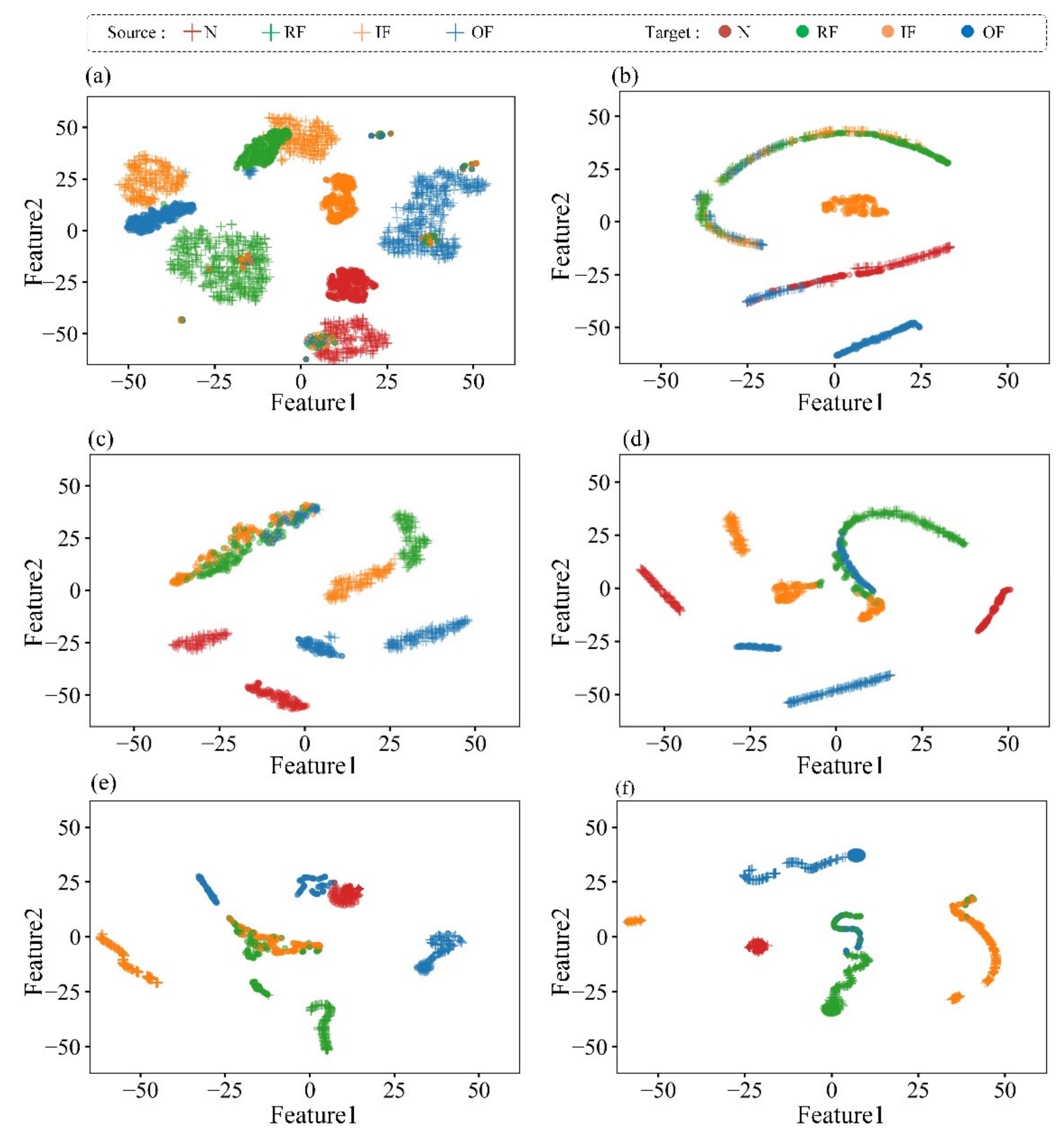
In order to illustrate the alignment of the source domain features and the target domain features in cross-domain fault diagnosis of bearings, we use dT-SNE [45] to visualize these features and visually analyze the diagnosis results of each diagnosis method. The results of the T-SNE feature visualization are shown in Figure 5. The proposed MWTA considers the characteristics of the multi-mode structure between datasets and the transferability between different regions of the sample. In the features space, the features of the source and target domains of the same fault states merge with each other, and their distribution tends to be similar. Meanwhile, the features of different health states are separated from each other to ensure the accuracy of fault identification. Therefore, compared with the other five methods, the proposed method can obtain a higher fault identification accuracy.
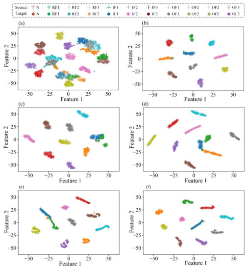
Figure 5.
T-SNE feature visualization results of on six methods: (a) WEF-SVM, (b) ADDA, (c) DDC, (d) DANN, (e) TADA and (f) the proposed MWTA.
4.2. Diagnosis Case 2: Transfer Fault Diagnosis between Different Bearings
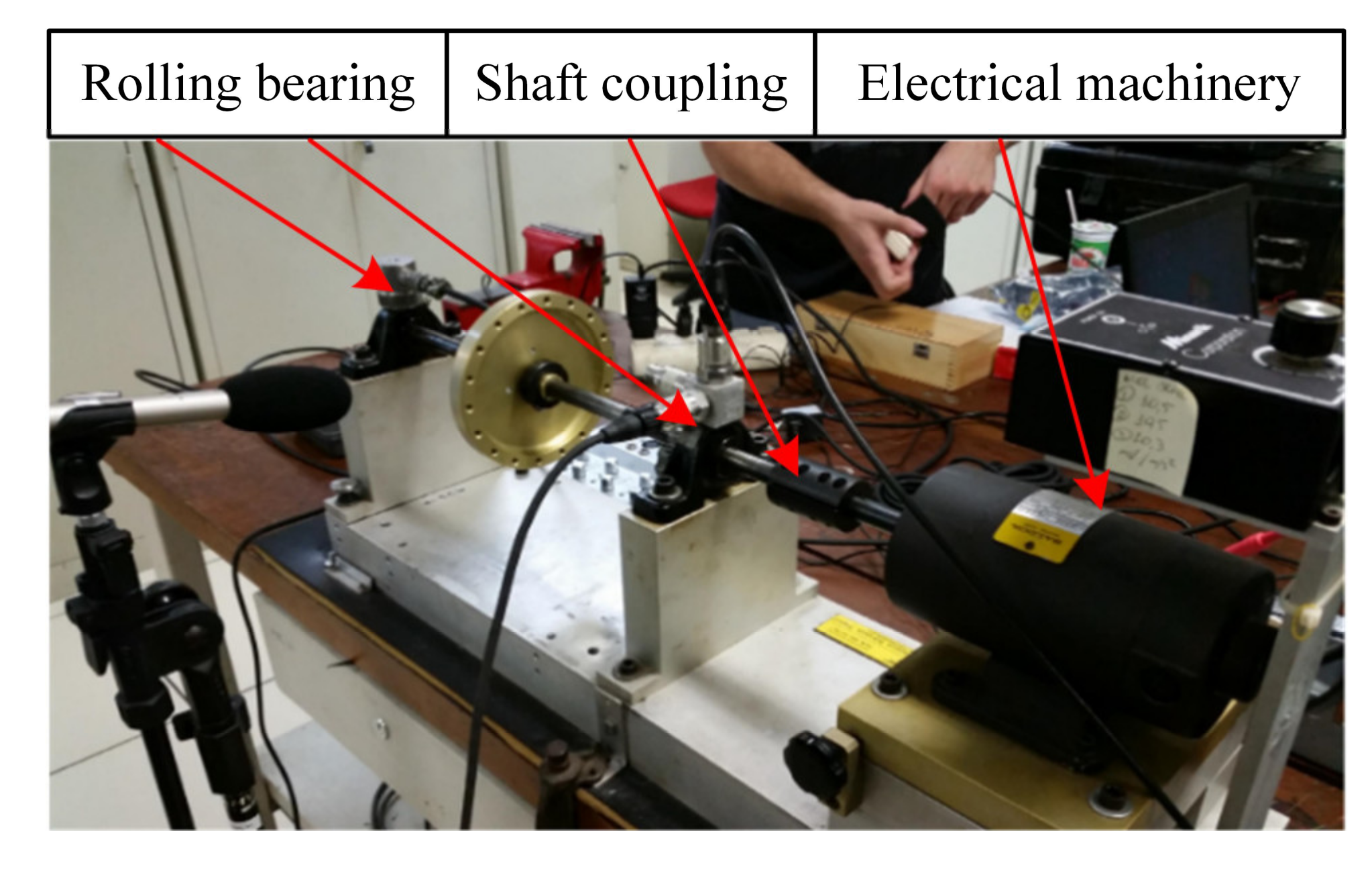
The experimental data of this diagnosis case were obtained from Case Western Reserve University bearing datasets, SpectraQuest’s mechanical failure simulator [46] and gearbox bearing failure test bench. The SpectraQuest’s mechanical failure simulator is shown in Figure 6 and the gearbox bearing failure test bench is shown in Figure 7.

Figure 6.
SpectraQuest’s mechanical failure simulator.
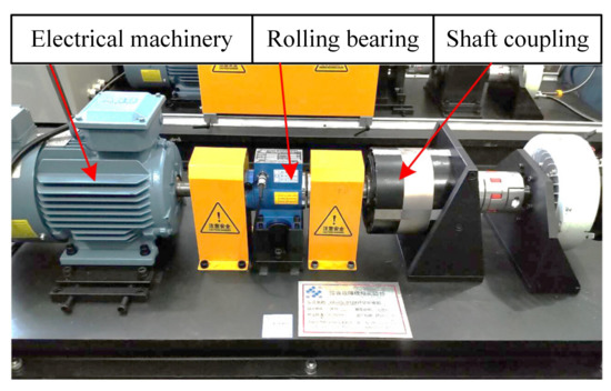
Figure 7.
Gearbox bearing failure test bench.
4.2.1. Data Collection
In the experiment, the three different bearing datasets, obtained from Case Western Reserve University bearing datasets, SpectraQuest’s mechanical failure simulator and Gearbox bearing failure test bench, were defined as dataset E, dataset F and dataset G, respectively. The three different bearing datasets all contained four different health states: normal (N), roller fault (RF), inner race fault (IF) and outer race fault (OF). The sampling frequency of dataset E was 12 kHZ, the number of samples was 1710, and the rotation speed and load conditions of the bearing equipment were 1772 r/min and 1 Hp, respectively. The sampling frequency of dataset F was 5 kHZ, the number of samples was 1528, and the rotation speed and load conditions of the bearing equipment were 1528 r/min and 6 g, respectively. The sampling frequency of dataset G was 5 kHZ, the number of samples was 2400, and the rotation speed and load conditions of the bearing equipment were 600 r/min and 3 N*mm. The comparison results of the three datasets are shown in Table 5.

Table 5.
Details of the bearing datasets of the diagnosis case 2.
4.2.2. Experimental Task
For three different bearing datasets, six groups of experimental tasks were set, as shown in Table 6. The experiment task were expressed in the form of E→F, where the left side of the arrow represents the source domain dataset and the right side of the arrow represents the target domain dataset. Additionally, in each set of the experimental tasks, all source domain data and 50% target domain data were used as the training dataset, and the remaining 50% target domain data were used as the testing dataset.

Table 6.
Transfer diagnosis experiment in the diagnosis case 2.
4.2.3. Diagnosis Results and Comparisons
The proposed method was compared with the five typical transfer intelligent diagnosis methods introduced in Section 4.1.3. The comparison results of the experiments are shown in Table 7. The results show that the average diagnosis result of the proposed MWTA can reach 85.60% and the diagnosis accuracy of the other five methods varies from 40.54% to 77.50%. Through comparative analysis, the diagnosis result of the proposed method is better than those of the other methods, which proves the effectiveness of the proposed method. Furthermore, the extracted features of each method were visualized by T-SNE, and the feature visualization results are shown in Figure 8. It can be seen that, compared with the other methods, the proposed method can effectively align the feature distributions of the source and target domains, and the features of different health states were distinguished well. Therefore, the proposed method can improve the identification accuracy of cross-domain fault diagnosis under different bearings by considering the multi-mode data structure and the local non-transferable characteristics of the samples.

Table 7.
The fault identification results of the proposed method and typical method.
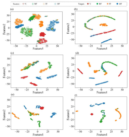
Figure 8.
T-SNE visualization results of on the six methods, where (a) WEF-SVM, (b) ADDA, (c) DDC, (d) DANN, (e) TADA and (f) the proposed MWTA.
5. Conclusions
In order to consider the characteristics of the bearing multi-modal structure and the transferability of the sample local regions, a multi-domain weighted transfer adversarial network was proposed for the cross-domain intelligent fault diagnosis of bearings. The proposed method considers the multi-mode structure of the bearing dataset by designing a multi-domain adversarial module and solves the problem that different regions of the bearing signals have different transferability by designing an attention weighted module. Through two fault diagnosis cases, it was illustrated that the proposed method can effectively reduce the difference of the probability distribution between the source domain and target domain datasets, thereby improving the cross-domain fault diagnosis accuracy. In addition, it can be seen from Table 3 and Table 7 that, for the first case, the accuracy of cross-domain fault diagnosis increased by 7.10% on average, and for the second case, the accuracy of cross-domain fault diagnosis increased by 21.17%, indicating that this method can significantly improve the accuracy of cross-domain fault diagnosis.
Author Contributions
Conceptualization, Y.W. and S.L.; methodology, Y.W. and S.L.; software, Y.W. and S.L.; validation, F.J. and S.L.; formal analysis, F.J.; investigation, J.S.; resources, F.J. and J.S.; data curation, Y.W. and S.L.; writing—original draft preparation, Y.W. and S.L.; writing—review and editing, Y.W. and S.L.; visualization, Y.W. and S.L.; supervision, J.S.; project administration, F.J. All authors have read and agreed to the published version of the manuscript.
Funding
This research was supported by National Natural Science Foundation of China (No. 52105085), Shaanxi Provincial Natural Science Basic Research Program (No. 2020JQ-365) and China Postdoctoral Science Foundation (No. 2020M683393).
Institutional Review Board Statement
Not applicable.
Informed Consent Statement
Not applicable.
Data Availability Statement
The available data that support the findings of this study were obtained from the data source of Case Western Reserve University’s Electrical Engineering Laboratory and SpectraQuest’s mechanical failure simulator.
Conflicts of Interest
The authors declare no conflict of interest.
References
- Li, W.; Huang, R.; Li, J.; Liao, Y. A perspective survey on deep transfer learning for fault diagnosis in industrial scenarios. Theories, applications and challenges. Mech. Syst. Signal Process. 2022, 167, 108487. [Google Scholar] [CrossRef]
- Zhao, Z.; Zhang, Q.; Yu, X. Applications of Unsupervised Deep Transfer Learning to Intelligent Fault Diagnosis. A Survey and Comparative Study. IEEE Trans. Instrum. Meas. 2021, 70, 3525828. [Google Scholar] [CrossRef]
- Wu, J.-D.; Luo, W.-J.; Yao, K.-C. Acoustic Signal Classification Using Symmetrized Dot Pattern and Convolutional Neural Network. Machines 2022, 10, 90. [Google Scholar] [CrossRef]
- Kudelina, K.; Baraškova, T.; Shirokova, V.; Vaimann, T. Fault Detecting Accuracy of Mechanical Damages in Rolling Bearings. Machines 2022, 10, 86. [Google Scholar] [CrossRef]
- Irfan, M. Modeling of Fault Frequencies for Distributed Damages in Bearing Raceways. J. Nondestruct. Eval. 2019, 38, 98. [Google Scholar] [CrossRef]
- Wen, L.; Li, X.; Gao, L.; Zhang, Y. A New Convolutional Neural Network-Based Data-Driven Fault Diagnosis Method. IEEE Trans. Ind. Electron. 2018, 65, 5990–5998. [Google Scholar] [CrossRef]
- Shao, H.; Jiang, H.; Zhang, H.; Liang, T. Electric Locomotive Bearing Fault Diagnosis Using a Novel Convolutional Deep Belief Network. IEEE Trans. Ind. Electron. 2017, 65, 2727–2736. [Google Scholar] [CrossRef]
- Zhang, F.; Yan, J.; Fu, P.; Gao, R. Ensemble sparse supervised model for bearing fault diagnosis in smart manufacturing. Robot. Comput.-Integr. Manuf. 2020, 65, 101920. [Google Scholar] [CrossRef]
- Li, Y.; Yang, Y.; Wang, X.; Liu, B.; Liang, X. Early fault diagnosis of rolling bearings based on hierarchical symbol dynamic entropy and binary tree support vector machine. J. Sound Vib. 2018, 428, 72–86. [Google Scholar] [CrossRef]
- Liu, D.; Li, Q.; Hu, W.; Pan, W. Fatigue life prediction of the axle box bearings for high-speed trains. Dyna 2017, 92, 538–544. [Google Scholar] [CrossRef] [Green Version]
- Liu, Z.; Zuo, M.; Qin, Y. Remaining useful life prediction of rolling element bearings based on health state assessment. Proc. Inst. Mech. Eng. Part C J. Mech. Eng. Sci. 2016, 230, 314–330. [Google Scholar] [CrossRef] [Green Version]
- Ma, B.; Zhai, B.; Peng, Q.; Wang, Y. Useful life prediction of rolling element bearings based on a particle filtering model and the state space model at different degradation stages. J. Beijing Univ. Chem. Technol. Nat. Sci. Ed. 2017, 44, 81–86. [Google Scholar]
- Al-Moslmi, T.; Omar, N.; Abdulah, S.; Albared, M. Approaches to Cross-Domain Sentiment Analysis: A Systematic Literature Review. IEEE Access 2017, 5, 16173–16192. [Google Scholar] [CrossRef]
- Du, Z.; Yang, B.; Lei, Y.; Li, X.; Li, N. A Hybrid Transfer Learning Method for Fault Diagnosis of Machinery under Variable Operating Conditions. In Proceedings of the 2019 Prognostics and System Health Management Conference (PHM-Qingdao), Qingdao, China, 25–27 October 2019; p. 5. [Google Scholar]
- Yang, B.; Lei, Y.; Jia, F.; Li, N.; Du, Z. A Polynomial Kernel Induced Distance Metric to Improve Deep Transfer Learning for Fault Diagnosis of Machines. IEEE Trans. Ind. Electron. 2020, 67, 9747–9757. [Google Scholar] [CrossRef]
- Guo, L.; Lei, Y.; Xing, S.; Yan, T.; Li, N. Deep Convolutional Transfer Learning Network: A New Method for Intelligent Fault Diagnosis of Machines with Unlabeled Data. IEEE Trans. Ind. Electron. 2019, 66, 7316–7325. [Google Scholar] [CrossRef]
- Zou, Y.; Liu, Y.; Deng, J.; Jiang, Y.; Zhang, W. A novel transfer learning method for bearing fault diagnosis under different working conditions. Measurement 2021, 171, 108767. [Google Scholar] [CrossRef]
- Pei, Z.; Cao, Z.; Long, M.; Wang, J. Multi-Adversarial Domain Adaptation. arXiv 2018, arXiv:1809.02176. [Google Scholar]
- Chen, Z.; Guo, L.; Gao, H.; Yu, Y.; Wu, W.; You, Z.; Dong, X. A fault pulse extraction and feature enhancement method for bearing fault diagnosis. Measurement 2021, 182, 109718. [Google Scholar] [CrossRef]
- Han, B.; Zhang, X.; Wang, J.; An, Z.; Zhang, G. Hybrid distance-guided adversarial network for intelligent fault diagnosis under different working conditions. Measurement 2021, 176, 109197. [Google Scholar] [CrossRef]
- Tan, Y.; Guo, L.; Gao, H.; Lin, Z.; Liu, Y. MiDAN: A framework for cross-domain intelligent fault diagnosis with imbalanced datasets. Measurement 2021, 183, 109834. [Google Scholar] [CrossRef]
- Tzeng, E.; Hoffman, J.; Zhang, N.; Saenko, K.; Darrell, T. Deep Domain Confusion: Maximizing for Domain Invariance. arXiv 2014, arXiv:1412.3474. [Google Scholar]
- Wang, X.; Li, L.; Ye, W.; Long, M.; Wang, J. Transferable Attention for Domain Adaptation. In Proceedings of the Thirty-Third AAAI Conference on Artificial Intelligence and Thirty-First Innovative Applications of Artificial Intelligence Conference and Ninth AAAI Symposium on Educational Advances in Artificial Intelligence, Honolulu, HI, USA, 27 January–1 February 2019; pp. 5345–5352. [Google Scholar]
- Wang, R.; Zhang, S.; Chen, Z.; Li, W. Enhanced generative adversarial network for extremely imbalanced fault diagnosis of rotating machine. Measurement 2021, 180, 109467. [Google Scholar] [CrossRef]
- Xu, K.; Li, S.; Jiang, X.; An, Z. A renewable fusion fault diagnosis network for the variable speed conditions under unbalanced samples. Neurocomputing 2020, 379, 12–29. [Google Scholar] [CrossRef]
- Zhao, X.; Jia, M.; Lin, M. Deep Laplacian Auto-encoder and its application into imbalanced fault diagnosis of rotating machinery. Measurement 2020, 152, 107320. [Google Scholar] [CrossRef]
- Pan, S.J.; Yang, Q. A Survey on Transfer Learning. IEEE Trans. Knowl. Data Eng. 2010, 22, 1345–1359. [Google Scholar] [CrossRef]
- Long, J.; Zhang, S.; Li, C. Evolving Deep Echo State Networks for Intelligent Fault Diagnosis. IEEE Trans. Ind. Inform. 2020, 16, 4928–4937. [Google Scholar] [CrossRef]
- Chen, C.; Shen, F.; Xu, J.; Yan, R. Domain Adaptation Based Transfer Learning for Gear Fault Diagnosis under Varying Working Conditions. IEEE Trans. Instrum. Meas. 2020, 70, 1–10. [Google Scholar] [CrossRef]
- Li, Q.; Shen, C.; Chen, L.; Zhu, Z. Knowledge mapping-based adversarial domain adaptation: A novel fault diagnosis method with high generalizability under variable working conditions. Mech. Syst. Signal Process. 2021, 147, 107095. [Google Scholar] [CrossRef]
- Zhang, L. Transfer Adaptation Learning: A Decade Survey. arXiv 2019, arXiv:1903.04687. [Google Scholar]
- Tan, C.; Sun, F.; Kong, T.; Zhang, W.; Yang, C.; Liu, C. A Survey on Deep Transfer Learning. In Proceedings of the 27th International Conference on Artifical Neural Network (ICANN), Rhodes, Greece, 4–7 October 2018; Volume 11141, pp. 270–279. [Google Scholar]
- Wen, L.; Li, X.; Gao, L. A transfer convolutional neural network for fault diagnosis based on ResNet-50. Neural Comput. Appl. 2020, 32, 6111–6124. [Google Scholar] [CrossRef]
- Ghifary, M.; Kleijn, W.B.; Zhang, M. Domain Adaptive Neural Networks for Object Recognition. In Proceedings of the 13th Pacific Rim International Conference on Artificial Intelligence (PRICAI), Gold Coast, Australia, 1–5 December 2014; Volume 8862, pp. 898–904. [Google Scholar]
- Wang, X.; Girshick, R.; Gupta, A.; He, K. Non-local Neural Networks. arXiv 2017, arXiv:1711.07971. [Google Scholar]
- Li, X.; Zhang, W.; Ding, Q.; Li, X. Diagnosing Rotating Machines with Weakly Supervised Data Using Deep Transfer Learning. IEEE Trans. Ind. Inform. 2020, 16, 1688–1697. [Google Scholar] [CrossRef]
- Nikravesh, S.M.Y.; Rezaie, H.; Kilpatrik, M.; Taheri, H. Intelligent Fault Diagnosis of Bearings Based on Energy Levels in Frequency Bands Using Wavelet and Support Vector Machines (SVM). J. Manuf. Mater. Process. 2019, 3, 11. [Google Scholar]
- Tzeng, E.; Hoffman, J.; Saenko, K.; Darrell, D. Adversarial Discriminative Domain Adaptation. In Proceedings of the 2017 IEEE Conference on Computer Vision and Pattern Recognition (CVPR), Honolulu, HI, USA, 21–26 July 2017. [Google Scholar] [CrossRef]
- Zhu, J.; Chen, N.; Shen, C. A New Deep Transfer Learning Method for Bearing Fault Diagnosis Under Different Working Conditions. IEEE Sens. J. 2020, 20, 8349–8402. [Google Scholar] [CrossRef]
- Xu, W.; Wan, Y.; Zuo, T.; Sha, X. Transfer Learning Based Data Feature Transfer for Fault Diagnosis. IEEE Access 2020, 8, 76120–76129. [Google Scholar] [CrossRef]
- Chen, D.; Yang, S.; Zhou, F. Incipient Fault Diagnosis Based on DNN with Transfer Learning. In Proceedings of the 7th International Conference on Control Automation and Information Sciences (ICCAIS), Hangzhou, China, 24–27 October 2018; pp. 303–308. [Google Scholar]
- Wang, Z.; Liu, Q.; Chen, H.; Chu, X. A deformable CNN-DLSTM based transfer learning method for fault diagnosis of rolling bearing under multiple working conditions. Int. J. Prod. Res. 2020, 59, 4811–4825. [Google Scholar] [CrossRef]
- Li, F.; Chen, J.; Pan, J.; Pan, T. Cross-domain learning in rotating machinery fault diagnosis under various operating conditions based on parameter transfer. Meas. Sci. Technol. 2020, 31, 8. [Google Scholar] [CrossRef]
- Van, M.; Kang, H.J. Bearing Defect Classification Based on Individual Wavelet Local Fisher Discriminant Analysis with Particle Swarm Optimization. IEEE Trans. Ind. Inform. 2015, 12, 124–135. [Google Scholar] [CrossRef]
- Kang, B.; García, D.G.; Lijffijt, J. Conditional t-SNE: More informative t-SNE embeddings. In Proceedings of the 2021 IEEE 8th International Conference on Data Science and Advanced Analytics (DSAA), Porto, Portugal, 6–9 October 2021; pp. 1–2. [Google Scholar]
- Marins, M.A.; Ribeiro, F.M.L.; Netto, S.L.; Silva, E. Improved similarity-based modeling for the classification of rotating-machine failures. J. Frankl. Inst. 2018, 355, 1913–1930. [Google Scholar] [CrossRef]
Publisher’s Note: MDPI stays neutral with regard to jurisdictional claims in published maps and institutional affiliations. |
© 2022 by the authors. Licensee MDPI, Basel, Switzerland. This article is an open access article distributed under the terms and conditions of the Creative Commons Attribution (CC BY) license (https://creativecommons.org/licenses/by/4.0/).

