Abstract
The quality, wear and safety of metal structures can be controlled effectively, provided that surface defects, which occur on metal structures, are detected at the right time. Over the past 10 years, researchers have proposed a number of neural network architectures that have shown high efficiency in various areas, including image classification, segmentation and recognition. However, choosing the best architecture for this particular task is often problematic. In order to compare various techniques for detecting defects such as “scratch abrasion”, we created and investigated U-Net-like architectures with encoders such as ResNet, SEResNet, SEResNeXt, DenseNet, InceptionV3, Inception-ResNetV2, MobileNet and EfficientNet. The relationship between training validation metrics and final segmentation test metrics was investigated. The correlation between the loss function, the , , , and validation metrics and test metrics was calculated. Recognition accuracy was analyzed as affected by the optimizer during neural network training. In the context of this problem, neural networks trained using the stochastic gradient descent optimizer with Nesterov momentum were found to have the best generalizing properties. To select the best model during its training on the basis of the validation metrics, the main test metrics of recognition quality (Dice similarity coefficient) were analyzed depending on the validation metrics. The ResNet and DenseNet models were found to achieve the best generalizing properties for our task. The highest recognition accuracy was attained using the U-Net model with a ResNet152 backbone. The results obtained on the test dataset were and .
1. Introduction
The quality control of rolled metal remains a complex technical and technological problem [1,2,3]. A rolled surface free from defects ensures a high product quality and efficient further metal processing. Detecting defects on the metal surface is an important step in the quality management of metallurgical production [4]. To date, defects have been detected using optical-digital systems that allow obtaining and processing strip surface images on a computer [5,6,7,8,9,10]. There are a significant number of algorithms for detecting defects, which are being constantly improved [11,12,13].
A significant number of research works dedicated to this problem have assisted in creating a system of methods and technical instruments to control hot and cold rolled metal surfaces. The general principles and approaches to the solution of defectoscopic and defectometric problems have been developed and physically substantiated, and the peculiarities of certain metallurgical defects have been described. However, individual features of the technological process account for the occurrence of defects by causing certain morphological features thereof, which require further description and generalization [14,15]. Therefore, investigations aimed at improving the methods for recognizing surface defects of rolled metal, in particular those taking into account the influence of technological factors, are relevant.
Over the past 15 years, automated detection of defects based on machine vision has attracted the attention of many researchers, resulting in solutions for a number of theoretical and applied problems. Defect segmentation, which allows creating a binary map of a defective surface, is important in the process of automatic inspection of a surface condition. Segmentation is performed using various methods. Statistical methods (Otsu’s method, gray-level co-occurrence matrix, etc.) are based on calculating the spatial distribution of the image pixel intensity. Methods based on filters (discrete Fourier or Gabor transformation, wavelet transformation, etc.) highlight features of the objects of interest using a filter bank. In 2015, a trend in the recognition of surface defects was started by the machine vision methods, which eliminate both the numerous shortcomings of manual detection, and the excessive complexity of statistical and filter-based methods. Such systems have already been adopted by many industries, including for monitoring the condition of metal surfaces and semiconductor products, fabric inspection, detecting damage to the road surface and civil structures, railway track inspection and food control.
Defects of metal surfaces can vary in size, shape and texture and often bear substantial similarities to possible surface artifacts that are not defects in themselves. Therefore, developing a universal and effective segmentation method for quantifying such defects takes a lot of effort. At the same time, artificial neural networks make it possible to create a complete set of features inherent in defects during training and detect them effectively.
In [11], a multidisciplinary model was proposed to detect surface defects of different classes and the degree of their severity on steel surfaces. The model contains two branches, one of which serves to detect the defect class, and the other to form a severity heat map of the defect. Each branch performs segmentation of the input image by solving the related problems of defect localization and construction of the damage severity map. The resulting model allows recognizing up to 16 classes of defects, as well as estimating the defect severity on a three-point scale. The best model attained when recognizing defects, and when determining the defect’s severity.
An architecture based on a deep convolutional neural network for defect detection on metal surfaces was proposed in [12]. The cascade autoencoder considered allows detecting a pixel mask that contains only damage. A compact convolutional neural network (CNN) is used to quickly calculate the defect class. The method-specific IoU metric calculated on an industrial set of images was 0.896. The results obtained indicated that the method meets the reliability and accuracy requirements placed on the detection of metal defects.
The authors of [13] investigated the defects of titanium-coated metal surfaces and proposed a model based on the deep convolutional U-Net model. The proposed method includes pre-processing of the image and post-processing of the result using morphological operators to eliminate unacceptable artifacts. The proposed technique allows recognizing damage with . In [14], a method for the automated recognition of defects in steel production was developed and investigated. To this end, a series of machine learning algorithms for real-time semantic segmentation were used, as well as a CNN with a U-Net-based encoder–decoder architecture and a feature pyramid network. Using the proposed approach, the researchers achieved 0.915 and values.
In [15], an adaptive depth and receptive field selection network for the semantic segmentation of defects in castings was presented. The ResNet18 CNN with an adaptive depth selection mechanism was used for this purpose, which was designed to extract and adaptively combine different features in order to detect defects. The proposed method attained . The authors of [16] developed and investigated a semantic segmentation method to detect defects on the safety valve of an accumulator battery during laser welding. The proposed model consists of an improved Res2Net, which acts as a sub-module for extracting features, an attention mechanism, a localization unit and a module for smoothing boundaries. The architecture can segment defects of different sizes and shapes in real time and obtain more accurate segmentation results at the same time. was attained. In [17], a CNN-based method was developed for the automatic detection and segmentation of defects on railway tracks. The developed technique allows conducting segmentation with .
Thus, there are a number of approaches to defect recognition that use different neural network architectures, and different training and hyperparameter selection techniques. Typically, the proposed neural network model is trained on a closed dataset, which makes it difficult to compare the results of its work with those of other similar models. This is because creating and testing many different models is fairly laborious and time-consuming. Therefore, the choice of architecture is often poorly justified: researchers usually propose and study a model, demonstrating its practical value. Whenever a model is trained to recognize several classes of damage, its cognitive ability to form feature maps for each individual class is somewhat lowered. Therefore, the maximum possible model accuracy for detecting a particular defect class is often unknown, which may be relevant in cases where the defect detection quality is more important than the list of defects available for the model.
The objective of our research was to build a number of semantic segmentation models with different U-Net-like architectures, investigate the impact of the optimizer model on the final accuracy and different validation metrics, compare the results on one dataset and obtain the best model for one class. The task of choosing the best model also requires the formulation of selection criteria for models obtained during training. For this purpose, it is necessary to investigate the dependence of the validation and test quality metrics of the models. To achieve the maximum accuracy in detecting defects, the model focuses on one of the most common defect types, that is, “scratch abrasion”.
2. Basic Neural Network Architecture for U-Net Semantic Segmentation
The U-Net neural network was developed in 2015 for the processing of medical images [18]. Its architecture results from the development and improvement of conventional convolutional neural networks. Defectometry problems are not restricted solely to classifying images into those that contain and do not contain defects. It is also important to locate damage accurately. In addition to improving product quality control, this allows calculating the quantitative characteristics of damage (area, direction, etc.). This also makes it possible to better understand the nature of damage and develop steps to eliminate it. To achieve this, the U-Net neural network provides for the semantic segmentation of images, where each image pixel is classified as belonging to one of the damage classes, or to the undamaged area. In this case, the input and output images have the same size.
The general architecture of the basic U-Net neural network is shown in Figure 1 [18]. It is symmetrical and contains two main parts: the compression part, i.e., the encoder (on the left), and the expansion part, i.e., the decoder (on the right). The compression part is a typical architecture of a convolutional neural network, which contains repetitive convolutions with a 3 × 3 kernel, followed by the ReLU (rectified linear unit) and max pooling operations. With each downsampling, the number of feature maps doubles.
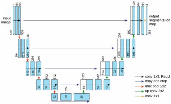
Figure 1.
General architecture of the U-Net neural network. Blue rectangles indicate multichannel feature maps. The number of channels is given above. Copied feature maps are marked with white rectangles. The feature map size is indicated near the lower left edge. Arrows indicate the operation direction.
As the image expands, it gradually enlarges to its original size. Each step of the expansion part increases the dimensions of the feature maps, performs a deconvolution, which halves the number of feature maps, and combines them with the corresponding feature map from the compression part. Combining the image with the convolution result of the previous layer provides for a greater accuracy. At the end of each upsampling, a convolution with a 3 × 3 kernel and ReLU activation function is applied. As a result of the expanded upsampling, new pixels are inserted between the existing ones, until the image attains the required size. The final layer uses a 1 × 1 convolution, which projects each vector with features to the desired number of classes.
3. Investigation of U-Net-like Neural Networks for Segmentation of Images with Defects
3.1. Models for Semantic Segmentation Based on U-Net with Different Backbones
U-Net-based semantic segmentation models have proven effective in various areas where image segmentation is used [19,20,21,22,23]. In this case, convolutional state-of-the-art models that have demonstrated high accuracy can be used as encoders. In our previous work [24,25,26], we investigated deep convolutional residual neural networks as applied to recognizing damage of various types in industrial photos of rolled metal. In particular, we studied neuron activation maps used by the neural network when deciding on the presence of damage [26]. To this end, Gradient-weighted Class Activation Mapping (Grad-CAM) was used. Due to Grad-CAM, we can visually validate our network, verifying that it is indeed looking at the correct patterns in the image and activating around those patterns.
The resulting feature maps were found to be good at reflecting the damage position, size and shape. Those areas of the convolutional layers that correspond to the image portions with defects were shown to be activated during classification. Thus, when detecting defects, the model focuses on their features. Therefore, for the semantic segmentation of images with surface defects, it was decided to use the U-Net architecture with backbones represented by modern models that have proven their effectiveness in image processing, instead of the original version of the U-Net model. The following state-of-the-art architectures have been studied as the basis for the U-Net encoder: ResNet [27], SEResNet, SEResNeXt [28], DenseNet [29], InceptionV3 [30,31], Inception-ResNetV2 [32], MobileNet [33] and EfficientNet [34]. These networks have many modifications depending on the number of layers, including ResNet18 and EfficientNet-b0. These modifications have proven themselves to solve various applications, thus making it possible to find the right balance between the recognition accuracy and learning rate.
Each of these architectures has proven itself in various areas related to image processing. Therefore, we can assume that their use as a backbone for the semantic segmentation model will also be successful. These architectures differ not only in internal structure, but also in complexity. Thus, simpler models may be less accurate, but more acceptable for rapid surface analysis. At the same time, more complex models may run slower but accumulate more features of defects and, as a result, better recognize them.
3.1.1. ResNet
The ResNet architecture was proposed in 2015 by Microsoft researchers and allowed for the construction of deep convolutional networks with high learning rates [27]. Such neural networks have shown excellent results in various areas related to image processing. The ResNet model consists of series-connected residual blocks. Each block contains three layers, which perform 1 × 1 and 3 × 3 convolutions. However, the main feature of ResNet models is shortcut connections. They pass one or more layers and connect the input of one layer (layer) with the output of another. Using shortcut connections significantly reduces the problem of the vanishing gradient in deeper layers of the network and significantly increases the model depth. This advantage makes it relatively easy to optimize ResNet networks, because the learning error does not increase so sharply with an increase in the model depth. Due to its structural features, even the 152-layer ResNet model is less complex than the 16-layer VGG-16 networks (11.3 vs. FLOP 15.3 billion). ResNet was the winner of the ILSVRC 2015 challenge in image classification, detection and localization [35], as well as the winner of the MS COCO 2015 challenge in image detection and segmentation [36].
3.1.2. SEResNet and SEResNeXt
These neural networks are modifications of the basic ResNet architecture. Instead of an equal representation of all feature channels in a layer, these architectures implement a weighted representation [28]. Feature maps are generated per channel (e.g., RGB) and then summed together to form one channel or the final output of the convolution operation. Consequently, the convolution kernel has different weights for different channels. The weights of each channel are learned in a squeeze-and-excitation (SE) block. A squeeze-and-excitation block is applied at the end of each non-identity branch of the residual block. The SE block adaptively recalibrates channel-wise feature responses by explicitly modeling dependencies between feature channels. By using the SE block, the neural network better maps the channel dependency along with providing access to global information. Therefore, it is better able to recalibrate the filter outputs, and thus this leads to performance gains. SEResNeXt proposes further improvement and consists of residual blocks that are wider compared to those of ResNet through multiple parallel pathways. The squeeze-and-excitation neural network came first place in the ILSVRC 2017 classification, detection and localization challenge.
3.1.3. DenseNet
The DenseNet architecture was also a result of the ResNet development. However, in contrast to ResNet, it does not combine features through summation before they are passed into a layer; instead, it combines features by concatenating them [29]. In DenseNet, each layer obtains additional inputs from all preceding layers and passes on its own feature maps to all subsequent layers. Since each layer receives feature maps from all preceding layers, the network can be thinner and compact, i.e., the number of channels can be fewer. For each layer, the feature maps of all preceding layers are used as inputs, and its own feature maps are used as inputs into all subsequent layers. DenseNets have several advantages: they lessen the vanishing gradient problem, strengthen feature propagation, encourage feature reuse and substantially reduce the number of parameters. DenseNet implements an improved flow of information and gradients, which makes it easier to train. Each layer has direct access to the gradients from the loss function and the original input signal, leading to an implicit deep supervision.
3.1.4. InceptionV3 and Inception-ResNetV2
The Inception deep convolutional architecture was introduced as GoogLeNet in 2015 [30], also named InceptionV1. It uses a 1×1 convolution as a dimension reduction module to reduce the computation. By reducing the computation bottleneck, the depth and width can be increased. Additionally, global average pooling is used at the end of the network instead of using fully connected layers. Later, the Inception architecture was refined in various ways, first by the introduction of batch normalization and later by additional factorization ideas in the third version, InceptionV3 [31]. Batch normalization calculates the mean and mean square deviation of all feature maps in the source layer and normalizes their responses with these values. For the Inception-ResNetV2 versions of the networks, cheaper Inception blocks than those of the original Inception are used. Each Inception block is followed by a filter expansion layer which is used for scaling up the dimensionality of the filters. This is needed to compensate the dimensionality reduction induced by the Inception block. The InceptionV1 network was the winner of ILSVRC 2014, an Image classification competition. InceptionV3 was 1st Runner Up in image classification in ILSVRC 2015.
3.1.5. MobileNet
MobileNet neural networks were introduced in 2017 as a class of efficient models for mobile and embedded vision applications [33]. MobileNets are based on a streamlined architecture that uses depth-wise separable convolutions to build lightweight deep neural networks. A depth-wise separable convolution is a depth-wise convolution followed by a 1 × 1 point-wise convolution. The MobileNet architecture offers two global hyperparameters that efficiently trade off between latency and accuracy: the width multiplier and resolution multiplier. The width multiplier is introduced to control the number of channels or channel depth. The resolution multiplier is introduced to control the input image resolution of the network. MobileNet uses depth-wise separable convolutions where each layer is followed by batch normalization and ReLU non-linearity. MobileNets are small, low-latency, low-power models parameterized to meet the resource constraints of a variety of use cases. They can be built upon for classification, detection, embedding and segmentation.
3.1.6. EfficientNet
As part of ICML 2019, a paper was published [34], in which a method for optimizing convolutional neural networks was proposed. In some cases, EfficientNets perform better than other state-of-the-art approaches in accuracy and show greater efficiency (they contain fewer parameters and demonstrate better performance). Previous methods [32,33,34,35,36,37] scaled the neural network dimension arbitrarily (for example, the number of layers and parameters). The proposed method scales parts of the neural network evenly with fixed scaling factors. The basic EfficientNet-b0 architecture uses blocks similar to MobileNet. Convolutional neural networks (CNNs) have several dimensions: width, depth and resolution. Width indicates the number of channels (for example, three RGB channels), depth denotes the number of layers and resolution indicates the number of pixels in the image. Each of these dimensions can be scaled, and each increases the CNN accuracy to a certain extent. Width scaling increases the number of channels in the image (or neurons in the layer). However, as the width increases, complex features become more difficult to study. Depth scaling allows selecting the number of CNN layers, which makes it possible to study more complex features. However, the problem of the vanishing gradient complicates the training of deep neural networks. Regardless of the fact that batch normalization and workarounds were helpful in alleviating this problem, empirical studies have shown a rapid decline in accuracy. For instance, ResNet150 has almost the same accuracy as ResNet1000. Resolution scaling allows the network to find smaller structures due to additional image details. All these types of scaling can improve the accuracy to a certain extent.
Neural networks of the last two architectures considered—MobileNet and EfficientNet—show a slightly lower recognition accuracy than the more complex ResNet, SeResNet and DenseNet, among others. At the same time, they are much simpler and faster. Since a quick response is also an essential parameter for the practical recognition of defects in production conditions, we also considered it as a backbone for the U-Net semantic segmentation model.
All these models were used as an encoder for the U-Net model (in Figure 1, the encoder corresponds to the left part). In accordance with the architecture of the U-Net model, it was supplemented with a symmetrical decoder (Figure 1, right part). The number and size of the decoder layers correspond to the structure of the encoder.
3.2. Training Data
Defects were investigated using images obtained in industrial conditions during the manufacture of rolled steel sheets. The training sample was based on images provided by Severstal, the Russian steel and mining company, as part of a competition in analytics and modeling organized on the Kaggle platform in 2019 [37]. Images that correspond to the studied subclasses were selected from the array of images. The initial Severstal database contains grayscale images of 1600 × 256 pixels.
In addition, images from the Northeastern University (NEU) surface defects database were used. This database contains six types of typical surface defects of a hot rolled steel strip, namely, rolled scale, stains, cracks, surface with pits, inclusions and scratches. The initial NEU database contains 1800 grayscale images: 300 samples from each of the six different types of typical surface defects. The resolution of each image is 200 × 200 pixels. All the images from this database that were used for training were reduced to 256 × 256 pixels by means of the bicubic interpolation algorithm.
Training images were selected, tested and marked by a group of experts. The total sample size was 9385 images (3938 with defects of various shapes and directions, and 5447 without defects). Figure 2 shows examples of flat steel surfaces of two types: those with damage such as scratches and abrasions (Figure 2a), and those with undamaged surfaces (Figure 2b). The training sample was divided into three datasets: test dataset (which accounted for 10% of the total number of images), validation dataset (15%) and training dataset (75%). The training and validation datasets were used in training the neural networks, and the test dataset was used to assess their quality based on the data unknown to them. The input dataset was split in a such way that all parts (training, validation and testing) contain the same percentage of defects.
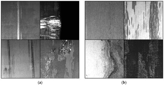
Figure 2.
Examples of surface scratches and abrasions (a) and undamaged surfaces (b).
3.3. Model Quality Metrics
The metric—Dice similarity coefficient—was used to assess the segmentation quality (Figure 3a). The metric—Intersection over Union—was calculated to compare the segmentation results with those obtained by other authors (Figure 3b):
where is the actual damage object according to the marking, and is the damage object obtained after segmentation.
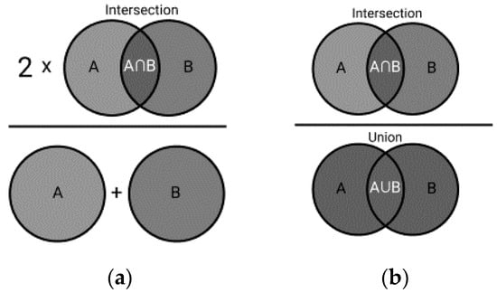
Figure 3.
Calculation of segmentation quality metrics: Dice similarity coefficient (a) and Intersection over Union (b).
The following expression was used to calculate :
where is the addend used to prevent division by zero.
is the array of integers, where 0 denotes the background pixel, and 1 indicates the damage pixel. From the original sigmoid neurons of the original layer, we obtain real values in the range of . When testing after thresholding, will also contain integers. However, the optimal threshold is unknown during training. Therefore, will contain valid values, resulting in a smaller metric value.
Since the output values of the neural network are in the range of , the best similarity metrics, and , were calculated for different quality thresholds.
Apart from the and metrics, we used metrics to evaluate the binary classification of pixels into classes (defect–not defect): , , .
The recall metric shows what part of pixels that belong to damage is recognized correctly:
The precision metric demonstrates which part of pixels that belong to damage is recognized as actually belonging to damage:
The score is an integrated metric and can be interpreted as a weighted average of the precision and recall, where the score attains its best score at 1 and worst score at 0. The relative contributions of precision and recall to the score are equal:
3.4. Investigated Neural Network Optimizers
A neural network optimizer is an algorithm or method used to change neural network parameters, such as neuron weights, to achieve the lowest loss. The optimizer implements the loss reduction strategy and allows achieving the most accurate result.
Since the choice of optimizer is important and can significantly affect the final accuracy of segmentation, we investigated several optimization algorithms: SGD, Adagrad, Adadelta, RMSprop and Adam.
3.4.1. Stochastic Gradient Descent (SGD)
SGD is an iterative method for optimizing the loss function with pre-set smoothing properties. SGD allows minimizing the loss function J (θ) parameterized by the model weights using the backward update of parameters with respect to the gradient of the loss function . The learning rate η determines the step size in the local minimum direction. Thus, we move in the surface slope direction set by the loss function until we reach the minimum. In this case, model weights are updated after calculating losses for each input sample with a mark :
However, the original SGD algorithm has difficulty in navigating those parts of the loss function surface where the surface bend in one dimension is much steeper than in another. Therefore, we also used the Nesterov momentum method, which allows accelerating the optimizer in the right direction and eliminates the fluctuations in the loss function. This is conducted by adding the fraction of the increment vector of the previous step to the expected future parameter vector.
When training models with the SGD optimizer, was used.
The Nesterov-accelerated gradient first jumps in the direction of the previous accumulated gradient, measures the gradient and then corrects the complete parameter update. This anticipatory update prevents going too fast and results in increased responsiveness, which significantly increases the performance of the neural network [38].
The stochastic gradient method is one of the most commonly used methods for optimization in the training of deep neural networks [39,40,41]. However, the disadvantage of this algorithm consists in the noticeable effect of the learning rate on finding the best model. An improperly selected learning rate can lead to suboptimal increases in parameters during training. Therefore, they often use optimizers, which automatically adjust the learning rate to the loss function gradient.
3.4.2. Adagrad
This gradient algorithm adjusts the learning rate to the parameters. As a result, a smaller increment is provided for the parameters associated with common features, and a larger increment is provided for the parameters associated with infrequent features. This optimizer has proven itself sufficient in solving many practical problems [42].
The diagonal matrix is used when calculating neural network parameters. In this matrix, each diagonal element is the sum of gradient squares for the parameter prior to step :
where is the leveling value, which does not allow division by zero: as a rule, ; is the gradient value for step .
One of the main advantages of the Adagrad algorithm is that it eliminates the need to manually adjust the learning rate. Most of its realizations use the default value of 0.01 and leave it. The main disadvantage of Adagrad is the accumulation of gradient squares in the denominator: since each addend is positive, the accumulated amount keeps growing during training. This, in turn, reduces the learning rate, which eventually becomes infinitesimally small. After that, the algorithm can no longer receive additional knowledge.
3.4.3. Adadelta
This is an advanced version of Adagrad: instead of accumulating all previous gradients, Adadelta restricts the accumulation of gradients to a window with a certain fixed size.
where is the operator of the root mean squared error.
The Adadelta optimizer does not even need to set the default learning rate, since it is excluded from the parameter update equation.
3.4.4. RMSprop
Like Adadelta, this optimizer attempts to solve the problem faced by Adagrad, which consists in the learning rate being decreased to a level at which further acquisition of knowledge by the neural network is impossible. RMSprop also divides the learning rate by an exponentially decaying average of squared gradients.
3.4.5. Adam
The Adaptive Moment Estimation calculates the adaptive learning rate for each parameter. In addition to maintaining an exponentially decreasing mean value of the past gradient squares, Adam, in line with Adadelta and RMSprop, maintains an exponentially decreasing mean value of the past gradients, which is similar to the moment approach. The equation for updating parameters during training is similar to RMSprop:
where and are the evaluation of the first and second moments, respectively.
4. Experiment and Discussion
4.1. Training Neural Network Model for Segmentation
For the neural network not to start detecting signs at random, we used the transfer learning technique. To do this, the neural network was previously initialized by weights obtained during training based on ImageNet images, which in total include more than 1.4 million images divided into 1000 different classes.
When conducting training on input images larger than 256 × 256 pixels, areas of 256 × 256 pixels were randomly selected (according to the input layer size), from which the tensor fed to the neural network input was formed. In addition, each frame cut off the image was randomly transformed (horizontal and vertical flip, rotation by an angle multiple of 90°). As part of solving the classification problem, previous studies have also shown that augmentation allows achieving a better performance of the model [24,25,26]. The approach used has significantly diversified training data and created the conditions under which training batches are never repeated in practice. This approach was used in both the neural network training and validation. This allowed training the model on an extended dataset, as well as validating the result of learning on dynamically generated data.
Neural network segmentation models were implemented in Python 3.8 using the TensorFlow and Keras libraries, version 2.6.0. A workstation based on Intel Core and a 7-2600 CPU, 32 GiB RAM and two NVIDIA GeForce GTX 1060 GPUs with 6 GiB of video memory was used for training and testing.
When training the neural network, its parameters were saved after each training epoch. When the loss function did not decrease over the previous 10 epochs, the learning rate was reduced by 20%. At the end of each epoch, the model was saved, as well as the training and validation quality metrics, such as DSC, IoU, precision, recall and F1-score. Training of a model was discontinued when the learning rate became less than 0.0001, or when the loss function did not improve its value over 20 epochs.
4.2. Investigation of Optimizers
There are many different studies in the field of image defect recognition, in which the authors used different optimization techniques. In [39,40,41,42], the SGD algorithm was used, and good quality metrics were achieved. Dong [43] and Jiang [44] used the Adam optimizer to train a semantic segmentation model and also reported good results. Liu et al. [45] used the SGD and Adam optimizers for training R-CNN-based object recognition models. In both cases, the results were good, but slightly better results were achieved using the Adam optimizer.
Although adaptive optimization methods have a number of advantages over the “traditional” SGD algorithm, and their use is becoming more common, they often account for the impaired generalization properties of the model [46]. In addition, Adam is unable to find a minimum loss function in some cases [47].
To study the optimizer’s influence on the final result of training the neural network, a number of experiments were conducted, in which a neural network with a certain architecture was trained on the same images, but with different optimizers. Next, the neural networks obtained were tested on images by calculating the test quality metrics. Training with each optimizer was performed three times. After that, the best result was selected.
Figure 4 shows the results of damage recognition on the test set of images obtained for the U-Net segmentation model with a ResNet152 backbone. The highest values of the and metrics were attained when training the model using the SGD optimizer with Nesterov momentum (SGD + in Figure 4). SGD without momentum (SGD- in Figure 4) showed a much worse result. Another good result, although slightly worse, was attained when training the model using the Adagrad and Adam optimizers. The worst results were obtained using the RMSprop and Adadelta optimizers.
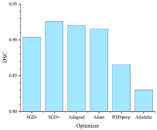
Figure 4.
Accuracy of damage detection on test images depending on the optimizer selected during the training of the U-Net neural network with a ResNet152 backbone.
Thus, in the context of our problem, the best results were achieved when training models using the SGD optimizer with Nesterov momentum and the learning rate selected manually. Almost the same results were obtained using the Adagrad technique. Based on the results of a preliminary study, the algorithm for optimizing SGD training with Nesterov momentum was selected for further application.
The advantages of stochastic gradient descent are efficiency, lots of opportunities for tuning and (for larger datasets) faster convergence as it causes updates to the parameters more frequently. Therefore, even though SGD has been used in machine learning tasks for a long time, it has attracted a considerable amount of attention recently in the context of large-scale learning [46,47].
4.3. Relation between Validation and Test Metrics
Another issue to be addressed in the training of the neural network model is the model sampling after the appropriate training cycles according to their validation metrics. The fact is that no unambiguous relationship exists between the validation and test metrics. Therefore, the model that demonstrates the best validation performance is not always the best one when applied to test data.
In the process of the neural network training after each epoch, we have a model with some validation metrics. However, different metrics often do not agree with each other, and the model can show a good value of one of the metrics and, at the same time, a much worse value of another. As practice shows, the highest value of the validation metric is not always an indication that the model will be better when applied to test data.
Therefore, it is important to choose the model state that will correspond to the best results on the test data, which is currently unresolved.
After each training epoch, the model was validated, and the loss functions were recorded, as well as the , , , and metrics. To study the dependence of the main quality metric—the DSC test value—on the validation parameters listed, was calculated for several segmentation models saved during training. After that, the correlation coefficient between and all validation parameters was calculated (see Table 1).

Table 1.
Correlation between and validation metrics for the U-Net model with a ResNet152 backbone.
As expected, the highest correlation was found between pairs and . Interestingly, the pixel-by-pixel metrics and were in themselves less correlated with , but the integrated metric calculated on their basis was also significantly correlated with the test metric. The loss function was also markedly (inversely) correlated with , although to a lesser extent.
Thus, based on the previous study, the metrics were used to select models during training. Models characterized by the three best values of each metric were selected for further study (for —maximum values; for —minimal values) after investigating the neural network segmentation model.
4.4. Comparing Models of Different Architectures and Choosing the Best One
To develop a model for recognizing damage such as “scratch abrasion” according to the method described above, a number of neural networks with the U-Net architecture, but different backbones, were trained. During the training of the same model on the same data, different recognition results can be obtained. Therefore, each model was trained from scratch three times, and for the final rating, we chose the one that showed the best result.
The SGD optimizer, learning rate , binary cross-entropy loss function and batch size 12 were used for training. Each model was tested on test images. Since the sigmoid activation function was used in the source layer of the classifier, the output value for each pixel was in the range of . This value can be interpreted as the degree of model confidence in the affiliation of a given pixel in the image to the defect, or as the defect severity: less noticeable defects usually correspond to smaller values, and vice versa. The final decision on the presence of damage is made if the output neuron value exceeds a certain threshold. Since the test metrics depend on the value of this threshold, they were calculated for a number of thresholds from 0.30 to 0.80, and the best one was chosen. The dependence of the metric on the threshold is shown in Figure 5a. Most of the maxima fall on the average range from 0.50 to 0.65, which indicates that the model adjusted to specimens provided during training. Comparative validation metrics of the same models are shown in Figure 5b.
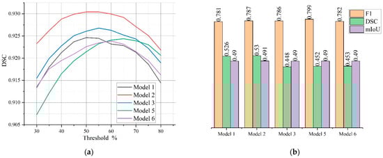
Figure 5.
Dependence of the test metric on threshold values of the output layer (a) and values of the validation metrics , and for different models (b).
Comparative results for models of different architectures are presented in Table 2. For models of each architecture, the best values obtained at the optimal threshold value were selected.
Table 2.
Summary table of the test metrics DSC and IoU for models of different architectures.
The best results were consistently demonstrated by U-Net models with ResNet and DenseNet backbones of different depths. Networks based on the SeResNet, SeResNeXt, ResNeXt and Inception architectures performed slightly worse. EfficientNet and MobileNet, which have a lower depth and focus primarily in mobile and embedded systems, showed the lowest accuracy in defect recognition, as expected.
Neural networks with a number of layers up to 100 had an insufficient generalization ability to accumulate feature maps necessary for the successful detection of defects (on the studied dataset). Neural networks with a large number of layers (above 200), having good validation metrics, demonstrated worse results on the test data. This is probably due to the effect of overtraining and the deterioration of their generalization capabilities.
The MobileNet and EfficientNet neural networks are more focused on fast data processing; they not only contain fewer layers but also use normalization techniques. This allows them to train faster, but due to the averaging of the model parameters in some cases, this leads to worse accuracy metrics. Therefore, such models usually have a good ratio of “learning speed/accuracy”, but compared to more complex models, they have a poorer detection quality.
The model with the highest accuracy of the test dataset was selected as the final one. The best results were achieved with the U-Net—ResNet model with an encoder depth of 152 layers. The test metrics of this model were , and . The training dynamics of model 2 (see Table 2) are shown in Figure 6. Since the optimal threshold value was unknown during training, the and metrics were calculated based on the current valid values of the source layer. Therefore, the value of the validation metrics was significantly lower than the final metric obtained from the test data. The graphs demonstrate a gradual training process; however, the indicators reached a certain limit and practically did not change after about 100 epochs. Model 2 was obtained after 118 epochs of training.
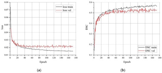
Figure 6.
Loss function (a) and metric (b) when training model 2.
4.5. Defect Detection Using the Model Developed
The image of the test dataset was investigated using the model developed. In general, the model was found to accurately reproduce the position and shape of damage in the images. Figure 7a,b visualize the results obtained for the neural network output layer (model 2) when recognizing defects such as “scratch abrasion”. As seen, the proposed model was good at recognizing individual linear defects, their groups and scratched areas with chaotic non-linear defects. At the same time, the output layer value (defect brightness in Figure 7b,d,f) corresponds to the clarity and contrast of the defect in the input image. Less pronounced defects correspond to a slightly weaker intensity of the area at the output.
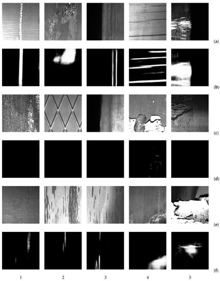
Figure 7.
Examples of test images with damage such as “scratch abrasion” (a), and the results of their recognition using model 2 (b); examples of defect-free surfaces (c), and the result of their recognition (d); examples of erroneous recognition of defects (e,f).
Surfaces that do not contain defects such as “scratch abrasion” were also well recognized, regardless of the complex surface formations (Figure 7c,d). Low-intensity artifacts are sometimes found on the source layer for such images; however, they are easy to discard by thresholding.
However, erroneous recognition is also common (Figure 7e,f). It may occur in cases where:
Expert analysis of the defect detection results showed that mostly false positive cases of recognition are related to areas that are similar in shape, texture or color to the real damage. Probably, the number of false positives can be reduced by expanding the training dataset with images containing such defects.
Most false negative cases are related to unnoticeable minor defects.
To compare the accuracy of the model developed with similar methods developed by other authors, the quality metrics of different models are summarized in Table 3. It is obvious that the model metrics intended for solving completely different problems cannot be compared accurately. Model metrics depend on the training data type, their noise level, the number of defect classes, quick response requirements, etc. However, our results are similar to those attained by other authors in similar areas under real industrial conditions.
Table 3.
Test metrics of the developed model as compared to metrics of similar models for surface damage detection.
In addition to localizing damage on the surface studied, segmented images allow obtaining its quantitative description and calculating its geometric parameters (area, length, width, slope, diameter, etc.) [48,49,50]. This is an important task, but it is outside the scope of our current work.
5. Conclusions
We developed and researched 14 neural network models for defect detection on metal surfaces. U-Net-like architectures with encoders such as ResNet, SEResNet, SEResNeXt, DenseNet, InceptionV3, Inception-ResNetV2, MobileNet and EfficientNet were investigated as part of the problem, which consisted in detecting defects such as “scratch abrasion”.
Recognition accuracy was analyzed as affected by the optimizer during neural network training. In the context of this problem, neural networks trained using the stochastic gradient descent optimizer with Nesterov momentum were found to have the best generalizing properties. The highest metrics of the Dice similarity coefficient were obtained for these neural networks. A good result was also attained using the Adagrad optimizer.
The main test metric of recognition quality () was analyzed as depending on the validation metrics to provide for a better selection of the best model during its training based on the validation metrics. The validation metrics were found to be the most correlated with the metric.
The ResNet and DenseNet models with a depth of 50 layers showed the best generalizing properties. The highest recognition accuracy was attained using the U-Net model with a ResNet152 backbone. On the test dataset, the result obtained using this model was and . Thus, the proposed training method allowed us to obtain results similar to those provided for by the state-of-the-art models used for defect detection.
Semantic segmentation is the first important step to identify damaged areas on metal surfaces. However, from the point of view of defectometry, the quantitative assessment of damaged surfaces is also important. Segmentation makes it possible to calculate damage parameters such as the area, linear dimensions, shape and slope, as well as fractal characteristics and texture. These issues remain outside the scope of our current study, and we intend to explore them in future work.
Author Contributions
This research was conceptualized by I.K., P.M. and O.P.; the experiments (investigation) were conducted by I.K. and P.M.; the simulations using software were performed by J.B. (Jakub Brezina); and the results (formal analysis) were analyzed and discussed by I.K., P.M. and J.B. (Janette Brezinová) The manuscript was written (original draft) by I.K., P.M., J.B. (Janette Brezinová) and J.B. (Jakub Brezina) and reviewed (writing and editing) by O.P. All authors have read and agreed to the published version of the manuscript.
Funding
This research was funded by the Scientific Grant Agency, “Application of progressive technologies in restoration of functional surfaces of products” (1/0497/20), the Cultural and Educational Grant Agency, “Modernization of teaching in the field of technologies for joining construction materials” (001STU-4/2019), and the Slovak Research and Development Agency APVV-20-0303, “Innovative approaches to the restoration of functional surfaces by laser weld overlaying”.
Institutional Review Board Statement
Not applicable.
Informed Consent Statement
Not applicable.
Data Availability Statement
The data presented in this study are available upon request from the corresponding author.
Acknowledgments
The research described in this paper was financially supported by the Scientific Grant Agency, “Application of progressive technologies in restoration of functional surfaces of products” (1/0497/20), and the Cultural and Educational Grant Agency, “Modernization of teaching in the field of technologies for joining construction materials” (001STU-4/2019). This support is highly appreciated by the authors.
Conflicts of Interest
The authors declare no conflict of interest.
References
- Pimenov, V.A.; Kopylov, A.F.; Glebov, V.P.; Kononykhin, G.N. Effect of the form of the narrow faces of slabs and their deformation during hot rolling on the topography of surface defects on the finished rolled product. Metallurgist 2015, 58, 784–787. [Google Scholar] [CrossRef]
- Pimenov, V.A.; Dagman, A.I.; Pogodaev, A.K.; Kovalev, D.A.; Zhovnodii, N.N. Surface finish enhancement of hot-rolled strips on the 2000 wide-strip rolling mill using mathematical modeling at Novolipetsk Steel. Steel Transl. 2019, 49, 703–708. [Google Scholar] [CrossRef]
- Pimenov, V.A.; Dagman, A.I.; Kovalev, D.A. Analysis and mathematical simulation of formation regularities of strip transversal profile during hot rolling. Steel Transl. 2020, 50, 107–111. [Google Scholar] [CrossRef]
- Bolobanova, N.L.; Garber, E.A. Study and modeling of slab deformation processes in the roughing stands of Severstal’s Mill-2000 hot-rolling line. Metallurgist 2012, 65, 564–570. [Google Scholar] [CrossRef]
- Luo, Q.; Fang, X.; Liu, L.; Yang, C.; Sun, Y. Automated visual defect detection for flat steel surface: A Survey. IEEE Trans. Instrum. Meas. 2020, 69, 626–644. [Google Scholar] [CrossRef] [Green Version]
- Markulik, S.; Nagyova, A.; Turisova, R.; Villinsky, T. Improving quality in the process of hot rolling of steel sheets. Appl. Sci. 2021, 11, 5451. [Google Scholar] [CrossRef]
- Litvintseva, A.; Evstafev, O.; Shavetov, S. Real-time steel surface defect recognition based on CNN. In Proceedings of the IEEE 17th International Conference on Automation Science and Engineering (CASE), Lyon, France, 23–27 August 2021; pp. 1118–1123. [Google Scholar] [CrossRef]
- Damacharla, P.; Rao, A.; Ringenberg, J.; Javaid, A.Y. TLU-Net: A deep learning approach for automatic steel surface defect detection. In Proceedings of the International Conference Applied Artificial Intelligence (ICAPAI), Halden, Norway, 19–21 May 2021; pp. 1–6. [Google Scholar]
- Prihatno, A.T.; Utama IB, K.Y.; Kim, J.Y.; Jang, Y.M. Metal defect classification using deep learning. In Proceedings of the Twelfth International Conference on Ubiquitous and Future Networks (ICUFN), Jeju Island, Korea, 17–20 August 2021; pp. 389–393. [Google Scholar]
- Zhou, S.; Liu, H.; Cui, K.; Hao, Z. JCS: An Explainable Surface Defects Detection Method for Steel Sheet by Joint Classification and Segmentation. IEEE Access 2021, 9, 140116–140135. [Google Scholar] [CrossRef]
- Neven, R.; Goedemé, T. A Multi-branch U-Net for steel surface defect type and severity segmentation. Metals 2021, 11, 870. [Google Scholar] [CrossRef]
- Tao, X.; Zhang, D.; Ma, W.; Liu, X.; Xu, D. Automatic metallic surface defect detection and recognition with convolutional neural networks. Appl. Sci. 2018, 8, 1575. [Google Scholar] [CrossRef] [Green Version]
- Aslam, Y.; Santhi, N.; Ramasamy, N.; Ramar, K. Localization and segmentation of metal cracks using deep learning. J. Ambient Intell. Humaniz. Comput. 2020, 12, 4205–4213. [Google Scholar] [CrossRef]
- Qian, K. Automated Detection of steel defects via machine learning based on real-time semantic segmentation. In Proceedings of the 3rd International Conference on Video and Image Processing (ICVIP 2019). Association for Computing Machinery, New York, NY, USA, 20–23 December 2019; pp. 42–46. [Google Scholar] [CrossRef]
- Yu, H.; Li, X.; Song, K.; Shang, E.; Liu, H.; Yan, Y. Adaptive depth and receptive field selection network for defect semantic segmentation on castings X-rays. NDT E Int. 2020, 116, 102345. [Google Scholar] [CrossRef]
- Zhu, Y.; Yang, R.; He, Y.; Ma, J.; Guo, H.; Yang, Y.; Zhang, L. A Lightweight multiscale attention semantic segmentation algorithm for detecting laser welding defects on safety vent of power battery. IEEE Access 2021, 9, 39245–39254. [Google Scholar] [CrossRef]
- Kim, H.; Lee, S.; Han, S. Railroad Surface Defect Segmentation Using a Modified Fully Convolutional Network. KSII Trans. Internet Inf. Syst. 2020, 14, 4763–4775. [Google Scholar] [CrossRef]
- Ronneberger, O.; Fischer, P.; Brox, T. U-Net: Convolutional networks for biomedical image segmentation. In Medical Image Computing and Computer—Assisted Intervention 2015; Navab, N., Hornegger, J., Wells, W.M., Frangi, A.F., Eds.; Springer International Publishing: Cham, Switzerland, 2015; pp. 234–241. [Google Scholar]
- Guan, S.; Khan, A.A.; Sikdar, S.; Chitnis, P.V. Fully Dense UNet for 2-D sparse photoacoustic tomography artifact removal. IEEE J. Biomed. Health Inform. 2020, 24, 568–576. [Google Scholar] [CrossRef] [PubMed] [Green Version]
- Huang, H.; Lin, L.; Tong, R.; Hu, H.; Zhang, Q.; Iwamoto, Y.; Han, X.; Chen, Y.-W.; Wu, J. UNet 3+: A Full-Scale Connected UNet for Medical Image Segmentation. Proceedngs of the ICASSP 2020—2020 IEEE International Conference on Acoustics, Speech and Signal Processing (ICASSP), Barcelona, Spain, 4–8 May 2020; pp. 1055–1059. [Google Scholar] [CrossRef]
- Enshaei, N.; Ahmad, S.; Naderkhani, F. Automated detection of textured-surface defects using UNet-based semantic segmentation network. In Proceedings of the IEEE International Conference on Prognostics and Health Management (ICPHM), Detroit, Michigan, 8–10 June 2020; pp. 1–5. [Google Scholar] [CrossRef]
- Üzen, H.; Türkoğlu, M.; Hanbay, D. Surface defect detection using deep U-net network architectures. In Proceedings of the 29th Signal Processing and Communications Applications Conference (SIU), Istanbul, Turkey, 9–11 June 2021; pp. 1–4. [Google Scholar] [CrossRef]
- Choi, S. Traffic map prediction using UNet based deep convolutional neural network. arXiv 2019, arXiv:1912.05288v1. [Google Scholar]
- Konovalenko, I.; Maruschak, P.; Brezinová, J.; Viňáš, J.; Brezina, J. Steel surface defect classification using deep residual neural network. Metals 2020, 10, 846. [Google Scholar] [CrossRef]
- Konovalenko, I.; Maruschak, P.; Brevus, V.; Prentkovskis, O. Recognition of scratches and abrasions on metal surfaces using a classifier based on a convolutional neural network. Metals 2021, 11, 549. [Google Scholar] [CrossRef]
- Konovalenko, I.; Maruschak, P.; Brevus, V. Steel surface defect detection using an ensemble of deep residual neural networks. J. Comput. Inf. Sci. Eng. 2022, 22, 014501. [Google Scholar] [CrossRef]
- He, K.; Zhang, X.; Ren, S.; Sun, J. Deep residual learning for image recognition. In Proceedings of the 2016 IEEE Conference on Computer Vision and Pattern Recognition (CVPR), Las Vegas, NV, USA, 26 June–1 July 2016; pp. 770–778. [Google Scholar] [CrossRef] [Green Version]
- Hu, J.; Shen, L.; Albanie, S.; Sun, G.; Wu, E. Squeeze-and-Excitation Networks. arXiv 2019, arXiv:1709.01507v4. [Google Scholar]
- Huang, G.; Liu, Z.; van der Maaten, L.; Weinberger, K.Q. Densely Connected Convolutional Networks. arXiv 2018, arXiv:1608.06993v5. [Google Scholar]
- Szegedy, C.; Liu, W.; Jia, Y.; Sermanet, P.; Reed, S.; Anguelov, D.; Erhan, D.; Vanhoucke, V.; Rabinovich, A. Going Deeper with Convolutions. arXiv 2014, arXiv:1409.4842v1. [Google Scholar]
- Szegedy, C.; Vanhoucke, V.; Ioffe, S.; Shlens, J.; Wojna, Z. Rethinking the inception architecture for computer vision. arXiv 2015, arXiv:1512.00567v3. [Google Scholar]
- Szegedy, C.; Ioffe, S.; Vanhoucke, V.; Alemi, A. Inception-v4, Inception-ResNet and the Impact of Residual Connections on Learning. arXiv 2016, arXiv:1602.07261v2. [Google Scholar]
- Howard, A.G.; Zhu, M.; Chen, B.; Kalenichenko, D.; Wang, W.; Weyand, T.; Andreetto, M.; Adam, H. MobileNets: Efficient Convolutional Neural Networks for Mobile Vision Applications. arXiv 2017, arXiv:1704.04861v1. [Google Scholar]
- Tan, M.; Le, Q.V. EfficientNet: Rethinking Model Scaling for Convolutional Neural Networks. arXiv 2019, arXiv:1905.11946v5. [Google Scholar]
- Deng, J.; Dong, W.; Socher, R.; Li, L.-J.; Li, K.; Fei-Fei, L. ImageNet: A large-scale hierarchical image database. In Proceedings of the 2009 IEEE Conference on Computer Vision and Pattern Recognition, Miami, FL, USA, 20–25 June 2009; pp. 248–255. [Google Scholar] [CrossRef] [Green Version]
- Lin, T.Y.; Maire, M.; Belongie, S.; Bourdev, L.; Girshick, R.; Hays, J.; Perona, P.; Zitnick, C.L.; Dollár, P. Microsoft COCO: Common Objects in Context. arXiv 2014, arXiv:1405.0312v3. [Google Scholar]
- Kaggle Severstal: Steel Defect Detection. Can You Detect and Classify Defects in Steel? 2019. Available online: https://www.kaggle.com/c/severstal-steel-defect-detection (accessed on 23 November 2021).
- Bengio, Y.; Boulanger-Lewandowski, N.; Pascanu, R. Advances in Optimizing Recurrent Networks. arXiv 2012, arXiv:1212.0901v2 [cs.LG]. [Google Scholar]
- Li, Y.; Huang, H.; Xie, Q.; Yao, L.; Chen, Q. Research on a Surface Defect Detection Algorithm Based on MobileNet-SSD. Appl. Sci. 2018, 8, 1678. [Google Scholar] [CrossRef] [Green Version]
- Liyun, X.; Boyu, L.; Hong, M.; Xingzhong, L. Improved Faster R-CNN algorithm for defect detection in powertrain assembly line. Procedia CIRP 2020, 93, 479–484. [Google Scholar] [CrossRef]
- Ferguson, M.K.; Ronay, A.; Lee, Y.T.; Law, K.H. Detection and segmentation of manufacturing defects with convolutional neural networks and transfer learning. Smart Sustain. Manuf. Syst. 2018, 2, 1007121126. [Google Scholar] [CrossRef]
- Mao, M.; Ranzato, M.; Senior, A.; Tucker, P.; Yang, K.; Le, Q.; Ng, A. Large scale distributed deep networks. In Proceedings of the NIPS 2012: Neural Information Processing Systems, Lake Tahoe Nevada, CA, USA, 3–6 December 2012; pp. 1–11. [Google Scholar]
- Dong, X.; Taylor, C.J.; Cootes, T.F. Small Defect Detection Using Convolutional Neural Network Features and Random Forests; Leal-Taixé, L., Roth, S., Eds.; Computer Vision—ECCV 2018 Workshops. ECCV 2018. Lecture Notes in Computer Science; Springer: Cham, Switzerland, 2019; p. 11132. [Google Scholar] [CrossRef]
- Jiang, Q.; Tan, D.; Li, Y.; Ji, S.; Cai, C.; Zheng, Q. Object detection and classification of metal polishing shaft surface defects based on convolutional neural network deep learning. Appl. Sci. 2020, 10, 87. [Google Scholar] [CrossRef] [Green Version]
- Liu, M.-W.; Lin, Y.-H.; Lo, Y.-C.; Shih, C.-H.; Lin, P.-C. Defect detection of grinded and polished workpieces using faster R-CNN. In Proceedings of the IEEE/ASME International Conference on Advanced Intelligent Mechatronics (AIM), Delft, The Netherlands, 12–16 July 2021; pp. 1290–1296. [Google Scholar] [CrossRef]
- Zhou, P.; Feng, J.; Ma, C.; Xiong, C.; Hoi, S.; Weinan, E. Towards Theoretically Understanding Why SGD Generalizes Better Than ADAM in Deep Learning. arXiv 2020, arXiv:2010.05627v1. [Google Scholar]
- Reddi, S.J.; Kale, S.; Kumar, S. On the convergence of adam and beyond. arXiv 2019, arXiv:1904.09237v1. [Google Scholar]
- Konovalenko, I.; Hutsaylyuk, V.; Maruschak, P. Classification of surface defects of rolled metal using deep neural network ResNet50. In Proceedings of the 13th International Conference on Intelligent Technologies in Logistics and Mechatronics Systems, Panevezys, Lithuania, 1 October 2020; pp. 41–48. [Google Scholar]
- Konovalenko, I.; Maruschak, P.; Kozbur, H.; Brezinová, J.; Brezina, J.; Guzanová, A. Defectoscopic and geometric features of defects that occur in sheet metal and their description based on statistical analysis. Metals 2021, 11, 1851. [Google Scholar] [CrossRef]
- Konovalenko, I.; Maruschak, P.; Kozbur, H.; Brezinová, J.; Brezina, J.; Nazarevich, B.; Shkira, Y. Influence of uneven lighting on quantitative indicators of surface defects. Machines 2022, 10, 194. [Google Scholar] [CrossRef]
Publisher’s Note: MDPI stays neutral with regard to jurisdictional claims in published maps and institutional affiliations. |
© 2022 by the authors. Licensee MDPI, Basel, Switzerland. This article is an open access article distributed under the terms and conditions of the Creative Commons Attribution (CC BY) license (https://creativecommons.org/licenses/by/4.0/).