A New Framework for the Harmonic Balance Method in OpenFOAM

Abstract

The Harmonic Balance Method is one of the most commonly employed Reduced Order Models for turbomachinery calculations, since it leverages the signal sparsity in the frequency domain to cast the transient equations into a coupled set of steady-state ones. The present work aims at detailing the development and validation of a new framework for the application of the Harmonic Balance Method in the open-source software OpenFOAM. The paper is conceptually divided into building blocks for the implementation of the code. For each of these, theoretical notions and coding strategies are given, and an ad hoc validation test case is presented. This structure has been chosen with the aim of easing the reader in the understanding and implementation of such a method in a generic fluid dynamics solver. In a fully open source philosophy, the library files are freely accessible in the authors’ repository (link provided below in the text).

1. Introduction

Computational Fluid Dynamics (CFD) has become a landmark for academics and industries to analyze the flow field behaviour in complex domains. Part of its success is inherently due to CFD capacity of keeping pace with the increasingly demanding requirements of the scientific community in terms of performance and accuracy. Several challenges still remain about the simulation of large multi-scale domains, though. One striking example of such occurrence is the efficient simulation of unsteady turbulent flows in multi-stage turbomachinery. Time-domain solvers are still the most commonly employed, although they tend to be very computationally demanding. One of the methods CFD engineers and computer scientists are tackling these problems with, is the development of efficient algorithms to embed complex flow fields into a low-dimensional space (i.e., Reduced Order Models (ROMs)). Among ROMs, the Harmonic Balance Method (HBM) has established as a state-of-the-art tool for the calculation of periodic and quasi-periodic flows in time. While conventional Unsteady Reynolds Averaged Simulations (URANS) and Large Eddy Simulations (LES) can capture unsteady phenomena occurring at non-deterministic frequencies (e.g., vortex shedding), turbulent aeroacoustics interactions and transient non-periodic flows, many turbomachinery applications of interest exhibit periodic oscillations at known frequencies. In these cases, the HBM can be applied, resulting in a drop in computational time of typically one/two orders of magnitude compared to URANS analysis. It is evident that this could have a profound impact, especially in the design phase, when one may want to conduct a large number of calculations at a reduced cost to explore the design space, but unsteady phenomena still play an important role and must be accounted for. A thorough review of the numerical methods commonly employed for turbomachinery calculations with different levels of fidelity, including LES and hybrid methods, can be found in Tucker [1,2]. Compared to other ROMs, the HBM has the advantage of exploiting a universal basis (i.e., the Fourier basis) for the projection of the governing equation and therefore does not require any previous experimental or numerical data produced by the system. On the contrary, data-driven methods, such as the Proper Orthogonal Decomposition (POD) [3], employ a problem-dependent basis tailored on the specific dataset analyzed which will be optimal in representing the data in a desired sense. It is worth noticing that, as for every other ROM, the accuracy of the HBM is highly dependent on the number of non-zero entries retained in the chosen basis.

The HBM method originates from the ideas of He [4] and Hall [5] of leveraging the known spectral content of the flow to cast the equations into the frequency domain. In this way, the signal sparsity in the Fourier basis is exploited to approximate the time derivative in the governing equations. Applications of this method are manifold and range from limit cycle oscillation of aerodynamic components [6] to forced response problem in multi-row turbomachinery [7]. In the literature, many authors report different implementations of the method and its application to diverse problems. Hall et al. [5] and Thomas et al. [8] investigated the aerodynamics effects on flutter of a transonic compressor rotor and of airfoils, respectively. Jameson et al. [9] used a similar non-linear frequency domain method to study vortex shedding behind a cylinder and a pitching airfoil. They also modified their method that iteratively solves for the time period during the solution of the Navier–Stokes equations. van der Weide et al. [10] used their Time Spectral Method implemented in the TFLO2000 solver to compute the forced response in an axial compressor stage. One drawback of their method was that they had to use the same number of blades for the stator and the rotor. To overcome this issue, Ekici et al. [7] extended the harmonic balance technique to multi-stage turbomachinery employing a multi-frequencial HBM, where excitations at frequencies non-harmonically related to each other were considered. Later on, Gopinath et al. [11] and Sicot et al. [12] used a time-domain approach for inter-row coupling in axial compressors. Furthermore, Su and Yuan [13], Woodgate and Badcock [14], Sicot et al. [15] and Thomas et al. [16] proposed different implicit formulations of the HBM. More recently, Frey et al. proposed a frequency-domain formulation for multi-stage turbomachinery and implemented it in the TRACE solver. Nimmagaddda et al. [17] implemented an explicit version of the HBM in the open-source software SU2 and tested it on a pitching airfoil with multiple oscillation frequencies. Finally, Cvijetic et al. [18] and Oliani et al. [19] proposed a pressure-based HBM formulation for incompressible flows using foam-extend and OpenFOAM, respectively. In these works, an explicit formulation was used for the discretization of the source terms arising from the application of the HBM. On the contrary, in this paper we develop a novel density-based solver suitable for compressible, high-speed turbomachinery calculations and employ a fully-implicit formulation which significantly enhances the stability and convergence properties of the calculations. In addition, phase-lag boundary conditions allowing for single passage reduction were implemented, further speeding up the calculation. For a thorough review on the HBM and its variants, the reader is referred to the works of Hall et al. [20] and He [21].

The outline of the paper is as follows. In the next sections, the governing equations and the mathematical formulation of the HBM are illustrated. The implementation of a fully implicit HBM in the OpenFOAM (OF) framework, starting from the baseline formulation for a single fundamental frequency and its harmonics, is described. Attention is focused on the numerical solution of the resultant equation system and the related CFD code. We then move to more complex issues such as the multi-frequential formulation and the use of phase-lag boundary condition to reduce the computational domain to a single blade passage per row. For each step, the critical algorithmic issues are discussed, and the pseudo-code for the implementation is detailed. One of the main aims is to provide the reader with a thorough understanding of the building blocks necessary for the coding of a harmonic balance technique.

Furthermore, this work introduces several sources of novelty with respect to the state of the art. To begin with, this is the first implementation of a fully implicit HBM in a density-based solver in the context of open-source CFD softwares. We also illustrate how geometries with a rotational periodicity must be carefully treated when solving the equations in cartesian coordinates instead of cylindrical ones. Furthermore, we show how coupled interfaces typical of turbomachinery simulations can be integrated in the OF framework in an simple way. Additionally, as will be detailed in the next section, the very use of implicit density-based solvers in OF has been extremely limited so far, especially with respect to multi-row turbomachinery applications. All this being considered, the present work aims to represent a step forward in the growing application of open-source codes to industrial problems. Given also the wide diffusion of the C++ library OpenFOAM, the research community could benefit from this work as a starting point to enrich the current capabilites of the code with frequency domain methods for turbomachinery.

The code is available in the authors’ repository: https://github.com/stefanoOliani/ICSFoam (accessed on 3 March 2022), and can be freely shared, edited and distributed by the users.

2. Implicit Density-Based Solver Implementation

2.1. Governing Equations

In the present work, we solve the unsteady three-dimensional compressible Reynolds-averaged Navier–Stokes (RANS) equations in conservation form:

$${\int }_V\frac{\partial \mathbf{Q}}{\partial t}dV+{\int }_{\partial V}\left({\mathit{F}}_{\mathit{c}}-{\mathit{F}}_{\mathit{v}}\right)dS=0$$

(1)

where V and $\partial V$ denote the control volume and the related closed surface, respectively. For what concerns 2D simulations, in OF they are carried out on 3D grids with only one cell in the third (depth) direction. Therefore, there is no conceptual difference and we will maintain the 3D formulation throughout the paper for consistency. The vector of conservative variables Q, the convective flux vector ${\mathit{F}}_{\mathit{c}}$ and the diffusive flux vector ${\mathit{F}}_{\mathit{v}}$ are given by

$$\mathit{Q}=\left[\begin{array}{c}\rho \\ \rho \mathit{u}\\ \rho E\end{array}\right],{\mathit{F}}_{\mathit{c}}=\left[\begin{array}{c}\rho \mathit{u}·\mathit{n}\\ (\rho \mathit{u}\otimes \mathit{u})·\mathit{n}+p\mathit{n}\\ \rho \mathit{u}H·\mathit{n}\end{array}\right],{\mathit{F}}_{\mathit{v}}=\left[\begin{array}{c}0\\ \mathbf{\tau }·\mathit{n}\\ (\mathbf{\tau }·\mathit{u}+\mathit{q})·\mathit{n}\end{array}\right]$$

(2)

where $\mathit{n}$ is the surface outward-pointing normal vector, $\rho$ is the density, $\mathit{u}$ is the velocity, E is the total internal energy, H is the total enthalpy, p is the static pressure, $\mathbf{\tau }$ is the viscous stress tensor and $\mathit{q}$ is the heat flux vector. These last two terms, for a Newtonian fluid, are respectively given by

$$\begin{array}{c}\mathbf{\tau }=(\mu +{\mu }_t)[(\nabla \mathit{u}+\nabla {\mathit{u}}^T)-\frac{2}{3}(\nabla ·\mathit{u})·\mathbf{I}]\end{array}$$

(3)

$$\begin{array}{c}\mathit{q}=-\left(\frac{\mu c_p}{Pr}+\frac{{\mu }_t{c}_p}{P{r}_t}\right)\nabla T\end{array}$$

(4)

where $\mu$ and ${\mu }_t$ are the molecular and turbulent viscosity, $c_p$ is the specific heat at constant pressure, $Pr$ and $P{r}_t$ are the laminar and turbulent Prandtl numbers, and T is the temperature. The resultant equations represent the conservation of mass, momentum and internal energy for an arbitrary control volume V. To obtain the turbulent viscosity, the turbulence equations are solved in a segregated manner in order to exploit the built-in OF structure. In this way, the turbulent quantities can be obtained without modifying the related part of the code, and the user can freely choose the desired turbulence model among the many present in OF. The set of equations is finally completed by the ideal gas hypothesis to relate the pressure and enthalpy to conservation variables.

2.2. Numerical Discretization

Using the finite volume method to carry out the spatial discretization of Equation (1), one obtains a set of semi-discretized equations:

$$V{\mathit{D}}_{\mathit{t}}\mathbf{Q}=\mathit{R}\left(\mathit{Q}\right)$$

(5)

where ${\mathit{D}}_{\mathit{t}}$ is the physical-time derivative operator and $\mathit{R}\left(\mathit{Q}\right)$ is the numerical flux residual term. In density-based solvers, a dual time-stepping (DTS) technique is typically used to perform the time integration, adding a pseudo-time term $\tau$ in the equations:

$$V\frac{\partial \mathit{Q}}{\partial \tau }+V{\mathit{D}}_{\mathit{t}}\mathbf{Q}=\mathit{R}\left(\mathit{Q}\right)$$

(6)

If an implicit method is employed to march the equations in pseudo-time to the iteration $n+1$, the residual is linearized about iteration n as

$$\begin{array}{c}\mathit{R}\left({\mathit{Q}}^{\mathit{n}+\mathbf{1}}\right)=\mathit{R}\left({\mathit{Q}}^{\mathit{n}}\right)+\frac{\partial \mathit{R}\left(\mathit{Q}\right)}{\partial \mathit{Q}}{|}_{\mathit{Q}={\mathit{Q}}^{\mathit{n}}}\Delta {\mathit{Q}}^{\mathit{n}}+\mathcal{O}(\Delta {\mathit{Q}}^2)\end{array}$$

(7)

$$\begin{array}{c}\Delta {\mathit{Q}}^{\mathit{n}}={\mathit{Q}}^{\mathit{n}+\mathbf{1}}-{\mathit{Q}}^{\mathit{n}}\end{array}$$

(8)

Since at each physical step, the system of equations is solved as a steady state problem in pseudo-time, a first-order backward scheme is used for the pseudo-time term. For the discretization in physical-time, we will see in the next section how the time derivative operator can be approximated with the HBM. For time-accurate simulations, on the other hand, a second-order backward scheme is employed in the present work. All this being considered, at each iteration one needs to solve the linear system of equations for the solution increment $\Delta {\mathit{Q}}^{\mathit{n}}$:

$$\left[V\left(\frac{1}{\Delta \tau }-\frac{3}{2\Delta t}\right)\mathbf{I}-\frac{\partial \mathbf{R}\left({\mathit{Q}}^{\mathit{n}}\right)}{\partial {\mathit{Q}}^{\mathit{n}}}\right]\Delta {\mathit{Q}}^{\mathit{n}}=\mathbf{R}\left({\mathit{Q}}^{\mathit{n}}\right)+\left(V\frac{3{\mathit{Q}}^{\mathit{n}}-4{\mathit{Q}}^{\mathbf{k}}+{\mathit{Q}}^{\mathbf{k}-\mathbf{1}}}{2\Delta t}\right)$$

(9)

where k is the current physical time level and $\Delta \tau$ and $\Delta t$ represent the pseudo and physical time-steps, respectively. If the numerical flux Jacobian is derived from an exact linearization of the numerical flux $\mathit{R}\left(\mathit{Q}\right)$, Equation (9) represents a standard Newton iteration for the nonlinear system (6). Nevertheless, only approximate Jacobians are usually employed since an exact linearization of second-order inviscid fluxes requires large storage and can be excessively expensive to compute [22]. Here, for a generic interface between cell i and cell j we choose the approximate Jacobian as follows:

$$\begin{array}{c}\frac{\partial \mathit{R}\left({\mathit{Q}}_{\mathbf{i}}\right)}{\partial {\mathit{Q}}_{\mathbf{i}}}=\frac{1}{2}(\mathit{J}\left({\mathit{Q}}_{\mathbf{i}}\right)+|{\lambda }_{ij}\left|\mathbf{I}\right)\end{array}$$

(10)

$$\begin{array}{c}\frac{\partial \mathit{R}\left({\mathit{Q}}_{\mathbf{i}}\right)}{\partial {\mathit{Q}}_{\mathit{j}}}=\frac{1}{2}(\mathbf{J}\left({\mathit{Q}}_{\mathbf{j}}\right)-|{\lambda }_{ij}\left|\mathbf{I}\right)\end{array}$$

(11)

where $\mathit{J}$ is the convective flux Jacobian and ${\lambda }_{ij}$ is the sum of the spectral radii of the Roe and viscous flux matrices [23]:

$$|{\lambda }_{ij}|=|{\mathit{u}}_{\mathbf{ij}}·{\mathit{n}}_{\mathbf{ij}}|+c_{ij}+\frac{1}{\parallel {\mathbf{x}}_{\mathbf{i}}-{\mathbf{x}}_{\mathbf{j}}\parallel }max\left(\frac{4}{3{\rho }_{ij}},\frac{\gamma }{{\rho }_{ij}}\right)\left(\frac{\mu }{Pr}+\frac{{\mu }_t}{P{r}_t}\right)$$

(12)

where $c_{ij}$ is the sound velocity and the subscript ij denotes quantities interpolated at the face between cell i and cell j. The GMRES linear solver [24] together with the LU-SGS preconditioner [25] is then used to find the solution of the system of equations. Since in OF all the implicit baseline solvers and the underlying code structure are based on a segregated pressure-based formulation, a new library has been implemented to accommodate the solution of the block-coupled system of Equation (9). The HiSA density-based library [26] has been uptaken as a starting point, to which the necessary features have been added. First of all, the structure for block-coupled matrix solution has been generalized, to accommodate the assembly of an arbitrary number of blocks and equations. In this way, a block-coupled solution of pressure-based or whatever type of solvers is possible as well. In addition, as detailed in the next section, this is necessary for the fully implicit version of the HBM, because the solution of Equation (6) must be carried out for different time instances simultaneously. Furthermore, the Roe approximate Riemann solver has been implemented for the computation of the inviscid fluxes, and has been employed in the numerical applications shown later. Eventually, Multiple Reference Frame (MRF) support for the solution in relative frames for rotating as well as translating domain motion has been integrated into the solvers. To achieve a high-order accuracy in space, a MUSCL reconstruction with the Van Leer limiter is applied on primitive variables in order to reconstruct the solution at cell faces. Viscous flux terms are computed using second-order central difference formulas.

2.3. Code Validation

The NASA rotor 37 test case has been used to validate the code. This is a widespread transonic compressor case used to validate turbomachinery CFD codes and it was also used by AGARD to test the performance of several numerical codes [27]. The detailed 3D geometry and design parameters can be found in the work of Reid and Moore [28]. The computational domain is composed of a structured hexahedral mesh of $1.1$ million elements generated using Ansys Turbogrid. The tip gap between the blade and the shroud is also accounted for by meshing the tip clearance. At the inlet, an absolute total pressure of 101,325 Pa and an absolute total temperature of $288.15 \mathrm{K}$ are imposed. A turbulent kinetic energy intensity of $3\%$ is specified at the inlet, and the $k-\omega$ SST turbulence model is used as a closure for the RANS equations A steady-state calculation is employed, by solving the equation of motion in a relative frame of reference for the compressor row. The near peak efficiency condition, corresponding to a normalized mass flow rate ($\dot{m}/{\dot{m}}_{choking}$) of $0.98$ has been used for the validation. To achieve this condition, the choking mass flow rate was initially computed by imposing a static pressure outlet boundary condition. The static pressure was then increased until the mass flow rate achieved the desired value. The obtained solution at $70\%$ span compared to the experimental results from is reported in Figure 1a. It can be clearly seen that the bow shock position and strength are well captured. Furthermore, as reported in the experiments, shock/boundary layer interaction can be observed on the blade suction side. In Figure 1b, the relative Mach number profile at $70\%$ span and $20\%$ chord is reported for the numerical simulation and the experimental tests. The results obtained with OF compare fairly well with the experimental ones, so the code can be considered validated.

3. Baseline Harmonic Balance Method

As already described in Section 1, several different approaches have been formulated in the last two decades that fall into the category of the so-called Fourier methods in CFD. Despite the seemingly fundamental differences, the common denominator of all these techniques is the frequency-domain approach to periodic unsteadiness. This idea basically harnesses the fact that a nonlinear harmonic solution with $N_f$ harmonics is equivalent to $2N_f+1$ coupled steady flow solutions. Therefore, the aim of an harmonic balance solution is to leverage the signal sparsity in the Fourier basis in order to approximate an unsteady solution with a coupled set of steady-state simulations. In the next paragraph, the mathematical formulation of the method is presented following the time-spectral approach by Hall et al. [5]. This approach is based on a time-domain formulation of the governing equations. Equivalent methods which are based on a frequency-domain formulation can be found in McMullen et al. [30] and Frey et al. [31].

3.1. Mathematical Formulation

Consider the vector of conservative variables $\mathit{Q}$ in the control volume l that evolves periodically in time with a known single base frequency $\omega$ and its harmonics. Now suppose to expand the vector ${\mathit{Q}}_{\mathit{l}}$ and the corresponding residual term $\mathit{R}\left({\mathit{Q}}_{\mathit{l}}\right)$ in a Fourier series truncated to $N_H$ harmonics

$$\begin{array}{c}{\mathit{Q}}_{\mathit{l}}\approx {\widehat{\mathit{Q}}}_{\mathit{l},\mathbf{0}}+\sum _{m=1}^{N_H}{\widehat{\mathit{Q}}}_{\mathit{l},\mathbf{m}}{e}^{-im\omega t}+\sum _{m=1}^{N_H}{\widehat{\mathit{Q}}}_{\mathit{l},-\mathbf{m}}{e}^{im\omega t}\end{array}$$

(13)

$$\begin{array}{c}\mathbf{R}\left({\mathit{Q}}_{\mathit{l}}\right)\approx {\widehat{\mathit{R}}}_{\mathit{l},\mathbf{0}}+\sum _{m=1}^{N_H}{\widehat{{R}}}_{\mathit{l},\mathit{m}}{e}^{-im\omega t}+\sum _{m=1}^{N_H}{\widehat{\mathit{R}}}_{\mathit{l},-\mathit{m}}{e}^{im\omega t}\end{array}$$

(14)

where the terms ${\widehat{\mathit{Q}}}_{\mathit{l},\mathbf{0}},{\widehat{\mathit{Q}}}_{\mathit{l},\mathit{m}},{\widehat{\mathit{Q}}}_{\mathit{l},-\mathit{m}}$ constitute the $N_T=2N_H+1$ Fourier coefficients of the series for the time-average term and the positive and negative frequencies, respectively. This coefficients are unknown and represent an output of the calculation. Substituting Equations (13) and (14) into Equation (5), we obtain, for the control volume l   

$$iV\mathbf{A}\widehat{{\mathcal{Q}}_l}=\widehat{{\mathcal{R}}_l}$$

(15)

where

$$\widehat{{\mathcal{Q}}_l}=\left\{\begin{array}{c}{\widehat{\mathit{Q}}}_{\mathit{l},\mathbf{0}}\\ {\widehat{\mathit{Q}}}_{\mathit{l},\mathbf{1}}\\ ⋮\\ {\widehat{\mathit{Q}}}_{\mathit{l},{\mathit{N}}_{\mathit{H}}}\\ {\widehat{\mathit{Q}}}_{\mathit{l},-{\mathit{N}}_{\mathit{H}}}\\ ⋮\\ {\widehat{\mathit{Q}}}_{\mathit{l},-\mathbf{1}}\end{array}\right\},\widehat{{\mathcal{R}}_l}=\left\{\begin{array}{c}{\widehat{\mathit{R}}}_{\mathit{l},\mathbf{0}}\\ {\widehat{\mathit{R}}}_{\mathit{l},\mathbf{1}}\\ ⋮\\ {\widehat{\mathit{R}}}_{\mathit{l},{\mathit{N}}_{\mathit{H}}}\\ {\widehat{\mathit{R}}}_{\mathit{l},-{\mathit{N}}_{\mathit{H}}}\\ ⋮\\ {\widehat{\mathit{R}}}_{\mathit{l},-\mathbf{1}}\end{array}\right\},\mathrm{and}\mathbf{A}=\left[\begin{array}{ccccccc}0& \cdots & \cdots & \cdots & \cdots & \cdots & 0\\ ⋮& \omega & & & & & \\ ⋮& & \ddots & & & & \\ ⋮& & & N_H\omega & & & \\ ⋮& & & & -N_H\omega & & \\ ⋮& & & & & \ddots & \\ 0& & & & & & -\omega \end{array}\right]$$

(16)

It must be noticed that Equation (15) is a system of equations coupled through the residual flux term $\widehat{{\mathcal{R}}_l}$. Since this term is nonlinear, the k-th harmonic of the residual will, generally speaking, depend on all harmonics of the conservative variables vector ${\mathit{Q}}_{\mathit{l}}$. In their nonlinear harmonic approach, He and Ning [4] propose to include this coupling only in the time-averaged residual equation (through a deterministic stress term), while neglecting the cross coupling of higher order harmonics. As shown by Hall et al. [5], a more convenient way to solve the equations is to model these terms implicitly, transforming them back into the time domain. This allows operating with time-domain solution stored at $2N+1$ time levels as working variables, and the nonlinear flux term can be computed in the usual way for each time level. Once again, this method leads to a set of coupled steady-state equations which are, hopefully, much cheaper to solve than a fully time-resolved simulation. Following this approach, we now proceed by expressing the Fourier coefficients vectors $\widehat{\mathcal{Q}}$ and $\widehat{\mathcal{R}}$ as

$$\widehat{{\mathcal{Q}}_l}=\mathbf{E}{\mathcal{Q}}_l,\mathrm{and}\widehat{{\mathcal{R}}_l}=\mathbf{E}{\mathcal{R}}_l$$

(17)

where $\mathcal{Q}$ is the vector containing the variables $\mathit{Q}$ stored at $N_T$ discrete and equally spaced subtime levels over the fundamental period $T=2\pi /\omega$ while $\mathbf{E}$ is the $N_T\times N_T$ discrete Fourier transform matrix. With the aid of Equation (17), and multiplying on the left Equation (15) by the inverse Fourier matrix ${\mathbf{E}}^{-\mathbf{1}}$, one has finally

$$V\mathbf{D}{\mathcal{Q}}_l={\mathcal{R}}_l$$

(18)

where $\mathbf{D}={\mathbf{E}}^{-\mathbf{1}}i\mathbf{A}\mathbf{E}$. Due to its definition, $\mathbf{D}$ is a skew-symmetric circulant matrix [20]. This system is coupled over $N_T$ subtime levels (or snapshots of the flow field) because of the $V\mathbf{D}{\mathcal{Q}}_l$ term. It is worthwhile to notice that Equation (18) is a system of steady-state equations which is marched to convergence by adding a pseudo-time derivative term in the same way as in Equation (6):

$$\frac{\partial {\mathcal{Q}}_l}{\partial \tau }+V\mathbf{D}{\mathcal{Q}}_l={\mathcal{R}}_l$$

(19)

A comparison with Equation (6) reveals that the aforementioned procedure has allowed finding a proxy for the time derivative operator ${\mathit{D}}_{\mathit{t}}{\mathbf{Q}}_{\mathit{l},\mathbf{j}}\approx {\left(\mathbf{D}{\mathcal{Q}}_l\right)}_j$ for the flow field snapshot j and in the control volume l. The HBM is thus a way to replace the transient equations with a system of coupled steady-state equations. All the acceleration techniques for steady-state formulations can thus be exploited (e.g., multigrid and local time-stepping), significantly reducing the turnaround times of the simulation.

3.2. Numerical Solution

As explained in the previous section, we need now to solve a system of equations which couples all the subtime levels (i.e., snapshots) through the harmonic balance source term $V\mathbf{D}\mathcal{Q}$. There are various ways in which this term can be discretized numerically. If this term is treated implicitly, it can be easily included into the matrix of the linear system since the operator $\mathbf{D}$ is linear

$$V\mathbf{D}{\mathcal{Q}}^{n+1}=V\mathbf{D}{\mathcal{Q}}^n+V\mathbf{D}\Delta {\mathcal{Q}}^n$$

(20)

Including this linearization into Equation (19) and carrying out the discretization in pseudo-time one obtains:

$$\mathbf{M}\Delta {\mathcal{Q}}^n={\mathcal{R}}^n-V\mathbf{D}{\mathcal{Q}}^n$$

(21)

where

$$\mathit{M}=\left[\begin{array}{cccc}\left(\frac{V}{\Delta {\tau }_0}\mathbf{I}-\frac{\partial {\mathit{R}}_{\mathbf{0}}^{\mathit{n}}}{\partial {\mathit{Q}}_{\mathbf{0}}^{\mathit{n}}}\right)& V{D}_{0,1}\mathbf{I}& \cdots & V{D}_{0,2N_H}\mathbf{I}\\ -V{D}_{0,1}\mathbf{I}& \left(\frac{V}{\Delta {\tau }_1}\mathbf{I}-\frac{\partial {\mathit{R}}_{\mathbf{1}}^{\mathit{n}}}{\partial {\mathit{Q}}_{\mathbf{1}}^{\mathit{n}}}\right)& & \\ ⋮& & \ddots & \\ -V{D}_{2N_H,0}\mathbf{I}& -V{D}_{2N_H,1}\mathbf{I}& & \left(\frac{V}{\Delta {\tau }_{2N_H}}\mathbf{I}-\frac{\partial {\mathit{R}}_{\mathbf{2}{\mathit{N}}_{\mathit{H}}}^{\mathit{n}}}{\partial {\mathit{Q}}_{\mathbf{2}{\mathit{N}}_{\mathit{H}}}^{\mathit{n}}}\right)\end{array}\right]$$

(22)

In Equation (22) the fact that the matrix $\mathbf{D}$ is skew symmetric has been exploited to set $D_{k,k}=0$ and $D_{i,j}=-D_{j,i}$. There are a few observations that are worth pointing out when solving Equation (21). First, if the off-diagonal terms in Equation (22) are neglected, this is equivalent to an explicit treatment of the HBM source term $\mathsf{\Omega }\mathbf{D}\mathcal{Q}$, since now all the increments in the solution variables $\Delta {\mathcal{Q}}^n$ are not coupled anymore. Second, as pointed out by Su and Yuan [13], for large values of the angular frequency $\omega$ and a high number of wave modes $N_H$, the diagonal-dominance property of the matrix $\mathit{M}$ may be lost. In these cases, algorithms that require diagonal-dominance to ensure the convergence (e.g., Jacobi and Gauss-Seidel method) can lead to stability problems during the iterative solution. Therefore, in the present work, LU-SGS is used only as a preconditioner, while the GMRES method is employed for the solution of the preconditioned system. With this method, once the linear solution achieves iterative convergence, the increment in the flow variables are found for all the time snapshots simultaneously. Similar methods, but with different preconditioners, have been used by Su and Yuan [13] and Woodgate and Badcock [14]. In our solver, the time derivatives of the turbulent quantities are not included in the HBM, but are treated in the usual segregated manner as steady-state quantities. However, this has been found to have only a minor impact on the final solution. Finally, in turbomachinery applications and, more generally, in all cases in which a dynamic mesh is involved, it is necessary to take into account the domain motion. Therefore, the relative fluxes with respect to the mesh motion are calculated and used in Equation (1).

The new block-coupled solver structure allows for an easy assembly of the matrix $\mathit{M}$ for the linear system. Algorithm 1 below describes in detail all the steps of the solution for the baseline HBM.

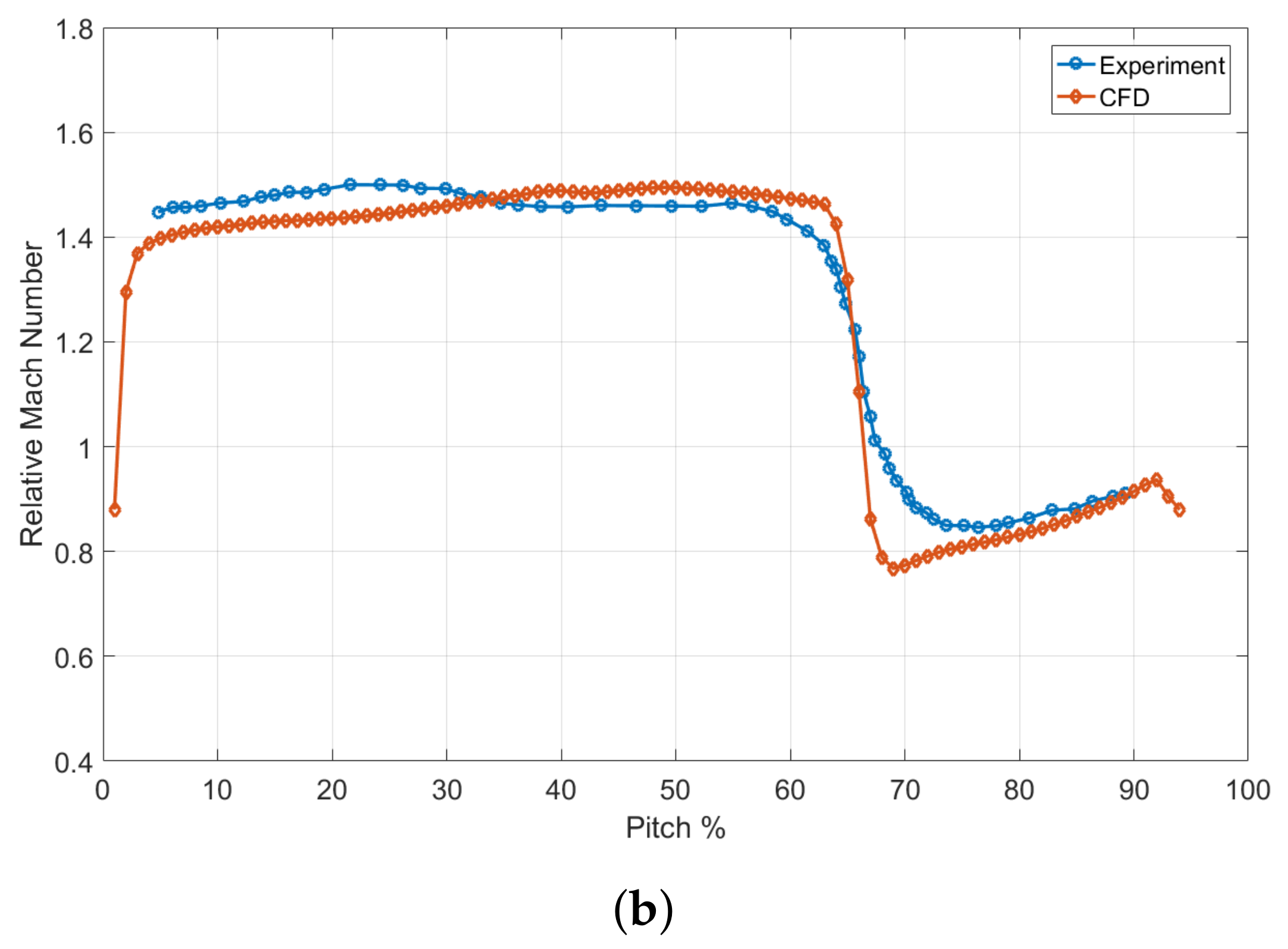
3.3. Numerical Application: NASA Rotor 37

To showcase the implementation of the baseline HBM, the first numerical application presented here regards a radial slice of the NASA rotor geometry used in Section 2.3 to validate the solver. The midspan slice of the domain was projected onto a plane to perform a 2D simulation. Being a single row domain, steady-state simulations in a relative frame of reference are usually employed for this type of configuration. Nevertheless, the study of the downstream propagation of the wake of the rotor represents an excellent spot to validate the HBM on a simple test case with a single dominant frequency (i.e., the blade passing frequency). To this purpose, the domain has been divided into three zones: the intake, the rotor and the discharge, where the first and the last are solved in the absolute frame, while the rotor is solved in a relative frame that translates with it. A linear motion with a velocity of $200 \mathrm{m}/\mathrm{s}$ in the azimuthal direction has been set for the rotor. In addition, a wake-like perturbation has been imposed at the inlet, basing on the self-similarity condition proposed by Lakshminarayana and Davino [32]. Specifically, a Gaussian perturbation with the same azimuthal wavelength as the blade pitch has been imposed in terms of total pressure and temperature:

$$\begin{array}{c}{p}_0\left(y\right)=p_{0,ref}[1-\Delta p·e^{-0.693{\left(2\frac{y}{L}\right)}^2}]\\ T_0\left(y\right)=T_{0,ref}[1-\Delta T·e^{-0.693{\left(2\frac{y}{L}\right)}^2}]\end{array}$$

where $p_{0,ref}=101325\mathrm{Pa}$ and $T_{0,ref}=288.15 \mathrm{K}$. $\Delta p$ and $\Delta T$ are the total pressure and total temperature deficits, which have been selected according to the realistic values of 0.025 and −0.007, respectively, proposed by Gomar et al. [33]. L is the wake width and has been selected as $25\%$ of the blade pitch. This non-uniform perturbation in the absolute frame is seen by the rotor as a travelling disturbance with a frequency equal to the BPF. At the same time, the rotor wake represents a travelling disturbance with the same frequency in the discharge region. We are interested in reproducing the correct behaviour of this entropy disturbances in the whole domain, as well as their interaction in the discharge region. This can be accomplished by the use of either time-resolved or HBM simulations.

Algorithm 1 Baseline HBM solution algorithm.

1: Select the base frequency $\omega$ and the number of harmonics $N_H$ 2: Set the number of snapshots $N_T\leftarrow 2N_H+1$ 3: Uniformly sample $T\leftarrow \frac{\omega }{2\pi }$ at $N_T$ instants 4: Create $N_T$ instances of the mesh of the domain 5: if Mesh is dynamic then 6:     for $i\leftarrow 0,\cdots ,N_T-1$ do 7:         Update $Mes{h}_i$ position for time $t_i$ 8:         Compute mesh flux due to $Mes{h}_i$ motion at position defined at step 7 9:     end for 10: end if 11: while Simulation not converged do 12:     Compute RHS part of the HBM source term $V\mathbf{D}{\mathcal{Q}}^n$ 13:     Initialize implicit linear system $N_T\times N_T$ block matrix $\mathit{M}$ 14:     for $j\leftarrow 0,\cdots ,N_T-1$ do 15:         Compute the flux residual ${\mathbf{R}}_{\mathbf{j}}$ and Jacobian $\frac{\partial {\mathit{R}}_{\mathit{j}}^{\mathit{n}}}{\partial {{\mathit{Q}}_{\mathit{j}}}^n}$ for $Mes{h}_j$ 16:         for $k\leftarrow 0,\cdots ,N_T-1$ do 17:            if $j==k$ then 18:                $\mathit{M}\left[j\right]\left[j\right]=\left(\frac{V}{\Delta {\tau }_j}\mathbf{I}-\frac{\partial {\mathit{R}}_{\mathit{j}}^{\mathit{n}}}{\partial {\mathit{Q}}_{\mathit{j}}^{\mathit{n}}}\right)$ 19:            else 20:                $\mathit{M}\left[j\right]\left[k\right]=V{D}_{j,k}\mathbf{I}$ 21:            end if 22:         end for 23:     end for 24:     Solve block coupled system $\mathit{M}\Delta {\mathcal{Q}}^n={\mathcal{R}}^n-V\mathbf{D}{\mathcal{Q}}^n$ 25:     ${\mathcal{Q}}^{n+1}={\mathcal{Q}}^n+\Delta {\mathcal{Q}}^n$ 26: end while

The aim is to compare the behaviour of the unsteady perturbations for three different modelling solutions: a steady-state, a time-accurate and an HBM simulation. With respect to the calculation, a second order MUSCL reconstruction with the van Leer limiter has been applied on the primitive variables for interpolation from cell centroids to face centers. The Roe scheme has been used to compute the inviscid fluxes, while a second-order centered scheme has been employed for the viscous fluxes. The $k-\omega$ SST model has been employed for turbulence closure. A pseudo Courant number of 50 has been set for the HBM, the steady-state and the inner loop of the DTS simulation. For DTS, 80 timesteps per blade passing period have been used, considering the inner loop as converged when a drop of the residuals of at least two orders of magnitude was achieved.

To compare the results for the different methods, the entropy field is calculated at the same reference relative position between the inlet wake disturbance and the blade (Figure 2). The results for the steady-state case are depicted in Figure 2a, where three blade passages are reported for the sake of clarity. In this case the interface between the different zones is treated as a “frozen rotor” Arbitrary Mesh Interface (AMI), meaning that the information is simply transferred between the two non conformal sides through a polygon-clipping conservative interpolation. It can be noticed that the wake incidence angle is discontinuous at the interfaces, both for the inlet disturbance and for the wake generated by the blade.

This non-physical effect is inherently linked to the steady-state nature of the calculation and is due to the change in the relative frame of reference at the interfaces. On the other hand, for the transient case (Figure 2d), thanks to the mesh motion, the incidence angles are correctly preserved across the interface. The HBM aims to mimic this behaviour without resorting to a transient simulation, by simply coupling a set of steady-state simulations. When a single harmonic is retained in the flow spectrum, the results are reported in Figure 2b. It can be noticed that the mere addition of a single harmonic to the mean flow is not sufficient to reconstruct the wakes shape, although they are now correctly aligned across the interfaces. In general, the thinner are the wake, the greater is the number if harmonics necessary to reconstruct their shape [33]. When three harmonics are included in the frequency set, the situation improves dramatically, as can be seen by the comparison of Figure 2c with the reference solution in Figure 2d. The inlet entropy wave and the rotor wake are correctly transferred across interfaces and their interaction in the downstream region is well captured. The entropy “bubbles” due to the poor resolution of the flow spectrum disappear, as highlighted by the close-ups in the figures. When a small number of harmonics are retained, under and overshoots can be produced, leading to non-physical values of flow quantities. This can be seen in Figure 3, where the entropy at location A (Figure 4) is plotted as a function of the pitch. The HBM solution with one harmonic is not capable of reproducing the entropy distribution across the pitch, resulting in some values falling below zero at the wake edge. On the contrary, excellent agreement is found between the three harmonics and the DTS solutions, although the former has been found to be about seven times cheaper than the latter in terms of CPU times.

4. Multi-Frequencial Harmonic Balance Method

4.1. Mathematical Formulation and Numerical Implementation

In the baseline method presented in the previous section—sometimes referred to as the time-spectral method [10]—a single fundamental frequency $\omega$ and its harmonics are present. Nevertheless, in several applications of industrial interest, multiple discrete dominant frequencies exist, which need not be integral multiples of each other. This kind of signal is defined as almost-periodic. Examples of such occurrences are multi-rows turbomachinery, in which the number of blades and vanes are typically not multiples. In such a scenario, the flow variables can still be projected into a set of arbitrary, non-harmonically related frequencies. It is important to underline that in this case the chosen frequency set does not form, in general, an orthogonal basis. Furthermore, we do not have an analytical expression for the operator $\mathbf{D}$, nor for the discrete Fourier matrix $\mathbf{E}$. Instead, the common approach is to define the matrix ${\mathbf{E}}^{-\mathbf{1}}$ analytically, and then compute numerically its inverse $\mathbf{E}$ [11,34]. In this way, the harmonic balance operator can still be defined similarly to the baseline case. Denoting with $\mathbb{F}=[{\omega }_0,{\omega }_1,\cdots ,{\omega }_K,{\omega }_{-K},\cdots ,{\omega }_{-1}]$ the vector of selected input frequencies, where ${\omega }_0=0$ and ${\omega }_{-k}=-{\omega }_k$, we can define the inverse transform matrix by its components as $E_{n,k}^{-1}=e^{i{\omega }_k{t}_n}$. Finally, the harmonic balance operator becomes simply

$$\mathbf{D}={\mathbf{E}}^{-\mathbf{1}}i\mathbf{A}\mathbf{E},\mathrm{where}{A}_{k,k}={\omega }_k$$

(23)

where $\mathbf{E}$ has been computed by numerically inverting ${\mathbf{E}}^{-\mathbf{1}}$. With this procedure, the same formulation as the baseline case can be used. Unfortunately, the presence of non-harmonically related frequencies entails that we can not always work out a fundamental period for uniform sampling of the subtime levels. Furthermore, even if a common fundamental period is present (e.g., for frequencies which are integers and coprime, see Section 4.2), we will be hardly interested in uniformly sampling that period. Indeed, this would be equivalent to a baseline HBM in which the base frequency corresponds to the common fundamental period and the discrete frequencies we are interested in are represented as harmonics of this base frequency. If the original discrete frequencies are far from each other, a huge number of harmonics needs to be considered into the spectrum (i.e., a huge number of snapshots). Therefore, we seek a way more general approach, even if the selection of sampling points typically becomes a thorny issue. Indeed, the time levels of the snapshots used during the calculation have a pivotal role in the convergence of the method. This is because the condition number of the matrix $\mathbf{E}$ is responsible for amplifying errors coming from the HB source term during the iterative solution of the equations [34].

In particular, the following conceptual differences with the baseline approach apply:

• The frequency set is composed of $N_O$ frequencies that, in general, are no longer harmonics of a common base frequency. Please notice that, in spite of this, the following relation between the minimum necessary number of samples/snapshots ($N_{T,min}$) and the number of frequencies still holds: $N_{T,min}=2N_O+1$
• Now the matrix $\mathbf{D}$ is no longer skew-symmetric. Therefore, the components on its diagonal are not zero and step 18 of Algorithm 1 must be modified according to:

  $$M\left[j\right]\left[j\right]=\left(\frac{V}{\Delta {\tau }_j}\mathbf{I}-\frac{\partial {\mathit{R}}_{\mathit{j}}^{\mathit{n}}}{\partial {\mathit{Q}}_{\mathit{j}}^{\mathit{n}}}\right)+V{D}_{j,j}\mathbf{I}$$

  (24)

It is worth noticing that for periodic flows, the Fourier matrix is always well-conditioned since the uniform sampling leads to a condition number equal to 1. This is mainly due to the orthogonality of the complex exponential basis. Conversely, when the frequency set is arbitrary, finding a set of time instants over which the matrix $\mathbf{E}$ is well conditioned is much more difficult. A variety of approaches have been proposed by several authors to overcome this issue. For example, Ekici and Hall [7] proposed an oversampling of the solution to achieve better conditioning of the matrix, while Guedeney et al. [34] used a gradient-based optimization algorithm to find a suitable set of subtime levels. In this work, we pursue the OptTP approach described by Nimmagadda et al. [17]. This approach has proved to be robust and easy to implement, and with a negligible performance drop compared to gradient-based optimization methods. The proposed method is de facto equal to the first step of the optimization method proposed by Guedeney et al. [34]. It uses a brute-force research to find the time period $T^{*}$ which minimizes the condition number of matrix $\mathbf{E}$ inside a user-defined range of possible periods, and then uniformly samples it. This operation is performed as a pre-processing step of the simulation and, due to its simplicity, it represents a negligible portion of the total CPU time. The method is detailed in Algorithm 2.

Unfortunately, this algorithm can lead to a sampling period which is much bigger than the periods corresponding to the frequencies in the set. This, in turn, could traduce in an amplification of aliasing errors in the flow spectrum. Moreover, there is no guarantee to achieve a sufficiently low value for the condition number. For these reasons, the support for oversampling was also added to our solver. The formulation in this case is exactly the same, except that now the number of time snapshots $N_T$ can be greater than $2N_O+1$. As a consequence, one must work with rectangular Fourier matrices to obtain the HB operator:

$$\underset{N_T\times N_T}{\underbrace{\mathbf{D}}}=\underset{N_T\times N_O}{\underbrace{{\mathbf{E}}^{-\mathbf{1}}}}\underset{N_O\times N_O}{\underbrace{\mathbf{A}}}\underset{N_O\times N_T}{\underbrace{{\mathbf{E}}^{+}}}$$

(25)

where ${\mathbf{E}}^{-\mathbf{1}}$ is defined as usual and ${\mathbf{E}}^{+}$ is the Moore–Penrose pseudo inverse of ${\mathbf{E}}^{-\mathbf{1}}$. Once the HB operator has been defined in this manner, no other differences exist in the solver due to oversampling, except that the code structure must allow for a different length of the snapshots vector $\mathcal{Q}$ and the frequency vector $\mathbb{F}$.

Algorithm 2 OptTP algorithm for the minimisation of the Fourier matrix condition number. As per Nimmagadda et al. [17].

1: Compute ${\omega }_{min}=min\{{\omega }_1,{\omega }_2,\cdots ,{\omega }_K\}$ and $T_0=\frac{{\omega }_{min}}{2\pi }$ 2: Form a set of test time periods $\mathbb{T}$ starting from $T_0$ and ending at $5T_0$, with a step size of $0.01T_0$ 3: Initialize $condNumber={10}^{10}$ 4: Initialize $snapshots=\underset{N_T}{\underbrace{[0,0,\cdots ,0]}}$ 5: Initialize $selectedSnapshots=\underset{N_T}{\underbrace{[0,0,\cdots ,0]}}$ 6: for $i\leftarrow 0,\cdots ,length\left(\mathbb{T}\right)-1$do 7:     Compute $T_f=\mathbb{T}\left[i\right]$ 8:     Compute $\Delta T=\frac{T_f}{N_T}$ 9:     for $k\leftarrow 0,\cdots ,N_T-1$ do 10:         $snapshots\left[k\right]=k\Delta T$ 11:     end for 12:     Calculate the inverse Fourier matrix corresponding to the time instances in $snapshots$ and the vector of frequencies $\mathbb{F}$ 13:     Calculate $thisCondNumber$ as the condition number of the inverse Fourier matrix just computed 14:     if $thisCondNumber<condNumber$ then 15:         $condNumber=thisCondNumber$ 16:         $selectedSnapshots=snapshots$ 17:     end if 18: end for

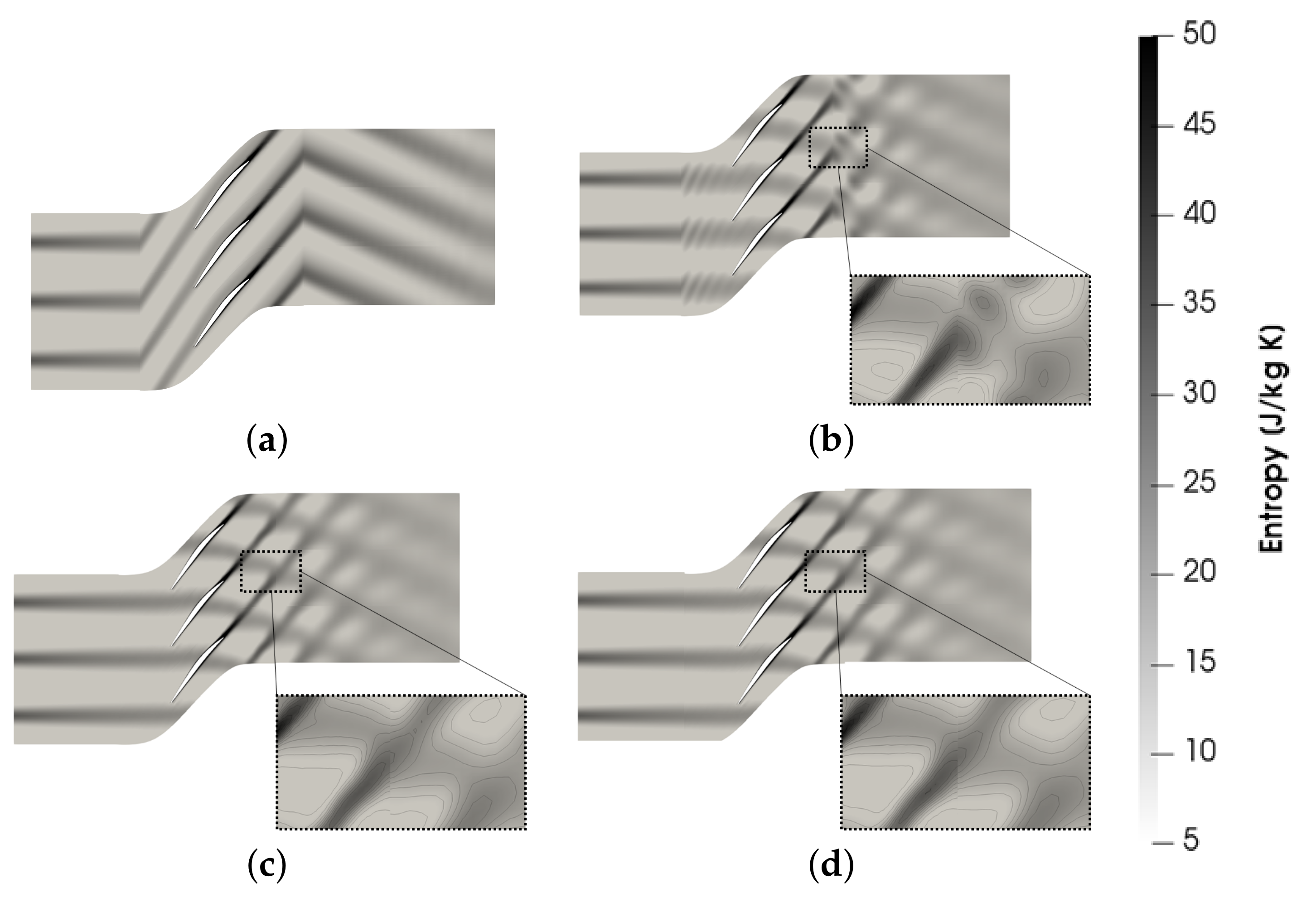
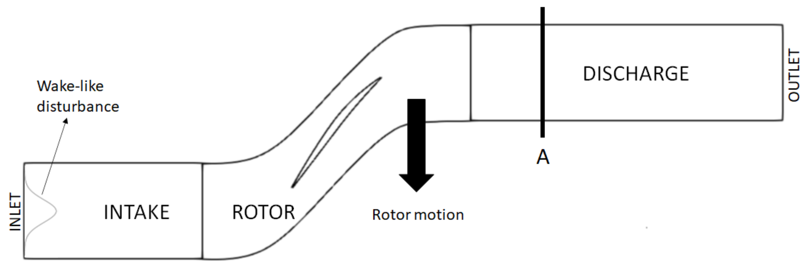
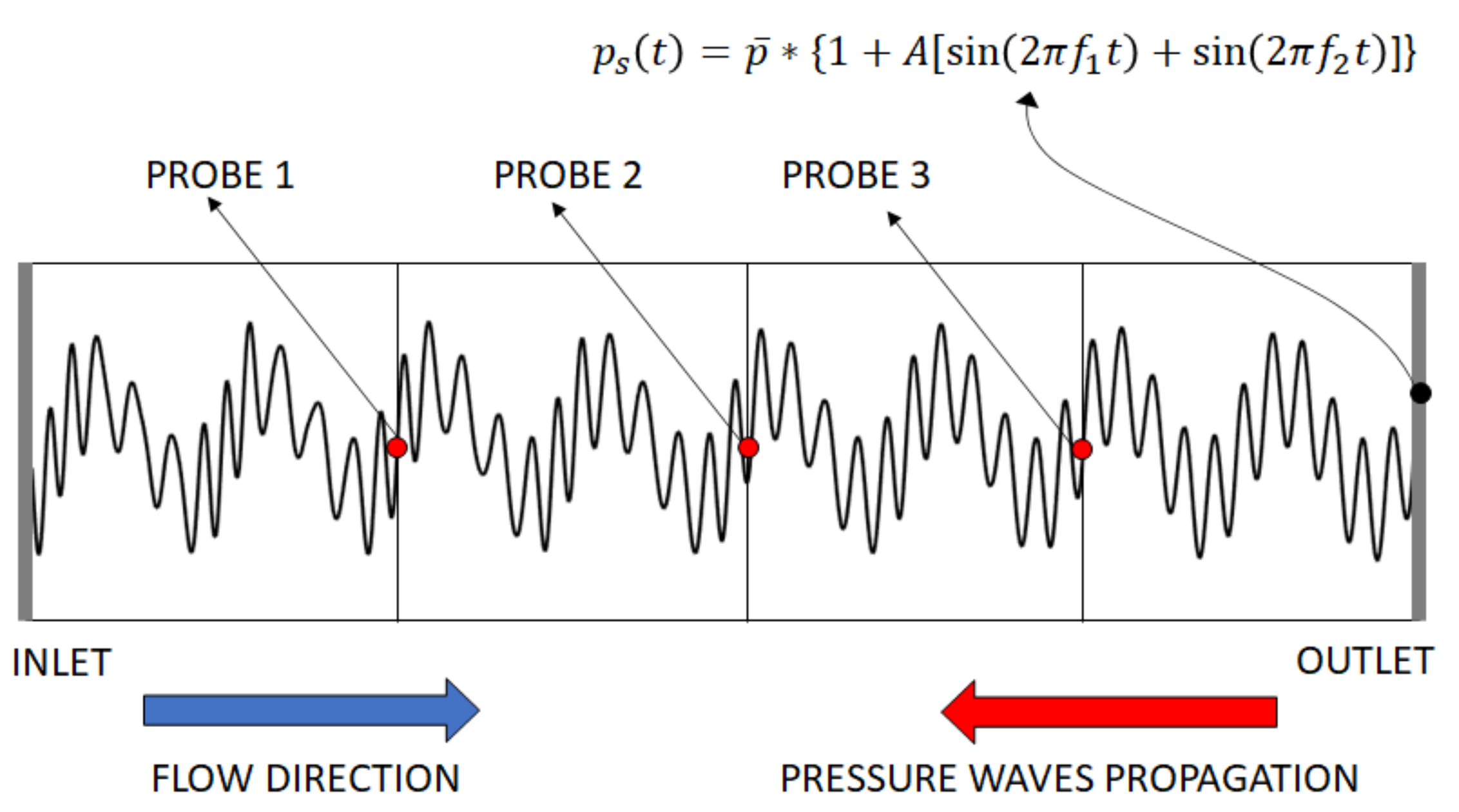
4.2. Numerical Application: Channel Flow

A test case very similar to the one used by Guedeney et al. [34] is used to validate the multi-frequential HBM implementation. It consists of a 1D channel of length $1000 \mathrm{m}$ and height $1 \mathrm{m}$ discretized with 2500 elements in the streamwise direction. At the inlet, a constant total pressure of 101,325 Pa and a total temperature of $288.15 \mathrm{K}$ are imposed. An oscillating pressure is set at the outlet

$$p_s\left(t\right)=\overline{p}·[1+A(sin2\pi f_{1}t+sin2\pi f_{2}t)]$$

(26)

where $\overline{p}$ is the $60\%$ of the inlet total pressure, $A=0.001$$f_1=3 \mathrm{Hz}$ and $f_2=17 \mathrm{Hz}$. Please notice that these two frequencies are not harmonically related but they are integer so that the flow is periodic with $T=1 \mathrm{s}$. In any case, the method is completely general and can be used for any set of harmonically and non-harmonically related frequencies. The flow is considered as inviscid and the convective fluxes are calculated by the second order Roe scheme with van Leer limiter. The time resolved simulation employs the DTS second order backward scheme with a time step of $0.001 \mathrm{s}$. A drop in the residuals of at least ${10}^{-3}$ was used for the iterative convergence in pseudo time. Twenty seconds of physical time were simulated to obtain a periodic flow.

Since the flow is subsonic throughout the channel, the objective is to observe the propagation of pressure waves from the outlet as depicted in the sketch of the domain in Figure 5. The nonlinearity of the flow triggers other frequencies in the flow spectrum as the waves propagate towards the inlet. These frequencies need to be included in the input frequency set for the HBM simulation. Strictly speaking, due to the quadratic nonlinearity of the NS equations, infinitely many frequencies are produced in the flow spectrum. These frequencies are all the linear combination of $f_1$ and $f_2$ and all their harmonics. For practical purposes, the array of solved frequencies is truncated to ${\mathbb{F}}^{*}=[f_1,2f_1,3f_1,f_2-2f_1,f_2-f_1,f_2,f_2+f_1,f_2+2f_1,f_2+3f_1]$. In this case, the algorithm described in Section 4.1 produces a condition number of the Fourier matrix equal to $1.69$. In the authors’ experience, values around $2.5$ or below can be considered satisfying for the simulation. The pressure signal is probed at three locations at $25\%$, $50\%$ and $75\%$ of the channel length, respectively, as show in Figure 5. Then the outcomes from the DTS and the HBM simulation are compared. The flow field at the desired time instants and locations for the HBM calculation can be easily reconstructed from the resultant flow spectrum through an inverse Fourier transform once the simulation has converged. The comparison is reported for each probe in Figure 6 over one period $1 \mathrm{s}$. It can be seen that the overall agreement between the two methods is good, especially for the third probe. This is to be expected, since it is the closest to the origin of pressure disturbance and therefore its spectrum is the sparser than the other two probes [34]. On the other hand, the spectrum at probe 1 location is richer and more complex, resulting in pressure peaks slightly overpredicted with respect to the DTS method. Still, the agreement is considered satisfactory throughout the channel and the method is considered validated.

4.3. Coupling between Different Zones

It is well known that in multi-stage turbomachinery, the frequencies of the unsteady flow field are linear combinations of the blade passing frequencies of the neighbouring rows [35]. For this reason, the code structure must accommodate the possibility to impose a different set of frequencies in each zone. For example, in a single stage configuration, the fundamental frequency of the HBM for either row is the passing frequency of the opposite row $\omega =N_B\mathsf{\Omega }$. The common approach to deal with single and multi-stage turbomachinery is to set different snapshots for each blade row, so that the time instants solved in each row do not necessarily match to each other. The information between adjacent zones is generated for the time levels of the receiving side through spectral interpolation of the flow field on the donor side [12], or through spatial Fourier coefficients matching [7]. The advantage of the former methods is that the coupling is performed purely in the time domain, allowing the use of non-matching radial grid lines at the interfaces. Both these techniques, however, if not properly handled through non-reflecting boundary conditions [7] or oversampling at the interface [11,12], can generate aliasing and spurious wave reflections. Furthermore, the application of non-reflecting boundary conditions to filter spurious frequencies at blade row interfaces often leads to a significant complexity in the source code. Therefore, in this work we follow another strategy, which has recently been devised by Crespo and Contreras [36] and is called the Synchronized HBM. This method bolsters the flow continuity between stator/rotor interfaces by using the same physical subtime levels all the way through the different blade rows. Since now spectral interpolation is no longer necessary at the interface, fluxes continuity is easily ensured through the use of fully conservative non-conformal interfaces. In addition, Fourier interpolation of different time instants can lead to oscillations in the solution due to the Runge phenomenon. Since in the Synchronized HBM, time instances represent a snapshot of the flow field throughout all the rows at the same time, this technique automatically refrains Runge phenomenon without the necessity to use non-reflecting boundary conditions at the interface [36]. The main drawback is that now an optimized set of instants must be retrieved to accommodate the necessity of a low condition number of the matrix $\mathbf{E}$ for all the blade rows at the same time, even for single-stage configurations. To tackle this problem, the strategy highlighted in Section 4.1 was used, and the subtime levels were selected in such a way to minimize the maximum condition number among all blade rows:

$${\mathbb{T}}^{*}=min(max\left(\kappa \left(\mathbb{T}\right)\right))$$

(27)

Following Algorithm 2, the implementation of the coupling is straightforward, since no complex non-reflecting boundary conditions or interpolation steps are necessary at blade row interfaces. It is instead sufficient to include a loop to find the maximum condition number among all rows for each test time period $\mathbb{T}$. This is the variable to minimize using Algorithm 2. Another minor drawback is that, in theory, with the non-synchronized approach, one could use a different number of snapshots in each zone (i.e., for each row) of the domain. This could speed up the calculation when it is known that the flow spectrum in some region is more sparse. Of course, this is no longer possible with the synchronized approach, where the selected number of snapshots is used throughout the whole domain.

4.4. Numerical Application: $E^3$ Axial Turbine Stage

It is now time to test the HBM on a case study of greater engineering relevance. Specifically, the midspan section of the first stage of $E^3$ engine axial turbine is studied.

The case is 2D but contains the combined complexity of coupling between different zones and the presence of different base frequencies in the flow spectrum. It must be emphasized that, as described in the previous section, if each row was sampled at its own set of time levels, the multi-frequencial approach would not be necessary. The use of the synchronized approach, on the other hand, implies that the solved time instants must be the same for the entire domain. Therefore, the columns of the Fourier matrix are not orthogonal anymore, and the multi-frequencial approach must be applied. The peculiarity is that the non-orthogonality of the basis is now caused by the selection of time instants not corresponding to the uniform sampling of any particular frequency in the spectrum, rather than the presence of multiple frequencies itself in single mesh regions.

A two vane/three blades configuration was employed in order to match the pitchwise extension of the two rows. The structured mesh was generated with ICEM CFD and is composed of 141,074 elements, selected after a grid convergence study. A turbulent viscous grid is used, ensuring a maximum $y^{+}$ value of ≈5 on the airfoil walls. The boundary conditions imposed for the simulation are reported in

Table 1. Boundary conditions for the $E^3$ axial stage simulation.

	Quantity	Value
	Total pressure	350 kPa
	Total temperature	683 K
Inlet	Turbulence intensity	3%
Outlet	Pressure	144 kPa

. Roe upwind scheme and van Leer limiter were used to achieve a second-order spacial accuracy for the convective fluxes. The central difference scheme was employed for the viscous terms. Eighty physical timesteps per blade passing were ensured for the DTS simulation, where a second-order backward scheme is employed for the temporal derivative term. A pseudo Courant number of 50 was set for the DTS as well as for the HBM simulations.

Up to five harmonics of the blade passing frequency and the vane passing frequency were retained in the spectrum of the stator and rotor regions, respectively. Interestingly, due to the particular choice of the stator/rotor blade count, the condition number obtained with the brute-force algorithm detailed in Section 4.1 was sufficiently low for all but the four harmonics case. To overcome this issue, oversampling with $3N_H+1=13$ snapshots was employed for the four harmonics simulation in order to have a small condition number of the Fourier matrix. In this way, a condition number of approximately 1 was obtained for all cases. The results for the four harmonics case are reported for the sake of completeness, although the computations is more computationally demanding than the five harmonics solution, due to the oversampling. A comparison of the entropy contours in Figure 7 reveals a good agreement between the HBM and the DTS solutions. The wakes are correctly aligned across the interface, preserving their position and their width. Remarkably, the effect of wake stretching and tilting while it is convected across the blade passages is well resolved by the HBM solution. A small difference is present in the wake of the rotor causing a slightly larger wake pattern downstream of the row. This is probably due to some self-induced vortex shedding frequencies which are not properly captured by the HBM solution. Spectral convergence is shown by means of a plot of the density and the absolute velocity magnitude as a function of the domain pitch in front of the rotor (Figure 8). Despite the complex trend across the domain pitch, the global error between the DTS and the HBM solutions gradually decreases when the spectral content of the solution is augmented. Figure 9 represents the actual amount of computational resources needed for the simulations. The plot is non-dimensionalized by the DTS simulation values, so that the values represent the CPU saving and the memory consumption factors. As expected, the latter one grows almost linearly with the number of snapshots, while the former shows a decreasing trend. It can be observed that even when 13 snapshots are used for the solution, the HBM solution is still about three times faster than the time-resolved simulation, but the memory consumption is about 19 times as much.

5. Other Relevant Issues for Turbomachinery Applications

5.1. Three-Dimensional Simulations in Cartesian Coordinates

Being a general purpose C++ library, OpenFOAM stores and computes the solution of the flow equations in cartesian coordinates. For this reason, caution should be applied when using the HBM for turbomachinery applications, in which the relevant coordinate system is the cylindrical one. This traduces in some differences in the code when applying the HB operator to a vector that rotates about the machine axis with an angular velocity equal to the revolution speed of the machine. Think for example of the time evolution of the velocity vector inside a cell of a rotating mesh during a transient turbomachinery simulation. In this case, the zeroth harmonic of the vector corresponds to a steady term in a cylindrical frame of reference rotating with the machine. On the other hand, if expressed in a cartesian reference in the absolute frame, this term represents a periodic oscillation of the velocity components with a frequency corresponding to the machine rotation frequency. In other words, the term is no longer steady if seen in the absolute frame of reference. If an HB simulation is set up with the snapshots corresponding to one or more base frequencies and their harmonics, the presence of this spurious unsteadiness will produce a non-zero component for the time derivative when it is projected on the selected frequencies through the HB operator. This is true in general even if there is only one base frequency that is a higher harmonic of the rotation frequency (e.g., the blade passing frequency and the rotation frequency), as can be easily verified numerically.

A workaround this issue is transforming the vector into a cylindrical coordinate system, then applying the HB operator and transforming the result back to the original cartesian coordinate system. In this way, the real unsteadiness is captured by the HB operator, while the spurious one related to the mesh rotation is filtered out. Finally, it is necessary to include the effect of the mesh rotation in the time derivative operator. From simple kinematic considerations, the time derivative in the absolute frame of reference of a generic vector $\mathbf{v}$ rotating with angular velocity $\mathsf{\Omega }$ can be expressed as [37]

$$\frac{\partial \mathbf{v}}{\partial t}=\mathsf{\Omega }\times \mathbf{v}$$

(28)

Please notice that this term is not required in unsteady simulations where the mesh actually undergoes a rotational displacement. On the contrary, since in our version of the HBM each dynamic mesh instance (one per snapshots) is moved in the position of the corresponding time sample and then kept fixed during the simulation, this term must be included in the momentum equation. This should not be surprising since exactly the same term ($\mathsf{\Omega }\times \rho {\mathbf{u}}_{\mathbf{k}}$) is used for MRF steady-state simulations to include the effect of the frame rotation. This term will therefore be labelled as the “steady” term. For a generic cell of the k-th snapshot’s mesh, the time derivative of the momentum can finally be expressed as

$$\frac{\partial \rho {\mathbf{u}}_{\mathbf{k}}}{\partial t}=\underset{“Steady”}{\underbrace{\mathsf{\Omega }\times \rho {\mathbf{u}}_{\mathbf{k}}}}+\underset{Unsteady}{\underbrace{\left(D_{kj}{\rho }_j{u}_j^r\right){\mathbf{e}}_{\mathbf{k}}^{\mathbf{r}}+\left(D_{kj}{\rho }_j{u}_j^{\theta }\right){\mathbf{e}}_{\mathbf{k}}^{`}+\left(D_{kj}{\rho }_j{u}_j^z\right){\mathbf{e}}_{\mathbf{k}}^{\mathbf{z}}}}$$

(29)

where ${\mathbf{u}}_{\mathbf{k}}$ is the k-th snapshot velocity vector, $u^r$, $u^{\theta }$ and $u^z$ are the radial, tangential and axial components of the velocity vector, respectively, while ${\mathbf{e}}_{\mathbf{k}}^{\mathbf{r}}$, ${\mathbf{e}}_{\mathbf{k}}^{`}$ and ${\mathbf{e}}_{\mathbf{k}}^{\mathbf{z}}$ represent the radial, tangential and axial versors, respectively. The terms inside the round brackets denote the scalar product between the k-th row of the $\mathbf{D}$ matrix and the vector containing the momentum of all the snapshots in the selected cell, following the Einstein notation on repeated indices. All this being considered, the calculation of the HB source term in the code is modified as follows:

(1)

Transform the momentum vector in cylindrical coordinates.

(2)

Apply the HB operator $\mathbf{D}$ to the momentum vector to find the time derivative approximation in cylindrical coordinates (second term on the rhs of Equation (29)).

(3)

Transform the just derived source term back to cartesian coordinates.

(4)

Add the “steady” source term as in Equation (29). This can be easily included exploiting the MRF support of the solver.

(5)

Compute the source term for the continuity and energy equation as usual, since for scalar quantities no changes are needed.

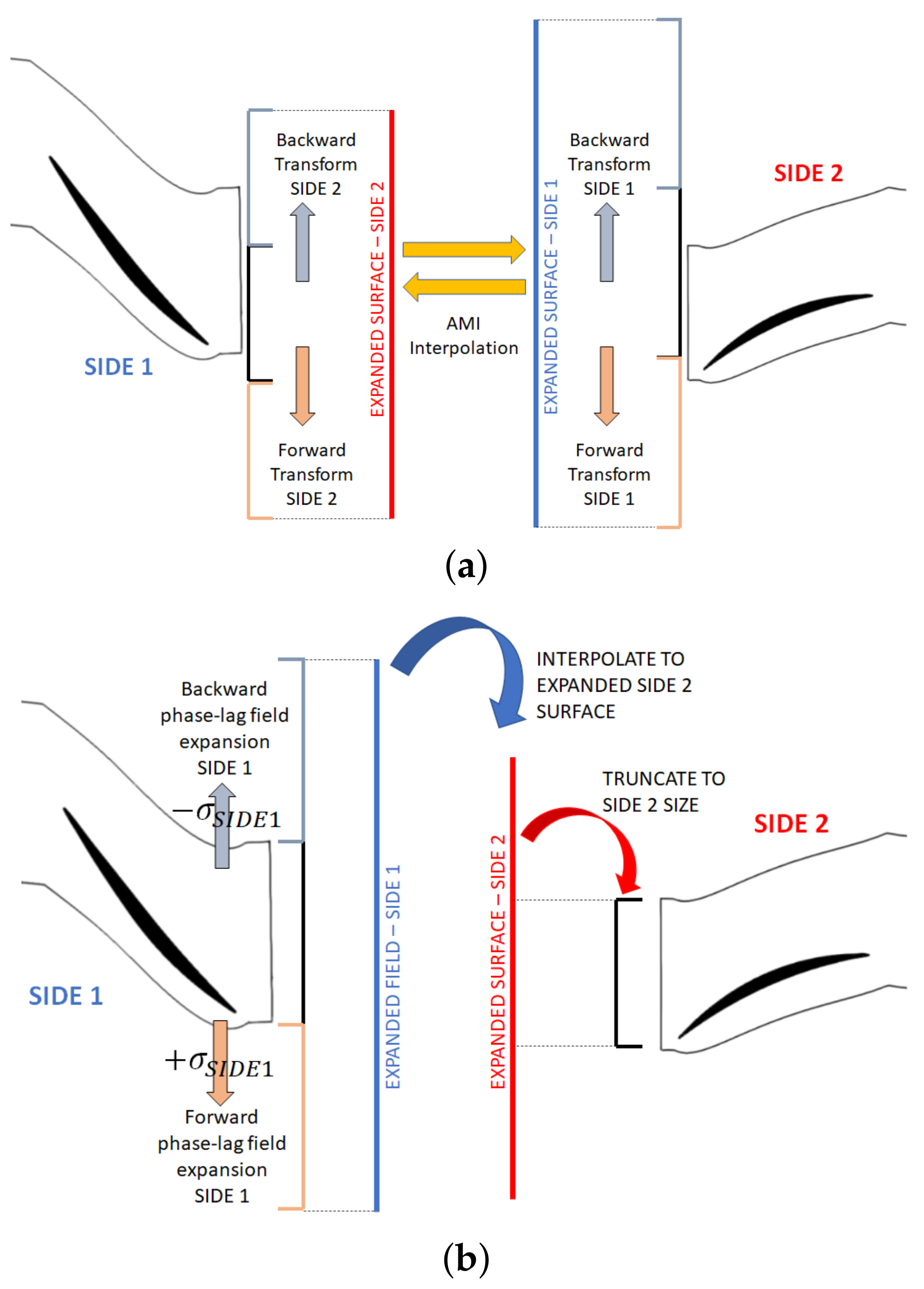
5.2. Single-Passage Reduction

Spatial periodicity in the azimuthal direction is often employed in turbomachinery simulations in order to reduce the computational domain to only a portion of the whole annulus. Nevertheless, in transient calculations, it is required to have the same pitch for the different rows, so that a large fraction of the annulus must often be simulated. This typically results in a highly increased computational effort. One technique to avoid such numerical issue is the usage of phase-lagged boundary conditions [38] and the exploitation of the chorochronic (spatio-temporal) periodicity of turbomachinery flows [39]. In this way, the computational domain can be reduced to only a single passage per blade row, independently of the blade count ratio. The method hinges upon the fact that the flow field inside a blade passage at a certain time t must be equal to the flow field in an adjacent passage at another time $t+\mathcal{T}$

$$\mathit{Q}(r,\theta +\Delta \theta ,z,t)=\mathit{Q}(r,\theta ,z,t+\mathcal{T})$$

(30)

where $\mathcal{T}$ is the time lag between the two passages, $\theta$ is the azimuthal coordinate and $\Delta \theta$ is the row pitch. Let us consider for simplicity a single-stage machine. In this case the time lag is calculated basing on the phase of a wave that travels at a rotational speed ${\omega }_k=2\pi k{f}_{BP}$ in the azimuthal direction: $\mathcal{T}=k\sigma /{\omega }_k$, where $\sigma$ is the so called interblade phase angle (IBPA). For a single stage, the IBPA in a specific row is computed basing on the relative blade count and the rotation sense [39]:

$$\sigma =-2\pi \mathrm{sgn}\left(\mathsf{\Omega }\right)\left(1-\frac{N_{B_2}}{N_{B_1}}\right)$$

(31)

where $N_{B_2}$ and $N_{B_1}$ are the number of blades in the opposite and the current blade rows, respectively. To apply phase-lagged conditions on periodic boundaries, a common approach is to update the Fourier coefficients on the boundaries at each time-step. For this reason, phase-lagged boundary conditions are very well-suited and easier to implement in frequency-domain solvers (e.g., HBM) since this kind of solver is intrinsically related to the Fourier decomposition of the solution. Indeed, an equivalent formulation of Equation (30) in the frequency domain is

$$\sum _{k=-K}^K{\widehat{\mathit{Q}}}_{\mathit{k}}(r,\theta +\Delta \theta ,z)e^{i{\omega }_{k}t}=\sum _{k=-K}^K{\widehat{\mathit{Q}}}_{\mathit{k}}(r,\theta ,z)e^{i{\omega }_{k}t}{e}^{i{\omega }_k\mathcal{T}}$$

(32)

Which entails that the flow spectrum in one passage is equal to the one of the next passage modulated by the IBPA:

$${\widehat{\mathit{Q}}}_{\mathit{k}}(r,\theta +\Delta \theta ,z)={\widehat{\mathit{Q}}}_{\mathit{k}}(r,\theta ,z)e^{i{\omega }_k\mathcal{T}}={\widehat{\mathit{Q}}}_{\mathit{k}}(r,\theta ,z)e^{ik\sigma }$$

(33)

All this being considered, and following very similar arguments as in Section 3, one can express the relation between the snapshots of the flow field on the two periodic boundaries through a linear operator as [11]

$$\mathcal{Q}(r,\theta +\Delta \theta ,z)={\mathbf{E}}^{-\mathbf{1}}\mathbf{SE}\mathcal{Q}(r,\theta ,z)$$

(34)

where $\mathbf{S}$ is a diagonal matrix whose components are $S_{kk}=e^{ik\sigma }$. The implementation of phase-lagged boundary conditions is relatively straightforward once the structure for the HBM has been built. It is sufficient to implement a new type of boundary condition which is very similar to a cyclic periodicity, here called phase-lag cyclic. The only difference is that now, when the variables are reconstructed on the faces of the periodic boundaries, Equation (34) must be used to maintain the correct phase-shift between the two sides of the coupled patches.

Now that the pitches of the various rows need not be equal to each other, the logic underpinning the exchange of information at the interface between two rows must be modified. Specifically, one needs to replicate each of the two sides of the interface an integer number of times to provide information where they do not overlap. Due to the phase-lag between the different passages, the replication needs to be carried out accordingly. Therefore, we construct a new type of interface called phase-lag Arbitrary Mesh Interface (AMI). As an example, the set up of the boundary condition is sketched in Figure 10 for a radial slice of an axial compressor stage. As can be seen from the picture, one aim of the combination of phase-lag cyclics and AMI interfaces is to obtain information about the wake from the cyclic boundaries, even if the wake is not received from the AMI interface.

The implementation follows the steps described in Algorithm 3 below and sketched in Figure 11.

Steps 1–15 are needed to calculate the weights for the interpolation on the two sides of the interface. To calculate the weights is necessary that both sides are fully paved. This is obtained by replicating the other side according to a periodic transformation (e.g., rotation by the pitch angle). These steps are performed only once as a preprocessing part of the simulation since the mesh does not change its relative position thereafter. Since the geometry replication can be performed either in the forward or the backward direction, step 8 is a way to understand if we are replicating the geometry in such a way to increase the paved area of the other side of the interface. Once we obtain as many forward and backward transformations as needed for each side, the fields can be interpolated through the interface in either direction. Therefore, during steps 16–24, the required information is exchanged from one side to the other through fields interpolation. These steps are performed once per solver iteration.

Here we presented the algorithm for a rotational geometry, but please notice that the aforementioned algorithm can be equally applied to a translational periodicity such as the $E^3$ stage presented in Section 4.4. Naturally, in this case, it is no longer necessary to transform vectors in a cylindrical frame before applying the HB and the phase-lag operators.

Algorithm 3 Phase-lag AMI algorithm.

1: Save original geometries for Side 1 and Side 2 of the interface 2: Compute weights for AMI interpolation between the two original sides 3: Initialize $NTransfForwar{d}_{Side1}=0$ and $NTransfBackwar{d}_{Side1}=0$ 4: while Side 2 of the interface is not fully paved do 5:     Replicate the original geometry of Side 1 of the interface according to the periodic transformation (e.g., rotate by pitch periodicity angle, Figure 11a) 6:     Append the transformed geometry to Side 1 of the interface 7:     Recalculate weights for AMI interpolation between the two sides 8:     if the sum of the new weights is lower than the previous one then reverse the direction of the transformation in step 4 9:     end if 10:     if We are transforming in the forward direction then    $NTransfForwar{d}_{Side1}++$ 11:     else   $NTransfBackwar{d}_{Side1}++$ 12:     end if 13: end while 14: Repeat steps 3–13 for the other side of the interface 15: Compute the AMI weights for the two expanded sides of the interface (Figure 11a) 16: ... 17: for $i\leftarrow 0,\cdots ,NTransfForwar{d}_{Side1}-1$do 18:     Expand the field on Side 1 of the interface according to the phase-lag boundary conditions (34) with a positive IBPA (Figure 11b) 19: end for 20: for $i\leftarrow 0,\cdots ,NTransfbackwar{d}_{Side1}-1$do 21:     Expand the field on Side 1 of the interface according to the phase-lag boundary conditions (34) with a negative IBPA (Figure 11b) 22: end for 23: Interpolate the expanded field on Side 1 of the interface onto the expanded surface of Side 2 thanks to the AMI weights previously calculated (Figure 11b). 24: Truncate the interpolated field to the size of the Side 2 of the interface to obtain the required information (Figure 11b). 25: Repeat steps 17–23 for the other side of the interface.

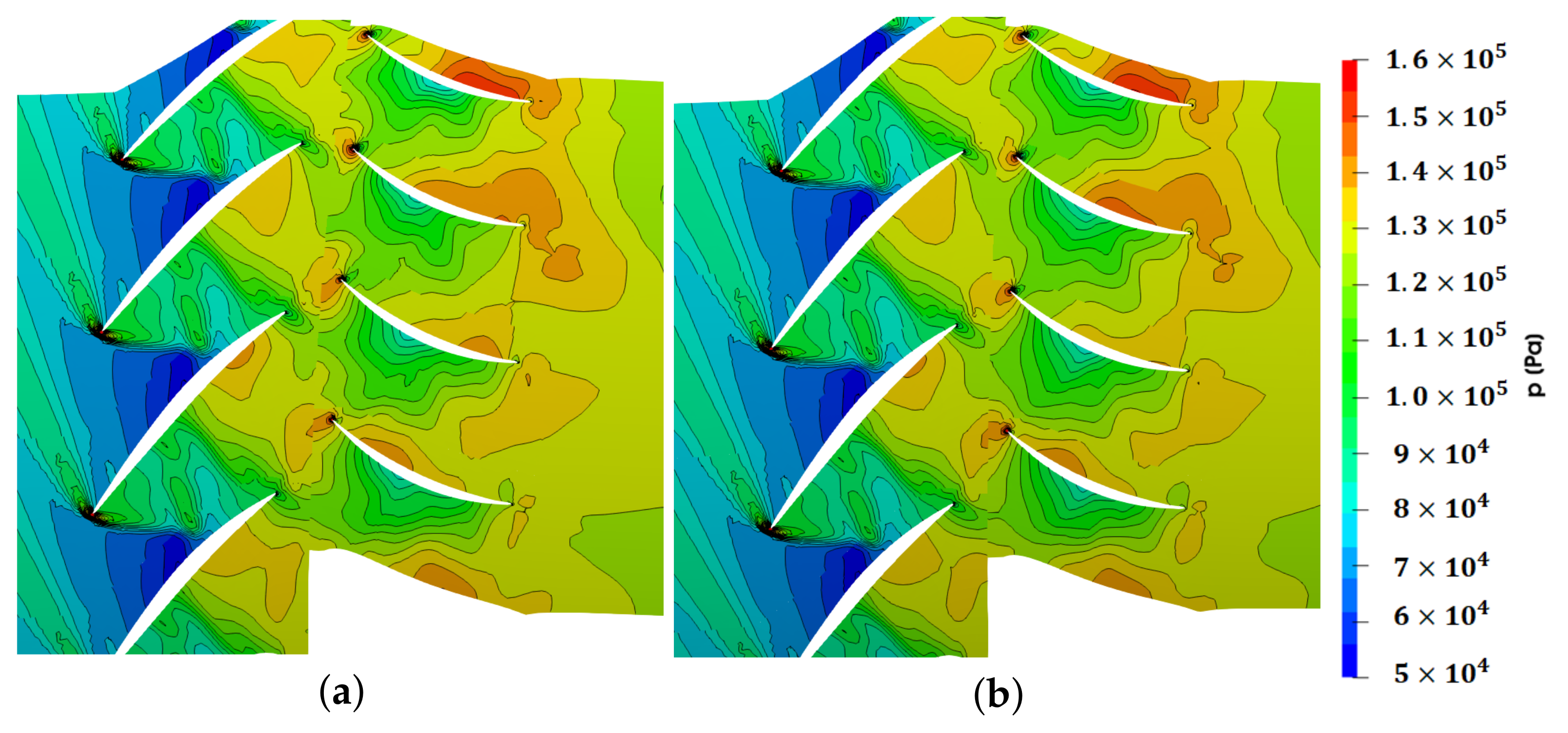
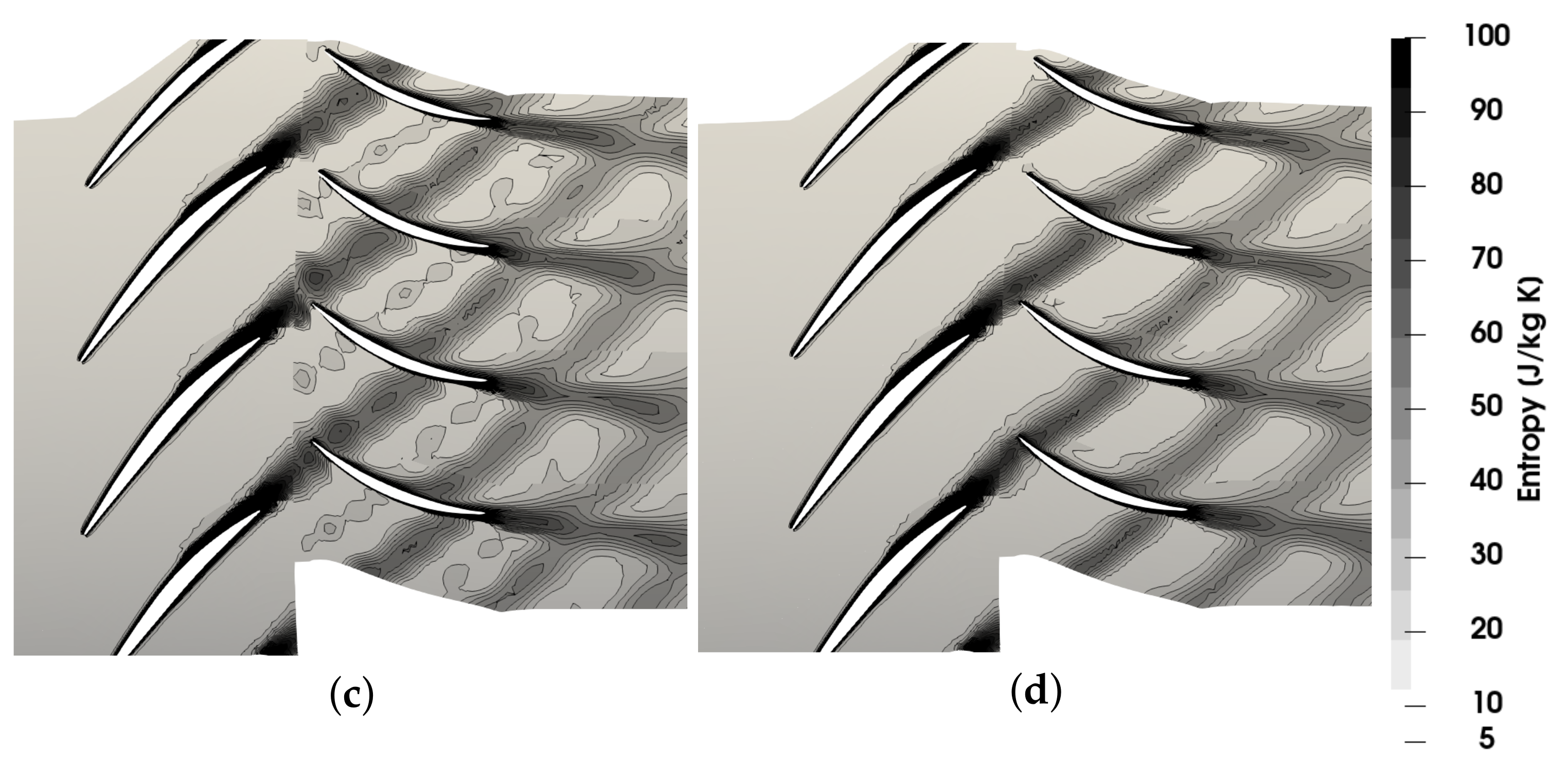
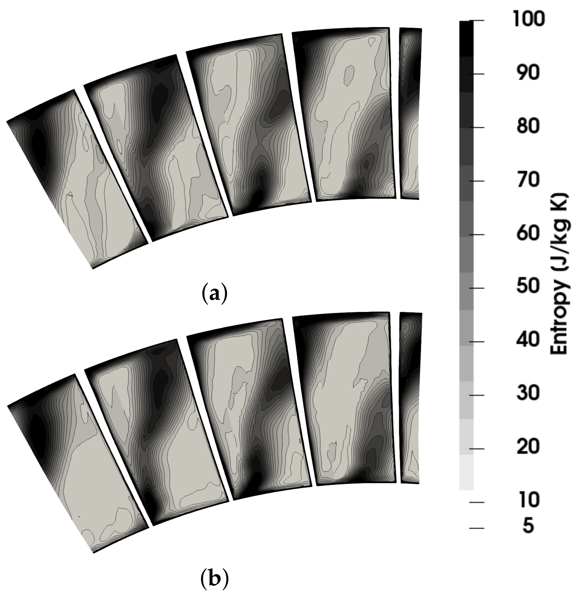
5.3. Numerical Application: NASA Stage 37

The last application presented aims to include all the building blocks of the HBM that were illustrated in the previous sections. The 3D geometry of the NASA stage 37 [28] is selected for such purpose. The geometry consists of 36 blades rotating at 18,000 rpm and 46 vanes. Only one blade passage per row is modelled according to the single passage reduction method illustrated in Section 5.2. Up to four harmonics of the passing frequencies of each row have been considered in the spectrum. Once again, the Roe upwind scheme was employed for the convective fluxes, in combination to a second-order MUSCL reconstruction with van Leer limiter. A pseudo Courant number of 25 was used for the local time stepping integration. Since the mesh does not change topology from one snapshot to another, the code parallelization has been carried out in a simple and efficient way. The domain decomposition is performed only on the original mesh, and maintained for all the snapshots. In this way, corresponding cells from different snapshots are kept on the same processor. Since the calculation of the HBM source term does not require the values of the conservative variables in adjacent cells, no communication between processors is necessary during the computation of this term.

For the calculation with four harmonics of the blade passing frequency, the HBM required approximately 600 core-hours. Please notice that a comparable time-resolved simulation would require modelling half the annulus (18 blades and 23 vanes), which is approximately twenty times the size of the current simulation. Assuming to use 80 physical time steps per blade passing and 20 subiterations for the inner loops, at least 2/3 complete revolutions of the rotor are usually necessary to reach a periodic behaviour. This results in an estimated simulation time about two orders of magnitude larger than the HBM, depending on the number of frequencies included in the spectrum. No oversampling was necessary in this case, since the maximum condition number was obtained for the simulation with four harmonics and was equal to $1.77$.

Figure 12illustrates the results for the simulations with two and four harmonics of the passing frequencies in terms of instantaneous pressure and entropy contours in a midspan section of the annulus. The flow field has been reconstructed at the desired time and four adjacent passages are reported taking into account the phase-lag between them. It can be noticed that the wakes are resolved with a better resolution across the interface and in the downstream blade row for the four harmonics simulation, as well as the pressure disturbances due to the bow waves interaction with the upstream row. Overall, an improved resolution of the periodic disturbance is obtained across the compressor span, as depicted in Figure 13, where the entropy contours on an axial plane cutting the vane at $20\%$ of the chord are shown. As observed in the previous sections, the use of a higher number of harmonics leads to a better localization in time and space of the disturbances, thanks to a lower degree of under/overshoots in the flow quantities. As a final comparison, the time evolution of the total forces over one passing period has been reported for the rotor and the stator in Figure 14. It can be observed that, by increasing the number of harmonics, the solution tends to converge to a fixed distribution over the time period. Please notice that conventional steady-state methods (e.g., mixing plane) would predict a constant value over time which is not necessary close to the time-averaged value resulting from a time-resolved simulation.

6. Conclusions

This work has illustrated how a fully implicit HBM can be implemented step-by-step in a CFD code. The choice has fallen upon the open-source software OpenFOAM, due to its wide diffusion and high-standard C++ compliance, trying to propose an implementation as far-reaching as possible. First of all, a new density-based solver is presented and validated in the OF framework, forming the basis for the HB support. The paper then proceeds on a combined theoretical and practical approach, starting from the fully-implicit baseline HBM and progressively adding other important features such as multi-frequencial support and phase-lagged boundary conditions. A research algorithm combined with a synchronized approach are used to improve flow continuity at the interfaces. This also allows to minimize the propagation of errors in the solution that possibly arises from a bad conditioning of the Fourier matrix. Four test cases have been proposed to verify the correct implementation of the different features. For the baseline HBM, disturbances propagation in a multi-region domain has been studied, showing the differences between the steady-state and the HB methods. It is shown that retaining three harmonics of the blade passing frequency in the spectrum is sufficient to reproduce the transient solution with a negligible error. The multi-frequencial approach has been tested at first on a simplified channel flow and then has been applied to a real axial turbine stage. Both test cases have shown a satisfactory agreement with the reference unsteady solutions. For the axial turbine case, it is reported that five harmonics of the passing frequency are adequate to capture transient effects. Finally, the addition of phase-lag boundary conditions on periodic boundaries and blade-row interfaces has been illustrated for an axial compressor stage. It is also shown that the correct formulation of the HB operator in cartesian coordinates allows to produce the correct solution for rotationally periodic geometries. Conclusions are also drawn with respect to the performance of the HB solver compared to time-resolved simulations. Specifically, the CPU saving factor strongly depends on the specific application and the number of frequencies considered in the spectrum. Broadly speaking, in case of identical domains for time-resolved and HBM solutions, a reduction in the CPU time of an order of magnitude can be expected, as well as an increase of one order of magnitude in the memory consumption. For turbomachinery cases where the domain is reduced to a single passage per row through phase-lagged boundary conditions, a reduction in CPU time of nearly two order of magnitude can be easily achieved.

References

1. Tucker, P. Computation of unsteady turbomachinery flows: Part 1—Progress and challenges. Prog. Aerosp. Sci. 2011, 47, 522–545. [Google Scholar] [CrossRef]
2. Tucker, P. Computation of unsteady turbomachinery flows: Part 2—LES and hybrids. Prog. Aerosp. Sci. 2011, 47, 546–569. [Google Scholar] [CrossRef]
3. Berkooz, G.; Holmes, P.; Lumley, J. The Proper Orthogonal Decomposition in the Analysis of Turbulent Flows. Annu. Rev. Fluid Mech. 2003, 25, 539–575. [Google Scholar] [CrossRef]
4. He, L.; Ning, W. Efficient Approach for Analysis of Unsteady Viscous Flows in Turbomachines. AIAA J. 1998, 36, 2005–2012. [Google Scholar] [CrossRef]
5. Hall, K.C.; Thomas, J.P.; Clark, W.S. Computation of Unsteady Nonlinear Flows in Cascades Using a Harmonic Balance Technique. AIAA J. 2002, 40, 879–886. [Google Scholar] [CrossRef] [Green Version]
6. Ekici, K.; Hall, K.C. Harmonic Balance Analysis of Limit Cycle Oscillations in Turbomachinery. AIAA J. 2011, 49, 1478–1487. [Google Scholar] [CrossRef]
7. Ekici, K.; Hall, K.C. Nonlinear Analysis of Unsteady Flows in Multistage Turbomachines Using Harmonic Balance. AIAA J. 2007, 45, 1047–1057. [Google Scholar] [CrossRef]
8. Thomas, J.P.; Dowell, E.H.; Hall, K.C. Nonlinear Inviscid Aerodynamic Effects on Transonic Divergence, Flutter, and Limit-Cycle Oscillations. AIAA J. 2002, 40, 638–646. [Google Scholar] [CrossRef]
9. Jameson, A.; Alonso, J.; McMullen, M. Application of a non-linear frequency domain solver to the Euler and Navier-Stokes equations. In Proceedings of the 40th AIAA Aerospace Sciences Meeting & Exhibit, Reno, NV, USA, 14–17 January 2002. [Google Scholar]
10. Van der Weide, E.; Gopinath, A.; Jameson, A. Turbomachinery Applications with the Time Spectral Method. In Proceedings of the 35th AIAA Fluid Dynamics Conference and Exhibit, Toronto, ON, Canada, 6–9 June 2005; p. 4905. [Google Scholar]
11. Gopinath, A.; van der Weide, E.; Alonso, J.; Jameson, A.; Ekici, K.; Hall, K. Three-Dimensional Unsteady Multi-stage Turbomachinery Simulations Using the Harmonic Balance Technique. In Proceedings of the 45th AIAA Aerospace Sciences Meeting and Exhibit, Reno, NV, USA, 14–17 January 2007. [Google Scholar]
12. Sicot, F.; Dufour, G.; Gourdain, N. A time-domain harmonic balance method for rotor/stator interactions. J. Turbomach. 2012, 134. [Google Scholar] [CrossRef] [Green Version]
13. Su, X.; Yuan, X. Implicit solution of time spectral method for periodic unsteady flows. Int. J. Numer. Methods Fluids 2010, 63, 860–876. [Google Scholar] [CrossRef]
14. Woodgate, M.A.; Badcock, K.J. Implicit Harmonic Balance Solver for Transonic Flow with Forced Motions. AIAA J. 2009, 47, 893–901. [Google Scholar] [CrossRef]
15. Sicot, F.; Puigt, G.; Montagnac, M. Block-Jacobi Implicit Algorithms for the Time Spectral Method. AIAA J. 2008, 46, 3080–3089. [Google Scholar] [CrossRef]
16. Thomas, J.P.; Custer, C.H.; Dowell, E.H.; Hall, K.C.; Corre, C. Compact Implementation Strategy for a Harmonic Balance Method Within Implicit Flow Solvers. AIAA J. 2013, 51, 1374–1381. [Google Scholar] [CrossRef]
17. Nimmagadda, S.; Economon, T.D.; Alonso, J.J.; da Silva, C.R.I. Robust uniform time sampling approach for the harmonic balance method. In Proceedings of the 46th AIAA Fluid Dynamics Conference, Washington, DC, USA, 13–17 June 2016. [Google Scholar]
18. Cvijetić, G.; Gatin, I.; Vukčević, V.; Jasak, H. Harmonic Balance developments in OpenFOAM. Comput. Fluids 2018, 172, 632–643. [Google Scholar] [CrossRef]
19. Oliani, S.; Casari, N.; Pinelli, M.; Suman, A.; Carnevale, M. Numerical study of a centrifugal pump using Harmonic Balance Method in OpenFOAM. In Proceedings of the 34th International Conference on Efficiency, Cost, Optimization, Simulation and Environmental Impact of Energy Systems, Taormina, Italy, 28 June–2 July 2021. [Google Scholar]
20. Hall, K.C.; Ekici, K.; Thomas, J.P.; Dowell, E.H. Harmonic balance methods applied to computational fluid dynamics problems. Int. J. Comput. Fluid Dyn. 2013, 27, 52–67. [Google Scholar] [CrossRef]
21. He, L. Fourier methods for turbomachinery applications. Prog. Aerosp. Sci. 2010, 46, 329–341. [Google Scholar] [CrossRef]
22. Luo, H.; Baum, J.D.; Löhner, R. A Fast, Matrix-free Implicit Method for Compressible Flows on Unstructured Grids. J. Comput. Phys. 1998, 146, 664–690. [Google Scholar] [CrossRef] [Green Version]
23. Blazek, J. Computational Fluid Dynamics: Principles and Applications, 3rd ed.; Butterworth-Heinemann: Woburn, MA, USA, 2015. [Google Scholar]
24. Saad, Y.; Schultz, M.H. GMRES: A generalized minimal residual algorithm for solving nonsymmetric linear systems. Siam J. Sci. Stat. Comput. 1986, 7, 856–869. [Google Scholar] [CrossRef] [Green Version]
25. Yoon, S.; Jameson, A. Lower-upper Symmetric-Gauss-Seidel method for the Euler and Navier-Stokes equations. AIAA J. 1988, 26, 1025–1026. [Google Scholar] [CrossRef] [Green Version]
26. Heyns, J.; Oxtoby, O. Modelling high-speed viscous flow in OpenFOAM®. In Proceedings of the 9th South African Conference on Computational and Applied Mechanics, Somerset West, South Africa, 14–16 January 2014. [Google Scholar]
27. Dunham, J. CFD Validation for Propulsion System Components; Technical Report AR-355; AGARD: Neuilly-sur-Seine, France, 1998. [Google Scholar]
28. Reid, L.; Moore, R.D. Design and Overall Performance of Four Highly Loaded, High Speed Inlet Stages for an Advanced High-Pressure-Ratio Core Compressor; Technical Report 1337; NASA: Washington, DC, USA, 1978.
29. Suder, K.L. Experimental Investigation of the Flow Field in a Transonic, Axial Flow Compressor with Respect to the Development of Blockage and Loss; Technical Report 107310; NASA: Washington, DC, USA, 1996.
30. McMullen, M.S.; Jameson, A.; Alonso, J.J. Demonstration of Nonlinear Frequency Domain Methods. AIAA J. 2006, 44, 1428–1435. [Google Scholar] [CrossRef] [Green Version]
31. Frey, C.; Ashcroft, G.; Kersken, H. Simulations of Unsteady Blade Row Interactions Using Linear and Non-Linear Frequency Domain Methods. In Proceedings of the ASME Turbo Expo 2015: Turbomachinery Technical Conference and Exposition, Montreal, QC, Canada, 15–19 January 2015. [Google Scholar]
32. Lakshminarayana, B.; Davino, R. Mean Velocity and Decay Characteristics of the Guidevane and Stator Blade Wake of an Axial Flow Compressor. J. Eng. Power 1980, 102, 50–60. [Google Scholar] [CrossRef]
33. Gomar, A.; Bouvy, Q.; Sicot, F.; Dufour, G.; Cinnella, P.; François, B. Convergence of Fourier-based time methods for turbomachinery wake passing problems. J. Comput. Phys. 2014, 278, 229–256. [Google Scholar] [CrossRef] [Green Version]
34. Guédeney, T.; Gomar, A.; Gallard, F.; Sicot, F.; Dufour, G.; Puigt, G. Non-uniform time sampling for multiple-frequency harmonic balance computations. J. Comput. Phys. 2013, 236, 317–345. [Google Scholar] [CrossRef] [Green Version]
35. Tyler, J.M.; Sofrin, T.G. Axial Flow Compressor Noise Studies; SAE Technical Paper; SAE International: Warrendale, PA, USA, 1962. [Google Scholar]
36. Crespo, J.; Contreras, J. On the Development of a Synchronized Harmonic Balance Method for Multiple Frequencies and its Application to LPT Flows. In Proceedings of the ASME Turbo Expo 2020: Turbomachinery Technical Conference and Exposition, London, UK, 22–26 June 2020. [Google Scholar]
37. Greitzer, E.M.; Tan, C.S.; Graf, M.B. Internal Flow: Concepts and Applications; Cambridge Engine Technology Series; Cambridge University Press: New York, NY, USA, 2004. [Google Scholar]
38. Erdos, J.I.; Alzner, E.; McNally, W. Numerical Solution of Periodic Transonic Flow through a Fan Stage. AIAA J. 1977, 15, 1559–1568. [Google Scholar] [CrossRef]
39. Gerolymos, G.A.; Michon, G.J.; Neubauer, J. Analysis and Application of Chorochronic Periodicity in Turbomachinery Rotor/Stator Interaction Computations. J. Propuls. Power 2002, 18, 1139–1152. [Google Scholar] [CrossRef]
Figure 1. Numerical code validation against experimental results from [29]. (a) Relative Mach number contours at 70 % span obtained with the CFD code (left) and experimentally (right). (b) Relative Mach number along the pitch at 70 % span and 20 % chord for the near peak efficiency condition.
Machines 10 00279 g001aMachines 10 00279 g001b
Figure 2. Entropy field obtained with the three different methods and different number of harmonics included in the flow spectrum. (a) Steady-state frozen rotor; (b) 1 Harmonic; (c) 3 Harmonics; (d) DTS.
Machines 10 00279 g002
Figure 3. Entropy profile in the wake at plane A for HBM and DTS.
Machines 10 00279 g003
Figure 4. Domain of the NASA rotor 37 test case for the baseline HBM.
Machines 10 00279 g004
Figure 5. Domain and boundary conditions for the channel flow test case.
Machines 10 00279 g005
Figure 6. Comparison between HBM and DTS for the pressure signal registered by the three probes for the channel flow test case. (a) Probe 1. (b) Probe 2. (c) Probe 3.
Machines 10 00279 g006
Figure 7. Comparison of entropy contours for the E 3 axial turbine stage test case. (a) Five harmonics. (b) DTS.
Machines 10 00279 g007
Figure 8. Instantaneous flow quantities in front of the rotor blades as a function of the blade pitch for the DTS and HBM simulations. (a) Density. (b) Absolute velocity magnitude.
Machines 10 00279 g008
Figure 9. Comparison of the CPU factors required for the HBM and the DTS calculations. The plot is non-dimensionalised by the DTS simulation values.
Machines 10 00279 g009
Figure 10. Illustration of the phase-lagged boundary condition behaviour.
Machines 10 00279 g010
Figure 11. Illustration of Algorithm 3 for the implementation of phase-lag AMI interfaces. (a) Steps 1–16. (b) Steps 17–25.
Machines 10 00279 g011
Figure 12. Contours on a radial slice at midspan for the NASA stage 37 test case. (a) Pressure contours for 2 harmonics. (b) Pressure contours for 4 harmonics. (c) Entropy contours for 2 harmonics. (d) Entropy contours for 4 harmonics.
Machines 10 00279 g012aMachines 10 00279 g012b
Figure 13. Entropy contours on an axial plane at 20% of the vane chord. (a) Two harmonics. (b) Four harmonics.
Machines 10 00279 g013
Figure 14. Evolution of forces on stator and rotor blades over one passing period. (a) Rotor. (b) Stator.
Machines 10 00279 g014