Progressive Improvement of the Model of an Exoskeleton for the Lower Limb by Applying the Modular Modelling Methodology

Abstract

Among the variety of applications of exoskeletons, it is possible to mention motor rehabilitation, enhancement of human capabilities and providing support to different types of tasks. Despite the remarkable achievements in this field, two major issues still need to be improved in the exoskeleton design methodology, the mechanical design and the controller. Considering that the dynamic modelling approach plays a key role in these issues, this article proposes the use of modular modelling methodology for the development of exoskeletons. Initially, the conceptual design of a lower limb exoskeleton is presented, then its kinematic and dynamic models are calculated. Finally, some performed simulations demonstrate the model consistency and the actuator torques estimation.

1. Introduction

In mechatronics engineering, an exoskeleton can be defined as a wearable robot that acts as a robotic orthosis on the user [1]. Exoskeletons have different applications, namely, motor rehabilitation, enhancement of human capabilities and providing support to different types of tasks, ranging from work to daily life activities. They can be designed to be used by healthy subjects in order to augment their capabilities, e.g., carry large weights, or for people with disabilities that may rely on the exoskeleton to be able to perform simple tasks such as taking a glass of water.

These variety of applications have something in common: the exoskeleton is acting in parallel with the human body, hence, it should reproduce human movements at a functional level [2]. This requires the design of robotic systems with a large number of degrees of freedom (dof), for instance, up to seven dofs for the upper limb without considering the hand [3] and up to twelve dofs for the lower limb [4]. Therefore, this imposes some requirements on the mechanical design. Moreover, the exoskeleton must be designed to intervene in a certain way and interact with the movement of the user [5]. In order to do so, it is important to control the interaction force between the user and robot using, for instance, impedance control [6].

In the nineteen-sixties, the first powered exoskeleton, Hardiman, was developed. Later, in the nineteen-nineties, the military prototype from the University of Berkeley, called BLEEX, was presented [7]. The assistive robots must be able to amplify the residual movements of a patient suffering from muscle weakness or neurological diseases. In such case, next to the mechanical design challenges, as the exoskeleton has to adapt to the deformities of the patients, it needs to identify their intentions in order to provide the correct assistance. In this respect, the HAL-5 from Cyberdyne Inc., (Japan) was designed to help the elderly and handicapped people to walk. The intention of the user is measured by EMG, which is then used to control electrical motors [8].

Kazerooni and Steger [9] continued the development of BLEEX. They modelled it attached to human legs, only in the sagittal plane, and derived the inverse dynamics model for predicting the driving torques during the walking cycle phases. Additionally, they focused on the 1-dof feedback controller and its implementation. Acosta-Marquez and Bradley [10] presented a simple and lightweight exoskeleton for mobility in constrained environments, which employed crutches. They also developed a controller in order to satisfy some energy requirements.

Regarding the dynamic modelling, the Newton–Euler approach and the principle of virtual work are classical formalisms for generating the equations in implicit form [11]. Moreover, the computational efficiency can be greatly enhanced by the use of recursive algorithms [12]. On the other hand, the Lagrangian formulation is more suitable for obtaining those equations in explicit form. However, such an approach becomes prohibitive when dealing with closed-loop mechanisms [13]. In particular, with respect to the development of exoskeletons, there is an additional demand related to the easiness in building the dynamic model and modifying it as well.

Anam and Al-Jumaily [14] classified the control approaches for powered exoskeletons into four categories, namely, model-based, hierarchy-based, physical-parameter-based and usage-based controls. With respect to the model-based control, there are the mathematical model, the identification model, the AI model and the muscle model. Regarding the hierarchy-based control, there are three levels: the task, the high and the low levels. For the physical-parameter-based control, at the low level, there are the PID, the sliding mode, the LQ and H${}_{\infty }$, while at the high level (interaction between the exoskeleton with the human being), impedance and admittance control are employed. With respect to the usage-based control, one can mention the virtual reality, teleoperation and gait pattern. Regarding this trend, one can mention the importance of developing exoskeletons that combine the three levels, detect user intention, have intrinsic modularity and use the distributed but not centralised control approach.

Concerning the unpowered exoskeletons, Agrawal et al. [15] developed a gravity-balanced mechanism by using tension springs. They developed the inverse dynamics model by applying the Newton–Euler approach. After performing several experimental tests, they noticed an increase of the range of motion for both the hip and knee. Collins et al. [16] developed an exoskeleton for the ankle that consisted of a mechanical clutch and a spring. From the analysis of the obtained results, they concluded that it was more energy-effective at walking.

Therefore, those considerations raise two major problems in the exoskeleton design, the mechanical design and the controller. The mechanical design also needs to have some flexibility in order to allow the adaptation of actions to different groups of people. Moreover, the model of the controller needs an accurate representation of the mechanical system. Therefore, the mechanical modelling technique should be capable of changing the parameters to adjust to users with different sizes and requirements. This is particularly important for a lower limb exoskeleton during its adaptation to the legs of the user. In order to do so, there is room for improvement in the mechanical modelling procedures currently available.

This article proposes a dynamic modelling approach based on the modular modelling methodology (MMM) for the progressive improvement of exoskeletons. The conceptual design of a lower limb exoskeleton is described in Section 2. In Section 3, the theoretical background related to the Gibbs–Appell and modular dynamic modelling methods is presented. In Section 4, its kinematic and dynamic models are carried out. Then, Section 5 shows the performed simulations and obtained results. Finally, in Section 6, the conclusions are drawn.

2. The Modular Modelling Methodology

Among the possible forms of deriving the equations of motion, one is that expressed by Equation (1) [17,18] which is known as either Gibbs–Appell’s or Kane’s approach. Hence, the dynamic model of a N-body mechanical system can be obtained from the sum of dot products between the partial velocities and active/inertial efforts.

$$\sum _{k=1}^N\frac{\partial {\mathbf{v}}_{G_k}^T}{\partial \dot{q_i}}\left({\mathbf{F}}_{a_k}-m_k{\dot{\mathbf{v}}}_{G_k}\right)+\frac{\partial {\mathit{\omega }}_k^T}{\partial \dot{q_i}}\left({\mathbf{M}}_{a_k}-({\left[I\right]}_k{\dot{\mathit{\omega }}}_k+{\mathit{\omega }}_k\times {\left[I\right]}_k{\mathit{\omega }}_k)\right)=\mathbf{0}$$

(1)

$$i=1,\dots ,\mu$$

Alternatively, in order to systematise the derivation of the dynamic equations, Orsino and Hess-Coelho [19,20,21] proposed another representation for Gibbs–Appell’s or Kane’s method. Basically, it comprises the utilisation of redundant variables and coupling matrices for defining the variable dependency with the generalised velocities. Hence, the inclusion of bodies, subsystems and dynamic effects becomes relatively easier. It is called the modular modelling methodology [22]. For a system S with $\mu$ degrees of freedom, ${\dot{q}}_1,{\dot{q}}_2,\dots ,{\dot{q}}_{\mu }$ are the generalized velocities and the kinematic variables of the kth body can be defined as

$${\left[\begin{array}{c}{}^0{\mathbf{v}}_G\\ {}^k\mathit{\omega }\end{array}\right]}_k=\left[\begin{array}{c}{u}_1\\ ⋮\\ u_{{\lambda }_k}\end{array}\right]=C_k\left[\begin{array}{c}{\dot{q}}_1\\ ⋮\\ {\dot{q}}_{\mu }\end{array}\right]$$

(2)

where ${\lambda }_k$ is the dimension of vector ${\left[{}^0{\mathbf{v}}_G{}^k\mathit{\omega }\right]}^T$ (3 for planar and 6 for spatial motions) and the coupling matrix $C_k$ is

$$C_k={\left[\begin{array}{ccc}\frac{\partial u_1}{\partial {\dot{q}}_1}& \dots & \frac{\partial u_1}{\partial {\dot{q}}_{\mu }}\\ ⋮& ⋮& ⋮\\ \frac{\partial u_{{\lambda }_k}}{\partial {\dot{q}}_1}& \dots & \frac{\partial u_{{\lambda }_k}}{\partial {\dot{q}}_{\mu }}\end{array}\right]}_k$$

(3)

Consequently, the matrix $D_k$, whose elements are the partial derivatives of linear and angular velocities with respect to $u_1,u_2,\dots ,u_{{\lambda }_k}$, becomes the identity,

$$D_k={\left[\begin{array}{cc}\frac{\partial {{\mathbf{v}}_G}^T}{\partial u_1}& \frac{\partial {\mathit{\omega }}^T}{\partial u_1}\\ ⋮& ⋮\\ \frac{\partial {{\mathbf{v}}_G}^T}{\partial u_{\lambda }}& \frac{\partial {\mathit{\omega }}^T}{\partial u_{\lambda }}\end{array}\right]}_k={\mathbf{1}}_{{\lambda }_{k}x{\lambda }_k}$$

(4)

In addition, the vector ${\mathbf{f}}_k$ takes into account the active/inertial efforts for the kth body,

$${\mathbf{f}}_k={\left[\begin{array}{c}{}^0{\mathbf{F}}_a-m{}^0{\dot{\mathbf{v}}}_G\\ {}^k{\mathbf{M}}_a-(\left[I\right]{}^k\dot{\mathit{\omega }}+{}^k\mathit{\omega }\times \left[I\right]{}^k\mathit{\omega })\end{array}\right]}_k$$

(5)

Moreover, Equation (6) shows how to compute n, the total number of redundant kinematic variables, while the dynamic equations for the whole system S, composed of N moving bodies, are expressed by Equation (7).

$$n=\sum _{k=1}^N{\lambda }_k$$

(6)

$$C^{T}D\mathbf{f}={\left[\begin{array}{ccc}{C}_1^T& \dots & C_N^T\end{array}\right]}_{\mu xn}{\left[\begin{array}{c}{\mathbf{f}}_1\\ ⋮\\ {\mathbf{f}}_N\end{array}\right]}_{nx1}={\mathbf{0}}_{\mu x1}$$

(7)

where the matrix D is

$$D=\left[\begin{array}{cccc}{D}_1& \mathbf{0}& \dots & \mathbf{0}\\ \mathbf{0}& D_2& \dots & \mathbf{0}\\ ⋮& ⋮& \ddots & ⋮\\ \mathbf{0}& \dots & \mathbf{0}& D_N\end{array}\right]={\mathbf{1}}_{nxn}$$

(8)

and the vectors of redundant velocities $\mathbf{u}$ and accelerations $\dot{\mathbf{u}}$ are, respectively,

$${\mathbf{u}}_{nx1}=C_{nx\mu }{\dot{\mathbf{q}}}_{\mu x1}$$

(9)

$${\dot{\mathbf{u}}}_{nx1}=C_{nx\mu }{\ddot{\mathbf{q}}}_{\mu x1}+{\dot{C}}_{nx\mu }{\dot{\mathbf{q}}}_{\mu x1}$$

(10)

3. The Lower Limb Exoskeleton

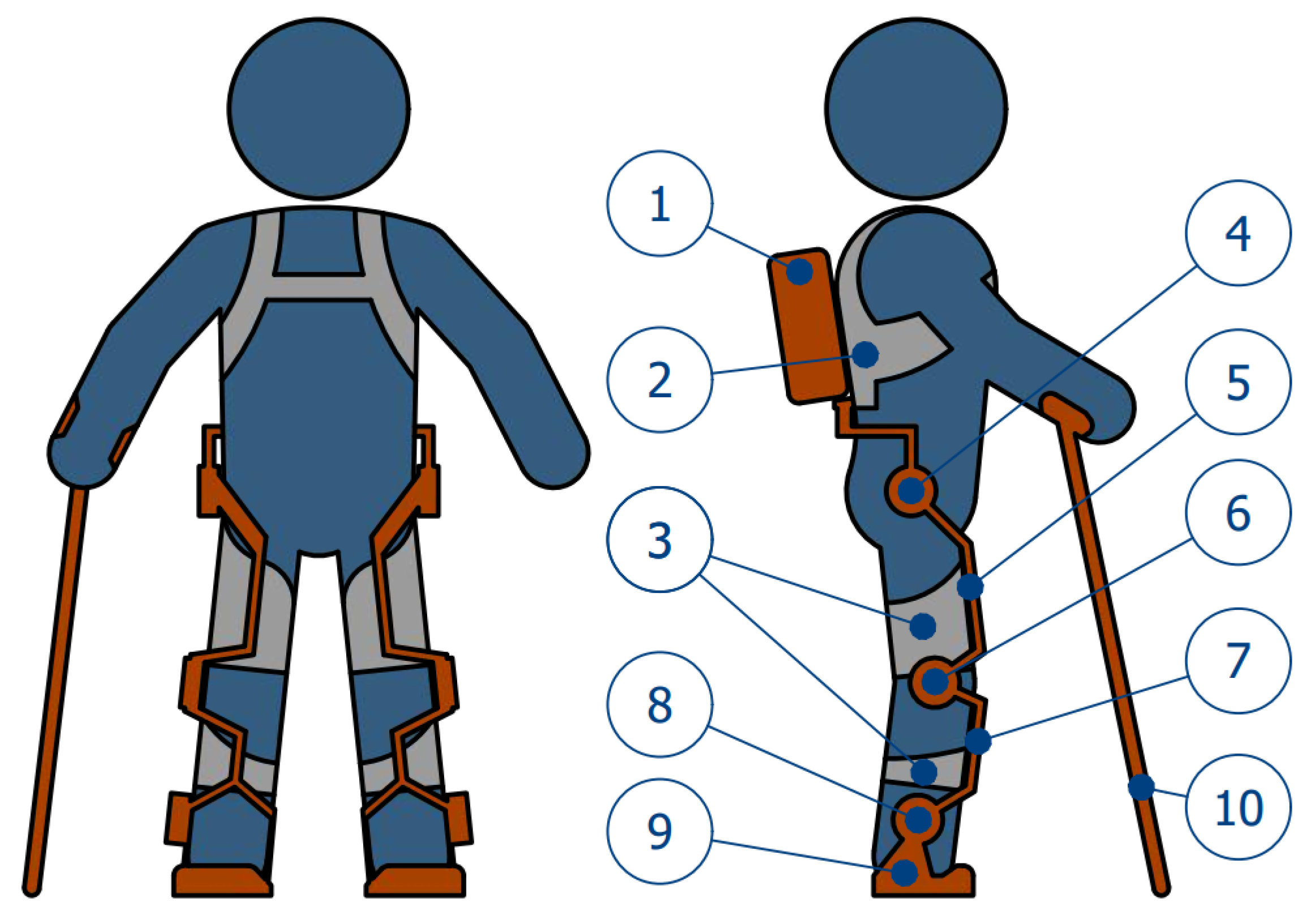
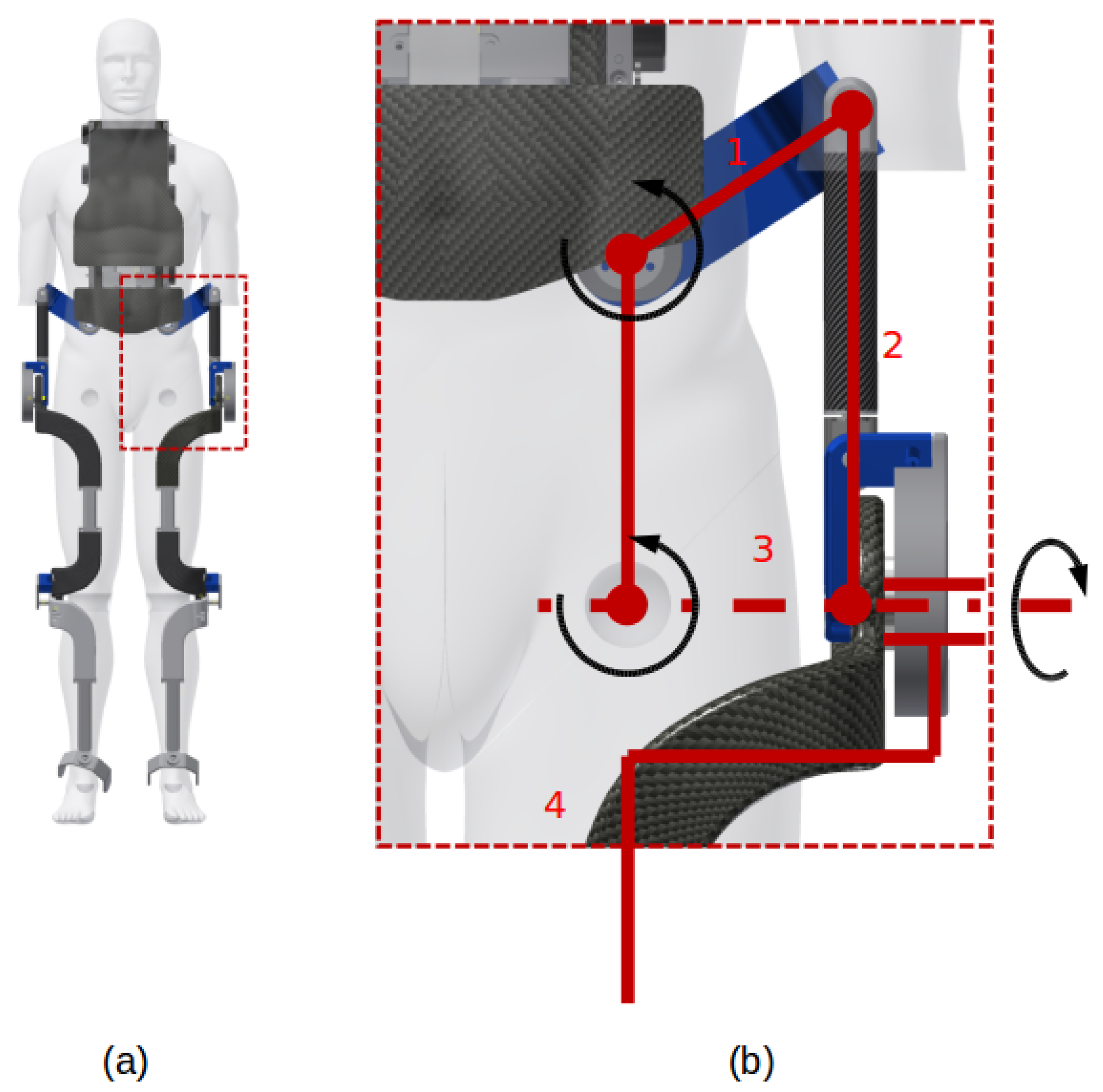
3.1. Conceptual Design

Since exoskeletons are worn by the user, they have an inherent requirement of compatibility with the anatomy and movement of the human body. Otherwise, they would disturb the activities they try to aid or improve. Furthermore, it is highly desirable that an exoskeleton not only be as thin and light as possible, but also comfortable and easy to wear. To illustrate the application of the method proposed in this work we will use the exoskeleton developed in the Laboratory of Biomechatronics of the Universidade de Sao Paulo, called ETMICAE (Exoesqueleto de Tronco e Membros Inferiores para Caminhada Autônoma Estável, in Portuguese), which means exoskeleton of the trunk and lower limbs for an autonomous stable gait. The ETMICAE was designed for applications in the areas of physiotherapy and research, for the purpose of rehabilitation and motor assistance of paraplegic people. Differently to most of the state of art exoskeletons, the attachments between the equipment and user at the limbs are frontal. In this way, it is possible to reduce the torsion caused by lateral exoskeleton attachments in order to improve the user comfort and to make it easier to wear, even with the concomitant use of a wheelchair. To reduce the swinging masses, the actuation is performed by cables, allowing to place the motors in the back of the body. An overview of the exoskeleton configuration is depicted in Figure 1.

There are several configurations of exoskeletons for rehabilitation varying the number of degrees of freedom according to their purpose [23]. However, in general, the actuated ones are in the sagittal plane of motion, preponderant in the walk. The ETMICAE has 7 degrees of freedom on each leg, distributed according to

Table 1. Number of dofs on each leg.

Joint	Dof	Actuated	Passive
Hip	3	Flex-extension	Rotation
		Adduction–abduction	Internal–external
Knee	1	Flex–extension	–
Ankle	2	Flex–extension	Inversion–eversion
Metatarsophalangeal	1	–	Flex–extension

. As it is intended to use just one crutch, the adduction–abduction dof is actuated to position the centre of mass on the support foot. Additionally, it has a passive degree of freedom at the foot, at the metatarsophalangeal joint, to improve the ground contact during the terminal stance phase.

The exoskeleton must be able to accommodate users from 1.55 m to 1.80 m tall and with a body mass up to 80 kg, who have trunk control and enough arm strength to transfer from a bed to a chair. Therefore, to position the joints properly, some adjustments are required for each individual. Moreover, due to the offset between the human and exoskeleton joint rotation axes, there occur movement misalignments that could cause singularities or even locking in the movement. Thus, mechanisms are required to compensate those misalignments. The mechanism used in the hip joint of ETMICAE for this purpose is shown in Figure 2. A four-bar linkage compensates the misalignment that would occur for the flexion–extension axis when the adduction–abduction is performed. Moreover, the exoskeleton joint for the adduction–abduction allows the user to sit comfortably.

3.2. Mobility Analysis

In order to determine the mobility of a substructure of the proposed lower limb exoskeleton, the Lie’s displacement group theory was employed [24,25]. Initially, the mechanical structure can be divided into two kinematic chains (Figure 3). The kinematic chain I, composed of links 0, 1, 2, 3 and 4, provides ${\mathcal{L}}_I(0,4)$ as the set of displacements

$${\mathcal{L}}_I(0,4)=Trans(\Delta x_{G_2}{\mathbf{i}}_0)\cup Trans(\Delta y_{G_2}{\mathbf{j}}_0)\cup Rot(\Delta q_3{\mathbf{k}}_3)\cup Rot(\Delta q_4{\mathbf{i}}_3)$$

(11)

On the other hand, the kinematic chain II, composed of links 0 and 4, is capable of performing the set of displacements ${\mathcal{L}}_{II}(0,4)$

$${\mathcal{L}}_{II}(0,4)=Rot(\Delta q_3{\mathbf{k}}_3)\cup Rot(\Delta q_4{\mathbf{i}}_3)$$

(12)

Therefore, from the intersection between the sets of displacements of the two chains, one can conclude that the independent displacements are

$$\mathcal{L}(0,4)={\mathcal{L}}_I(0,4)\cap {\mathcal{L}}_{II}(0,4)=Rot(\Delta q_3{\mathbf{k}}_3)\cup Rot(\Delta q_4{\mathbf{i}}_3)$$

(13)

which means that the whole system has 2 degrees of freedom.

4. The Exoskeleton Modelling

According to Figure 4, the substructure of the exoskeleton is assumed to have only three bodies, namely, links 1, 3 and 4. In Section 4.1, the kinematic variables are obtained, while in Section 4.2, the dynamic model is derived by applying the MMM method. Later, Section 4.3 explains how the dynamic model can be modified in order to consider the dynamic effects of link 2 and possible changes in the design parameters.

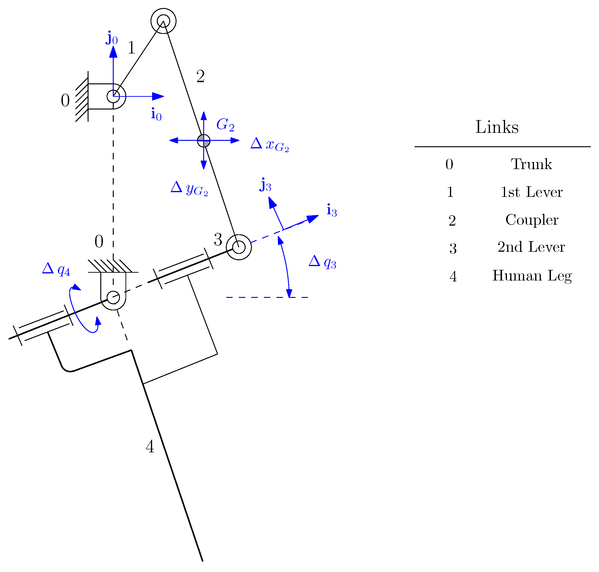
4.1. Kinematic Model

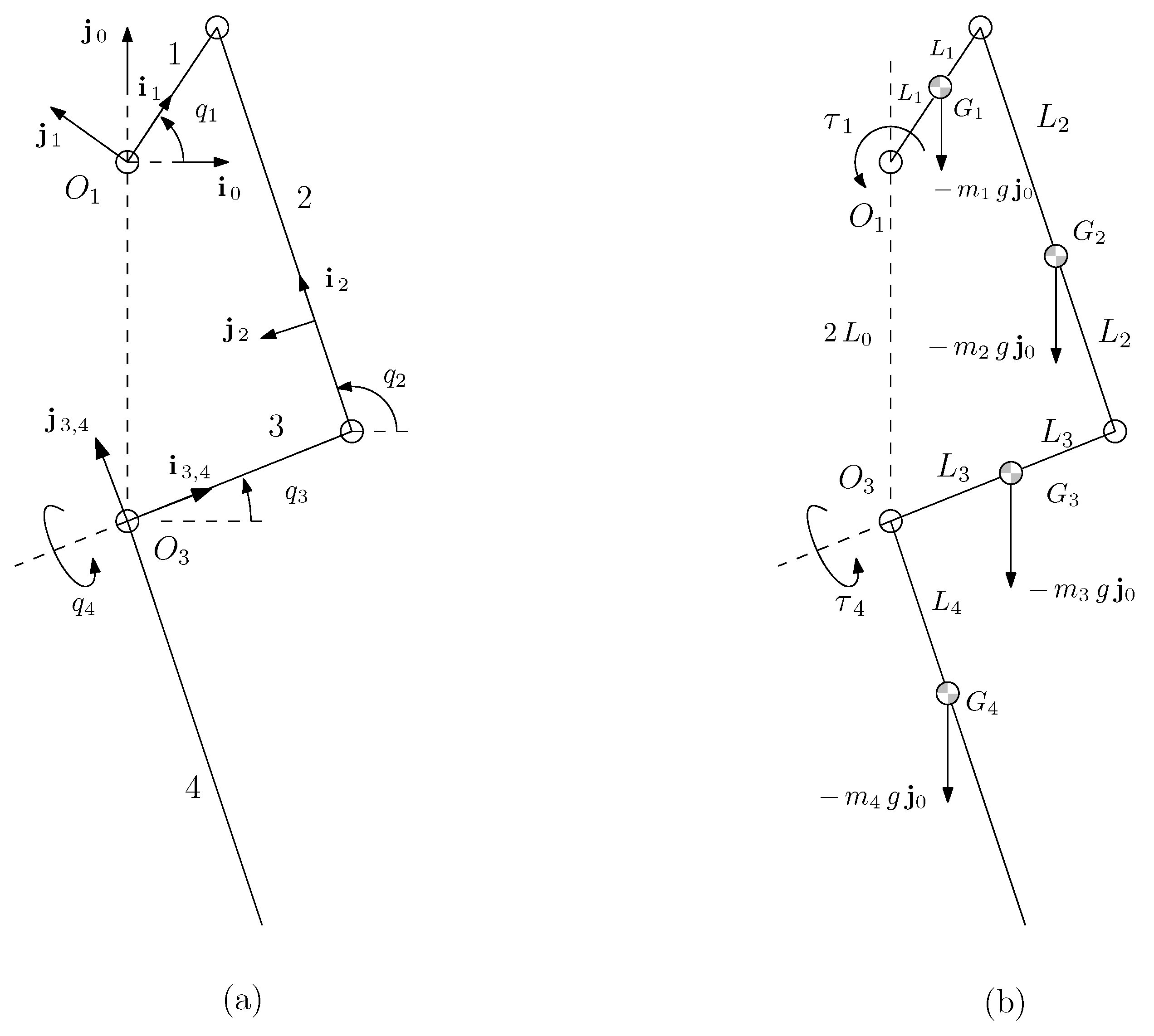
Due to the fact that one actuator drives link 1, while the other drives link 4 (Figure 5), the chosen generalised velocities are ${\dot{q}}_1$ and ${\dot{q}}_4$. Then, the total number of redundant kinematic variables n can be computed as follows,

$$n=\sum _{k=1,\ne 2}^4{\lambda }_k=12$$

For link 1, the velocities ${\mathbf{v}}_{G_1}$ and ${\mathit{\omega }}_1$ are

$${\mathbf{v}}_{G_1}=L_1{\dot{q}}_1{\mathbf{j}}_1=L_1{\dot{q}}_1\left[\begin{array}{c}-s_1\\ c_1\end{array}\right]=\left[\begin{array}{c}{}^0{v}_{G_{1x}}\\ {}^0{v}_{G_{1y}}\end{array}\right]=\left[\begin{array}{c}{u}_1\\ u_2\end{array}\right]$$

$${\mathit{\omega }}_1={\dot{q}}_1{\mathbf{k}}_1={}^1{\mathit{\omega }}_{1z}{\mathbf{k}}_1=u_3{\mathbf{k}}_1$$

For link 3, the velocities ${\mathbf{v}}_{G_3}$ and ${\mathit{\omega }}_3$ are

$${\mathbf{v}}_{G_3}=L_3{\dot{q}}_3{\mathbf{j}}_3=L_3{\dot{q}}_3\left[\begin{array}{c}-s_3\\ c_3\end{array}\right]=\left[\begin{array}{c}{}^0{v}_{G_{3x}}\\ {}^0{v}_{G_{3y}}\end{array}\right]=\left[\begin{array}{c}{u}_4\\ u_5\end{array}\right]$$

$${\mathit{\omega }}_3={\dot{q}}_3{\mathbf{k}}_3={}^3{\mathit{\omega }}_{3z}{\mathbf{k}}_3=u_6{\mathbf{k}}_3$$

For link 4, the velocities ${\mathit{\omega }}_4$ and ${\mathbf{v}}_{G_4}$ are

$${\mathit{\omega }}_4={\dot{q}}_3{\mathbf{k}}_3+{\dot{q}}_4{\mathbf{i}}_4={\dot{q}}_3{}^4{R}_3{}^3{\mathbf{k}}_3+{\dot{q}}_4{}^4{\mathbf{i}}_4={\dot{q}}_3\left[\begin{array}{ccc}1& 0& 0\\ 0& c_4& s_4\\ 0& -s_4& c_4\end{array}\right]\left[\begin{array}{c}0\\ 0\\ 1\end{array}\right]+{\dot{q}}_4\left[\begin{array}{c}1\\ 0\\ 0\end{array}\right]$$

$$=\left[\begin{array}{c}{\dot{q}}_4\\ {\dot{q}}_3{s}_4\\ {\dot{q}}_3{c}_4\end{array}\right]=\left[\begin{array}{c}{}^4{\mathit{\omega }}_{4x}\\ {}^4{\mathit{\omega }}_{4y}\\ {}^4{\mathit{\omega }}_{4z}\end{array}\right]=\left[\begin{array}{c}{u}_{10}\\ u_{11}\\ u_{12}\end{array}\right]$$

$${}^4{\mathbf{v}}_{G_4}={}^4{\mathit{\omega }}_4\times ({}^4{\mathbf{r}}_{G_4}-{}^4{\mathbf{r}}_{O_4})=\left[\begin{array}{ccc}0& -{}^4{\mathit{\omega }}_{4z}& {}^4{\mathit{\omega }}_{4y}\\ {}^4{\mathit{\omega }}_{4z}& 0& -{}^4{\mathit{\omega }}_{4x}\\ -{}^4{\mathit{\omega }}_{4y}& {}^4{\mathit{\omega }}_{4x}& 0\end{array}\right]\left[\begin{array}{c}0\\ -L_4\\ 0\end{array}\right]$$

$$=L_4\left[\begin{array}{c}{}^4{\mathit{\omega }}_{4z}\\ 0\\ -{}^4{\mathit{\omega }}_{4x}\end{array}\right]=L_4\left[\begin{array}{c}{\dot{q}}_3{c}_4\\ 0\\ -{\dot{q}}_4\end{array}\right]$$

$${}^0{\mathbf{v}}_{G_4}={}^0{R}_3{}^3{R}_4{}^4{\mathbf{v}}_{G_4}=\left[\begin{array}{ccc}{c}_3& -s_3& 0\\ s_3& c_3& 0\\ 0& 0& 1\end{array}\right]\left[\begin{array}{ccc}1& 0& 0\\ 0& c_4& -s_4\\ 0& s_4& c_4\end{array}\right]\left[\begin{array}{c}{\dot{q}}_3{c}_4\\ 0\\ -{\dot{q}}_4\end{array}\right]L_4$$

$$=\left[\begin{array}{c}{\dot{q}}_3{c}_4{c}_3-{\dot{q}}_4{s}_4{s}_3\\ {\dot{q}}_3{c}_4{s}_3+{\dot{q}}_4{s}_4{c}_3\\ -{\dot{q}}_4{c}_4\end{array}\right]L_4=\left[\begin{array}{c}{u}_7\\ u_8\\ u_9\end{array}\right]$$

By assuming $L_1$ = $L_3$, then $q_1$ = $q_3$ and the coupling matrix C becomes

$$C=\left[\begin{array}{c}{C}_1\\ C_3\\ C_4\end{array}\right]=\left[\begin{array}{cc}-s_1{L}_1& 0\\ c_1{L}_1& 0\\ 1& 0\\ & \\ -s_1{L}_1& 0\\ c_1{L}_1& 0\\ 1& 0\\ & \\ c_1{c}_4{L}_4& -s_1{s}_4{L}_4\\ s_1{c}_4{L}_4& c_1{s}_4{L}_4\\ 0& -c_4{L}_4\\ 0& 1\\ s_4& 0\\ c_4& 0\end{array}\right].$$

4.2. Dynamic Model

The dynamic model of the exoskeleton considers the inertial and gravitational forces of links 1, 3 and 4. In addition, the driving torques of actuators 1 and 4 are taken into account, which are, respectively, ${\tau }_1$ and ${\tau }_4$. Hence, the vector $\mathbf{f}$ can be calculated as follows,

$$\mathbf{f}=\left[\begin{array}{c}{\mathbf{f}}_1\\ {\mathbf{f}}_3\\ {\mathbf{f}}_4\end{array}\right]=\left[\begin{array}{c}-m_1{\dot{u}}_1\\ -m_1\left({\dot{u}}_2+g\right)\\ {\tau }_1-{\dot{u}}_3{I}_1\\ \\ -m_3{\dot{u}}_4\\ -m_3\left({\dot{u}}_5+g\right)\\ -{\dot{u}}_6{I}_3\\ \\ -m_4{\dot{u}}_7\\ -m_4\left({\dot{u}}_8+g\right)\\ -m_4{\dot{u}}_9\\ \left(I_{4y}-I_{4z}\right)u_{11}{u}_{12}-I_{4x}{\dot{u}}_{10}+{\tau }_4\\ -\left(I_{4x}-I_{4z}\right)u_{10}{u}_{12}-I_{4y}{\dot{u}}_{11}\\ -I_{4z}{\dot{u}}_{12}-\left(I_{4y}-I_{4x}\right)u_{10}{u}_{11}\end{array}\right]$$

From Equation (7), the dynamic equations are

$$\left[\begin{array}{ccc}{C}_1^T& C_3^T& C_4^T\end{array}\right]\left[\begin{array}{c}{\mathbf{f}}_1\\ {\mathbf{f}}_3\\ {\mathbf{f}}_4\end{array}\right]=\left[\begin{array}{c}0\\ 0\end{array}\right]$$

$$\left[\begin{array}{c}-m_4{s}_1{c}_4\left({\dot{u}}_8+g\right)L_4-m_4{c}_1{c}_4{\dot{u}}_7{L}_4-m_3{c}_1\left({\dot{u}}_5+g\right)L_1+\\ m_3{s}_1{\dot{u}}_4{L}_1-m_1{c}_1\left({\dot{u}}_2+g\right)L_1+m_1{s}_1{\dot{u}}_1{L}_1-{\dot{u}}_6{I}_3-{\dot{u}}_3{I}_1+\\ c_4\left(-I_{4z}{\dot{u}}_{12}-\left(I_{4y}-I_{4x}\right)u_{10}{u}_{11}\right)+s_4\left(-\left(I_{4x}-I_{4z}\right)u_{10}{u}_{12}-I_{4y}{\dot{u}}_{11}\right)+{\tau }_1\\ \\ m_4{c}_4{\dot{u}}_9{L}_4-m_4{c}_1{s}_4\left({\dot{u}}_8+g\right)L_4+m_4{s}_1{s}_4{\dot{u}}_7{L}_4+\left(I_{4y}-I_{4z}\right)u_{11}{u}_{12}-I_{4x}{\dot{u}}_{10}+{\tau }_4\end{array}\right]=\left[\begin{array}{c}0\\ 0\end{array}\right]$$

By assuming that $m_1=m_3$ and $I_1=I_3$,

$$\begin{array}{c}{\ddot{q}}_1(2m_1{L}_1^2+2I_1+m_4{L_4}^2{c_4}^2+I_{4y}{s_4}^2+I_{4z}{c_4}^2)+\\ 2{\dot{q}}_1{\dot{q}}_4(-m_4{L_4}^2-I_{4z}+I_{4y})c_4{s}_4+g(2m_1{L}_1{c}_1+m_4{L}_4{s}_1{c}_4)={\tau }_1\end{array}$$

$${\ddot{q}}_4(m_4{L_4}^2+I_{4x})+{{\dot{q}}_1}^2(m_4{L}_4^2+I_{4z}-I_{4y})c_4{s}_4+g{m}_4{L}_4{c}_1{s}_4={\tau }_4$$

4.3. Modifying the Dynamic Model

In order to take into account the effect of the gravitational force of link 2, the dynamic model needs to be modified. Then, the linear and angular velocities, ${\mathbf{v}}_{G_2}$ and ${\mathit{\omega }}_2$, can be calculated and three redundant variables, $u_{13},u_{14}$ and $u_{15}$ are added,

$${\mathbf{v}}_{G_2}=2L_1{\dot{q}}_1{\mathbf{j}}_1=2L_1{\dot{q}}_1\left[\begin{array}{c}-s_1\\ c_1\end{array}\right]=\left[\begin{array}{c}{}^0{v}_{G_{2x}}\\ {}^0{v}_{G_{2y}}\end{array}\right]=\left[\begin{array}{c}{u}_{13}\\ u_{14}\end{array}\right]$$

$${\mathit{\omega }}_2=0{\mathbf{k}}_2={}^2{\mathit{\omega }}_{2z}{\mathbf{k}}_2=u_{15}{\mathbf{k}}_2$$

Hence, the coupling matrix $C_2$ is

$$C_2=2\left[\begin{array}{cc}-s_1{L}_1& 0\\ c_1{L}_1& 0\\ 0& 0\end{array}\right]$$

The vector ${\mathbf{f}}_2$ is

$${\mathbf{f}}_2={\left[\begin{array}{ccc}0& -m_{2}g& 0\end{array}\right]}^T$$

Then, the dynamic equations become

$$\left[\begin{array}{cccc}{C}_1^T& C_2^T& C_3^T& C_4^T\end{array}\right]\left[\begin{array}{c}{\mathbf{f}}_1\\ {\mathbf{f}}_2\\ {\mathbf{f}}_3\\ {\mathbf{f}}_4\end{array}\right]=\left[\begin{array}{c}0\\ 0\end{array}\right]$$

$$\begin{array}{c}{\ddot{q}}_1(2m_1{L}_1^2+2I_1+m_4{L_4}^2{c_4}^2+I_{4y}{s_4}^2+I_{4z}{c_4}^2)+\\ 2{\dot{q}}_1{\dot{q}}_4(-m_4{L_4}^2-I_{4z}+I_{4y})c_4{s}_4+g(2m_1{L}_1{c}_1+2m_2{L}_1{c}_1+m_4{L}_4{s}_1{c}_4)={\tau }_1\end{array}$$

$${\ddot{q}}_4(m_4{L_4}^2+I_{4x})+{{\dot{q}}_1}^2(m_4{L}_4^2+I_{4z}-I_{4y})c_4{s}_4+g{m}_4{L}_4{c}_1{s}_4={\tau }_4$$

By assuming that the parameters $L_3$ and $L_1$ are distinct, the angular and linear velocities of links 2 and 3 must be recalculated,

$${\mathit{\omega }}_2={\dot{q}}_2{\mathbf{k}}_2={}^2{\mathit{\omega }}_{2z}{\mathbf{k}}_2$$

$${\dot{q}}_2={\dot{q}}_1\frac{2L_1}{2L_2}\frac{{\mathbf{j}}_1^T{\mathbf{i}}_3}{{\mathbf{j}}_2^T{\mathbf{i}}_3}={\dot{q}}_1\frac{L_1}{L_2}\left(\frac{-s_1{c}_3+c_1{s}_3}{-s_2{c}_3+c_2{s}_3}\right)={\dot{q}}_1\frac{L_1}{L_2}\frac{s_{1-3}}{s_{2-3}}={\dot{q}}_1\frac{L_1}{L_2}{\Delta }_2=u_{15}$$

$${\mathit{\omega }}_3={\dot{q}}_3{\mathbf{k}}_3={}^3{\mathit{\omega }}_{3z}{\mathbf{k}}_3$$

$${\dot{q}}_3={\dot{q}}_1\frac{2L_1}{2L_3}\frac{{\mathbf{j}}_1^T{\mathbf{i}}_2}{{\mathbf{j}}_3^T{\mathbf{i}}_2}={\dot{q}}_1\frac{L_1}{L_3}\left(\frac{-s_1{c}_2+c_1{s}_2}{-s_3{c}_2+c_3{s}_2}\right)={\dot{q}}_1\frac{L_1}{L_3}\frac{s_{2-1}}{s_{2-3}}={\dot{q}}_1\frac{L_1}{L_3}{\Delta }_3=u_6$$

$${\mathbf{v}}_{G_3}={\dot{q}}_3{L}_3{\mathbf{j}}_3={\dot{q}}_1{L}_1{\Delta }_3\left[\begin{array}{c}-s_3\\ c_3\end{array}\right]=\left[\begin{array}{c}{u}_4\\ u_5\end{array}\right]$$

$${\mathbf{v}}_{G_2}={\dot{q}}_{3}2L_3{\mathbf{j}}_3+{\dot{q}}_2{L}_2{\mathbf{j}}_2={\dot{q}}_1{L}_1\left(2{\Delta }_3{\mathbf{j}}_3+{\Delta }_2{\mathbf{j}}_2\right)={\dot{q}}_1{L}_1\left[\begin{array}{c}-2s_3{\Delta }_3-s_2{\Delta }_2\\ 2c_3{\Delta }_3+c_2{\Delta }_2\end{array}\right]=\left[\begin{array}{c}{}^0{v}_{G_{2x}}\\ {}^0{v}_{G_{2y}}\end{array}\right]=\left[\begin{array}{c}{u}_{13}\\ u_{14}\end{array}\right]$$

Hence, the coupling matrices $C_2$ and $C_3$ are

$$C_2=\left[\begin{array}{cc}{L}_1(-2s_3{\Delta }_3-s_2{\Delta }_2)& 0\\ L_1(2c_3{\Delta }_3+c_2{\Delta }_2)& 0\\ \frac{L_1}{L_2}{\Delta }_2& 0\end{array}\right]$$

$$C_3=\left[\begin{array}{cc}-s_3{L}_1{\Delta }_3& 0\\ c_3{L}_1{\Delta }_3& 0\\ \frac{L_1}{L_3}{\Delta }_3& 0\end{array}\right]$$

As a consequence, the dynamic equations become

$${\ddot{q}}_1\left(m_1{L}_1^2+I_1+(\frac{I_3}{L_3^2}+m_3)L_1^2{\Delta }_3^2+m_4{L}_4^2{c}_4^2+I_{4y}{s}_4^2+I_{4z}{c}_4^2\right)$$

$$+{\dot{q}}_1^2(\frac{I_3}{L_3^2}+m_3)L_1^2{\Delta }_3^2\left(\frac{c_{2-1}}{s_{2-1}}(\frac{L_1}{L_2}{\Delta }_2-1)+\frac{c_{2-3}}{s_{2-3}}(\frac{L_1}{L_3}{\Delta }_3-\frac{L_1}{L_2}{\Delta }_2)\right)$$

$$+{\dot{q}}_1{\dot{q}}_4\left(1+\frac{L_1}{L_3}{\Delta }_3\right)\left(I_{4y}-I_{4z}-m_4{L_4}^2\right)c_4{s}_4$$

$$+g{m}_1{L}_1{c}_1+g{m}_2{L}_1(2c_3{\Delta }_3+c_2{\Delta }_2)+g{m}_3{L}_1{\Delta }_3{c}_3+g{m}_4{L}_4{s}_3{c}_4={\tau }_1$$

$${\ddot{q}}_4\left(m_4{L_4}^2+I_{4x}\right)+{\dot{q}}_1^2\left(m_4{L}_4^2+(I_{4z}-I_{4y})\frac{L_1}{L_3}{\Delta }_3\right)c_4{s}_4\frac{L_1}{L_3}{\Delta }_3+g{m}_4{L}_4{c}_3{s}_4={\tau }_4$$

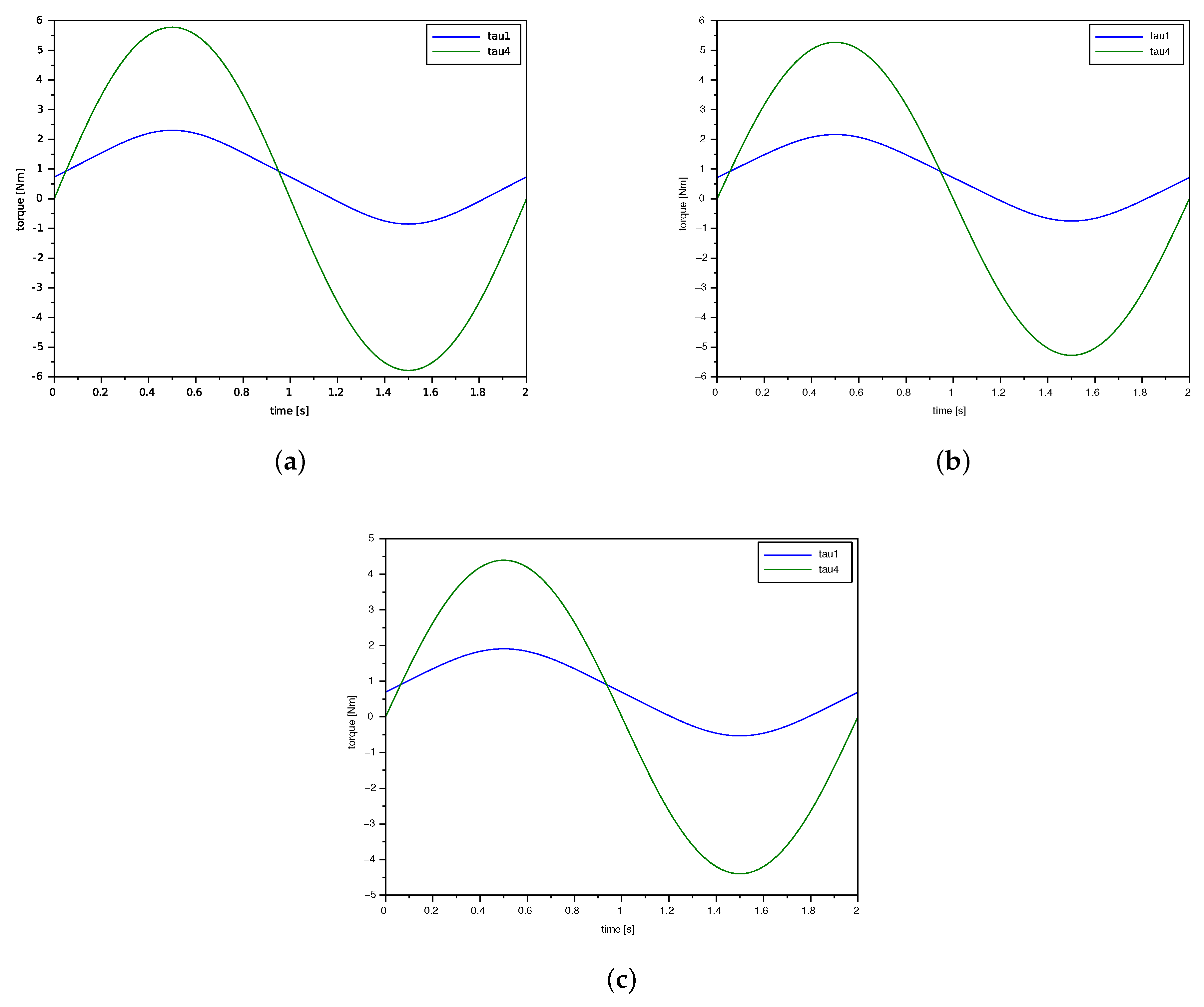
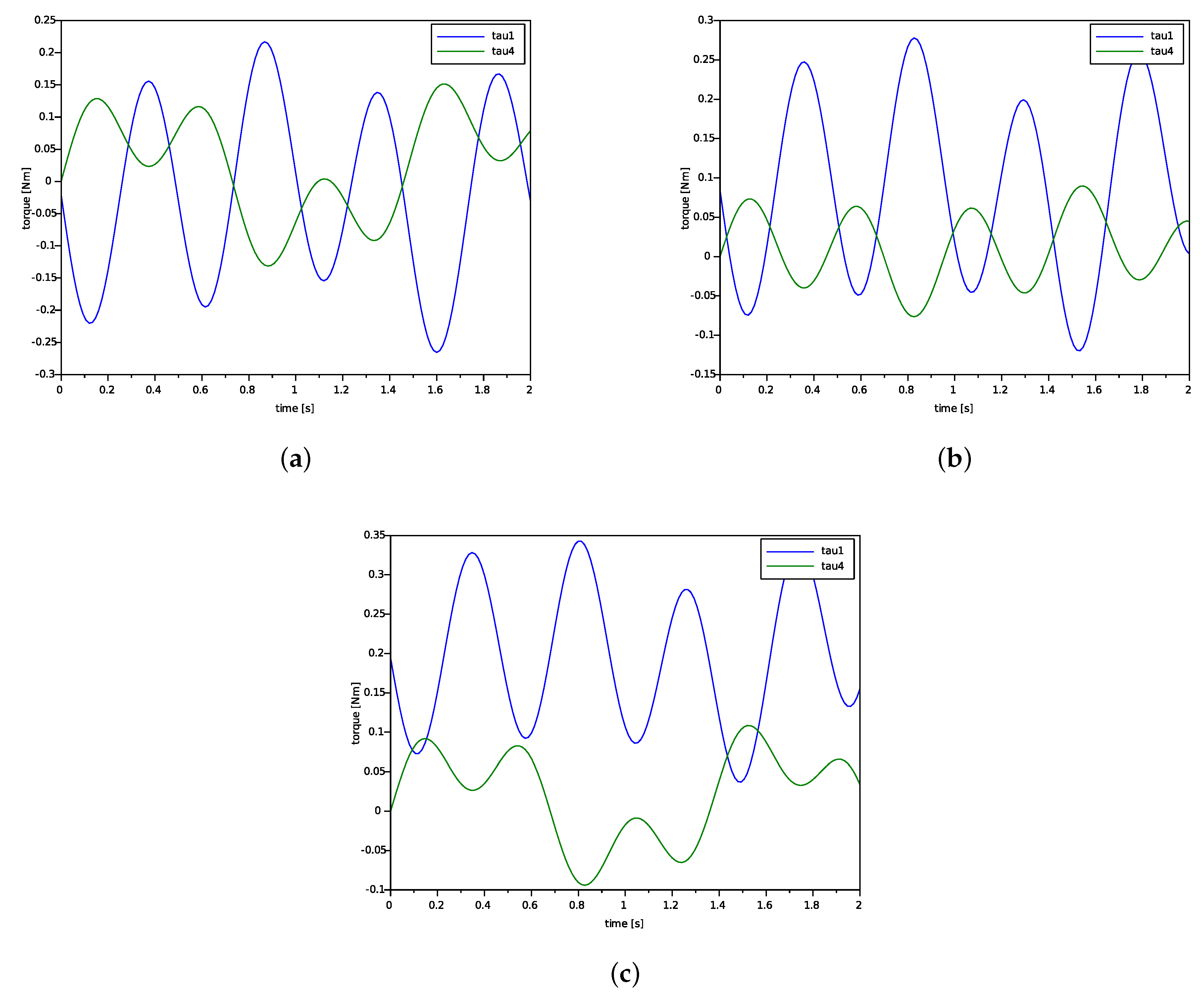
5. Simulations and Results

From the dynamic equations deduced in previous sections, some simulations were performed in order to evaluate the model consistency and to estimate the actuator torques as well.

Table 2. Selected parameters for the analyses.

	Link 1		Link 2		Link 3
$m_1\left(kg\right)$	0.18	$m_2\left(kg\right)$	0.15	$m_3\left(kg\right)$	0.2
$L_1\left(m\right)$	0.09	$L_2\left(m\right)$	0.2	$L_3\left(m\right)$	0.1
$I_1\left(kg{m}^2\right)$	0.00068	$I_2\left(kg{m}^2\right)$	0.0014	$I_3\left(kg{m}^2\right)$	0.00072
Link 4	$m_4\left(kg\right)$	$L_4\left(m\right)$	$I_{4x}\left(kg{m}^2\right)$	$I_{4y}\left(kg{m}^2\right)$	$I_{4z}\left(kg{m}^2\right)$
1.8 m, 80 kg	13.3	0.36	0.819	0.0062	0.819
1.7 m, 60 kg	11.1	0.36	0.51	0.006	0.51
1.6 m, 50 kg	9.3	0.34	0.38	0.006	0.38

shows the selected parameters for the exoskeleton and a typical male adult (80 kg, 1.80 m) user [26]. In addition, we tested the application of this method to change the design parameters to adapt to other users with other heights and weights (60 kg, 1.70 m) and a shorter one (50 kg, 1.60 m) [27].

5.1. First Simulation: Inverse Dynamics

For the first simulation, the input motions for the exoskeleton were prescribed, namely, $q_1\left(t\right)$ and $q_4\left(t\right)$. Such functions were chosen as sinusoidal functions whose amplitudes was equal to 5 and 15 degrees, respectively, and both periods were equal to 2 s. Hence, the torques ${\tau }_1$ and ${\tau }_4$ for the motion cycle can be calculated. Figure 6 shows that the actuator torques were both periodic functions whose period was equal to 2 s. In addition, the maximum values of ${\tau }_1$ and ${\tau }_4$ were, respectively, for 1.8 m 80 kg: 2.3 and 5.8 Nm, for 1.7 m 60 kg: 2.2 and 5.3 Nm and for 1.6 m 50 kg: 1.9 and 4.4 Nm.

5.2. Second Simulation: Direct Dynamics

For the second simulation, the actuator torques were considered null while the initial conditions were $q_1\left(0\right)=$ 5 deg, $q_4\left(0\right)=$ 15 deg, ${\dot{q}}_1\left(0\right)=$ 0 rad/s, ${\dot{q}}_4\left(0\right)=$ 0 rad/s. Figure 7 shows the generalized coordinates and velocities during a 5 s simulation. One can notice that the simulated system has a conservative behaviour once there is no dissipative effects such as friction or damping. Regarding the oscillation around the ${\mathbf{k}}_0$-axis, the equilibrium position is approximately $q_1$ = −1.03 deg, which is expected since the exoskeleton behaves as an unbalanced pendulum. Moreover, there are two natural periods associated to this free vibration for the 1.8 m, 80 kg simulation, which correspond to 1.53 ($q_1$) and 1.46 s ($q_4$). Similarly, the natural periods for 1.7 m, 60 kg were: 1.47 and 1.40 s, while for 1.6 m, 50 kg they were 1.43 and 1.36 s, for $q_1$ and $q_4$, respectively.

5.3. Third Simulation: Inverse Dynamics

For the third simulation, the input motions for the exoskeleton were prescribed, namely, $q_1\left(t\right)$ and $q_4\left(t\right)$. Such functions were also chosen to be sinusoidal with amplitudes equal to 6 and 15 degrees, and periods equal to 1.53 and 1.46 s, respectively. Hence, the actuator torques ${\tau }_1$ and ${\tau }_4$ for the motion cycle can be recalculated. Figure 8 shows that the maximum absolute values for ${\tau }_1$ and ${\tau }_4$ reached 0.27 Nm and 0.15 Nm, respectively. Finally, the maximum torques ${\tau }_1$ and ${\tau }_4$ for 1.7 m, 60 kg were, respectively, 0.28 and 0.09 Nm, while for 1.6 m, 50 kg they were 0.34 and 0.11 Nm.

Consequently, it can be noted that if the input motions take into account the natural frequencies of the system, the actuator torques can be significantly reduced.

6. Conclusions

In this article we presented a dynamic modelling approach based on the Modular modelling methodology (MMM) for the development of exoskeletons. Initially, the conceptual design of a lower limb exoskeleton was presented. Then, the kinematic and dynamic models of a substructure of the exoskeleton were calculated. In addition, performed simulations demonstrated the model consistency and the actuator torques estimation.

The MMM provides an easy procedure to obtain the dynamic model as a first step to address some challenges in exoskeleton design, such as real time control, sensor signal fusion or user intent detection. In this respect, we note that the MMM method has several contributions: it is not only suitable for modelling exoskeletons but also has advantages over other previous approaches in terms of ease of building the dynamic model and modifying it as well.

In order to illustrate an application of this method, we performed three simulations for different types of users to show that it is possible to easily adjust the exoskeleton parameters to different users. Therefore, this method can help the exoskeleton designer during the synthesis process, facilitating the definition of the parameters, the actuator selection and the model-based control simulations.

References

1. Pons, J.L. Wearable Robots: Biomechatronic Exoskeletons; John Wiley & Sons: Hoboken, NJ, USA, 2008. [Google Scholar]
2. Souza, R.S.; Sanfilippo, F.; Silva, J.R.; Forner-Cordero, A. Modular exoskeleton design: Requirement engineering with KAOS. In Proceedings of the IEEE International Conference on Biomedical Robotics and Biomechatronics (BioRob), Singapore, 26–29 June 2016; pp. 978–983. [Google Scholar]
3. Perry, J.C.; Rosen, J. Design of a 7 degree-of-freedom upper-limb powered exoskeleton. The First IEEE/RAS-EMBS International Conference on Biomedical Robotics and Biomechatronics. BioRob 2006, 2006, 805–810. [Google Scholar]
4. Apkarian, J.; Naumann, S.; Cairns, B. A three-dimensional kinematic and dynamic model of the lower limb. J. Biomech. 1989, 22, 143–155. [Google Scholar] [CrossRef]
5. Miranda, A.B.W. Exoesqueleto Robótico de Membro Superior com três Graus de Liberdade Ativos. Master’s Thesis, University of Sao Paulo, Sao Paulo, Brazil, 2014. [Google Scholar]
6. Hogan, N. Impedance Control: An Approach to manipulation: Part I, Part II, Part III. J. Dyn. Syst. Meas. Control 1985, 107, 1–24. [Google Scholar] [CrossRef]
7. Zoss, C.A.; Kazerooni, H.; Chu, A. Biomechanical Design of the Berkeley Lower Extremity exoskeleton (BLEEX). IEEE/ASME Trans. Mechatron. 2006, 11, 128–138. [Google Scholar] [CrossRef]
8. Guizzo, E.; Goldstein, H. The Rise of the Boots; IEEE Spectrum: New York, NY, USA, 2005; pp. 52–56. [Google Scholar]
9. Kazerooni, H.; Steger, R. The Berkeley lower extremity exoskeleton. J. Dyn. Syst. Meas. Control Trans. ASME 2006, 128, 14–25. [Google Scholar] [CrossRef]
10. Acosta-Marquez, C.; Bradley, D.A. The Analysis, Design and Implementation of a Model of an exoskeleton to Support Mobility. In Proceedings of the IEEE 9th International Conference on Rehabilitation Robotics, Chicago, IL, USA, 28 June–1 July 2005; pp. 99–102. [Google Scholar]
11. Altuzarra, O.; Eggers, P.M.; Campa, F.; Roldan-Paraponiaris, C.; Pinto, C. Dynamic modelling of lower-mobility parallel manipulators using the Boltzmann-Hammel equations. In Mechanisms, Transmissions and Applications; Springer: Berlin/Heidelberg, Germany, 2015; pp. 157–165. [Google Scholar]
12. Featherstone, R. Rigid Body Dynamics Algorithms; Springer: Berlin/Heidelberg, Germany, 2008; 272p. [Google Scholar]
13. Tsai, L.-W. Robot Analysis: The Mechanics of Serial and Parallel Manipulators; Wiley: New York, NY, USA, 1999. [Google Scholar]
14. Anam, K.; Al-Jumaily, A.A. Active exoskeleton Control Systems: State of the Art. Procedia Eng. 2012, 41, 988–994. [Google Scholar] [CrossRef] [Green Version]
15. Agrawal, S.K.; Banala, S.K.; Fattah, A.; Sangwan, V.; Krishnamoorthy, V.; Scholz, J.P.; Hsu, W.-L. Assessment of Motion of a Swing Leg and Gait Rehabilitation With a Gravity Balancing exoskeleton. IEEE Trans. Neural Syst. Rehabil. Eng. 2007, 15, 410–420. [Google Scholar] [CrossRef] [PubMed]
16. Collins, S.H.; Wiggin, M.B.; Sawicki, G.S. Reducing the energy cost of human walking using an unpowered exoskeleton. Nature 2015, 522, 212–215. [Google Scholar] [CrossRef] [PubMed] [Green Version]
17. Baruh, H. Analytical Dynamics; WCB/Mc Graw Hill: New York, NY, USA, 1999. [Google Scholar]
18. Kane, T.R.; Levinson, D.A. Dynamics: Theory and Applications; Mc Graw Hill: New York, NY, USA, 1985. [Google Scholar]
19. Orsino, R.M.M. A Contribution on Modelling Methodologies for Multibody Systems. Ph.D. Thesis, Escola Politécnica-University of São Paulo, São Paulo, Brazil, 2016; 213p. [Google Scholar]
20. Orsino, R.M.M.; Hess-Coelho, T.A. A contribution for developing more efficient dynamic modelling algorithms of parallel robots. Int. J. Mech. Robot. Syst. 2013, 1, 15–34. [Google Scholar] [CrossRef]
21. Orsino, R.M.M.; Hess-Coelho, T.A. A contribution on the modular modelling of multibody systems. Proc. R. Soc. A 2015, 471, 20150080. [Google Scholar] [CrossRef]
22. Hess-Coelho, T.A.; Orsino, R.M.M.; Malvezzi, F. Modular modelling methodology applied to the dynamic analysis of parallel mechanisms. Mech. Mach. Theory 2021, 161, 104332. [Google Scholar] [CrossRef]
23. Young, A.J.; Ferris, D.P. State of the Art and Future Directions for Lower Limb Robotic exoskeletons. IEEE Trans. Neural Syst. Rehabil. Eng. 2017, 25, 171–182. [Google Scholar] [CrossRef] [PubMed]
24. Hervé, J.M. The Lie group of rigid body displacements, a fundamental tool for mechanism design. Mech. Mach. Theory 1999, 34, 719–730. [Google Scholar] [CrossRef]
25. Angeles, J. Qualitative Synthesis of Parallel Manipulators. ASME J. Mech. Des. 2004, 126, 617–624. [Google Scholar] [CrossRef]
26. Winter, D.A. Biomechanics and Motor Control of Human Movement; Wiley: Hoboken, NJ, USA, 2009; 370p. [Google Scholar]
27. Winter, D.A. Adjustments to Zatsiorsky-Seluyanov’s segment inertia parameters. J. Biomech. 1996, 29, 1223–1230. [Google Scholar]
Figure 1. Exoskeleton components: (1) power pack; (2) trunk attachments; (3) limbs attachments; (4) hip joint; (5) upper leg frame; (6) knee joint; (7) lower leg frame; (8) ankle joint; (9) foot frame; (10) instrumented crutch.
Machines 10 00248 g001
Figure 2. CAD model: (a) exoskeleton attached to the trunk and lower limbs; (b) detailed view of links and joints.
Machines 10 00248 g002
Figure 3. The kinematic diagram of a substructure of the exoskeleton for the lower limb.
Machines 10 00248 g003
Figure 4. The system S: a four-bar linkage (bodies 1, 3) and the human lower limb (body 4).
Machines 10 00248 g004
Figure 5. Model conventions: (a) frames and variables; (b) centres of mass, gravitational forces and torques.
Machines 10 00248 g005
Figure 6. Inverse dynamics: torques of actuators 1 ( τ 1 : tau1) and 4 ( τ 4 : tau4) simulated for subjects of different heights and weights: (a) 1.8 m and 80 kg; (b) 1.7 m and 60 kg; (c) 1.6 m and 50 kg.
Machines 10 00248 g006
Figure 7. Direct dynamics: generalized coordinates and velocities of joints 1 ( q 1 , d q 1 / d t ) and 4 ( q 4 , d q 4 / d t ) simulated for subjects of different heights and weights: (a) 1.8 m and 80 kg; (b) 1.7 m and 60 kg; (c) 1.6 m and 50 kg.
Machines 10 00248 g007
Figure 8. Inverse dynamics: torques of actuators 1 ( τ 1 : tau1) and 4 ( τ 4 : tau4) simulated for subjects of different heights and weights: (a) 1.8 m and 80 kg; (b) 1.7 m and 60 kg; (c) 1.6 m and 50 kg.
Machines 10 00248 g008