Abstract
Certain progress has been made in fault diagnosis under cross-domain scenarios recently. Most researchers have paid almost all their attention to promoting domain adaptation in a common space. However, several challenges that will cause negative transfer have been ignored. In this paper, a reweighting method is proposed to overcome this difficulty from two aspects. First, extracted features differ greatly from one another in promoting positive transfer, and measuring the difference is important. Measured by conditional entropy, the weight of adversarial losses for those well aligned features are reduced. Second, the balance between domain adaptation and class discrimination greatly influences the transferring task. Here, a dynamic weight strategy is adopted to compute the balance factor. Consideration is made from the perspective of maximum mean discrepancy and multiclass linear discriminant analysis. The first item is supposed to measure the degree of the domain adaptation between source and the target domain, and the second is supposed to show the classification performance of the classifier on the learned features in the current training epoch. Finally, extensive experiments on several bearing fault diagnosis datasets are conducted. The performance shows that our model has an obvious advantage compared with other common transferring algorithms.
1. Introduction
Bearinga are one of the most important components of all mechanical systems, and their healthy working state is the basic guarantee for all kinds of machines to engage in production [1,2,3,4,5]. With the continuous progress of measurement technology and the development of Internet of Things technology [6], massive data measured through sensors are available, and bearing diagnosis methods based on signal analysis or machine learning have made great progress in recent work [7,8,9,10]. Among fault diagnosis methods based on signal analysis, common feature extraction methods include wavelet transform, spectral analysis, empirical mode decomposition, and fast Fourier transform [11,12,13,14]. Feng et al. investigated the correlation between tribological features of abrasive wear and fatigue pitting in gear meshing and constructed an indicator of vibration cyclostationarity (CS) to identify and track wear evolution [15]. Cédric Peeters et al. derived blind filters using constructed envelope spectrum sparsity indicators and proposed an effective method of fault detection in rotating machinery [16]. In addition, the methods based on machine learning and deep learning are more and more widely used because they do not rely on rich expert experience and can learn complex nonlinear relationships effectively [17]. The common models among them are deep neural networks, sparse coding, and Bayesian analysis, which optimize the parameters of classifiers by utilizing labeled historical fault data [18,19,20].
Although samples from unlabeled test datasets can often be effectively diagnosed by these methods, most of them are usually based on an ideal assumption that training datasets and test datasets are collected from the same part of the same machine and are quite similar in terms of data distribution [21]. Real world conditions are often very different from ideal ones because obtaining vibration data with labels from critical parts of some machines is hard or even impossible [22]. Furthermore, collecting data samples from each machine and labeling them manually cost a large amount of time and money [23]. Hence, several training datasets can only be collected from another part of the same machine or from other similar but different scenarios [24]. This kind of bearing fault diagnosis task with training data and test data from different datasets is usually called cross-domain fault diagnosis by researchers. Intrinsic discrepancies are observed in the data distribution between training datasets (source domain) with labels and test datasets (target domain) without labels. The discrepancies between source domain and target domain always have an adverse impact on the diagnostic accuracy, which is the main difficulty of cross-domain diagnosis tasks. Domain adaptation is the main strategy to solve this difficulty at present, which means making knowledge from the source domain useful for the target task by eliminating the distribution discrepancies between two domains.
To bridge the gap between the two domains in cross-domain diagnosis tasks and avoid the deterioration of performance of source data classifier on discrepant target data, several transfer learning methods based on domain adaptation have been developed in recent studies [25,26]. The common strategy of transfer learning methods based on domain adaptation is to train a domain-invariant classifier by eliminating the distribution mismatch between source and target domains [27,28]. To reduce the distribution mismatch between the two domains, distance matching methods and adversarial learning models are two main types of strategies. As for the former, maximum mean discrepancy (MMD) [3] is widely applied for distance measurement. For a better, faster computation, multikernel maximum mean discrepancy (MK-MMD) is proposed [29]. For instance, Xie et al. trained a domain-invariant classifier for cross-domain gearbox fault diagnosis by transfer component analysis (TCA) technology [30]. The latter kind of methods train a domain-invariant classifier through adversarial training between domains inspired from the strategy of generative adversarial network (GAN) [31]. In adversarial domain adaptation methods, the discriminator is responsible for distinguishing whether the feature produced by the feature extractor comes from the source domain or the target domain, whereas the feature extractor tries to obtain features that can not be distinguished by the discriminator. The competition between them drives them to promote their performance until the source domain features and target domain features are indistinguishable. A domain-invariant classifier that can be applied in source datasets and target datasets is then obtained.
In addition to marginal distribution alignment methods based on distance matching and adversarial training, conditional distribution alignment for unsupervised bearing health status diagnosis has been recently considered by many researchers. For example, Li et al. used the over fitting of various classifiers in a proposed adversarial multiclassifier model to improve class-level alignment [32]. Qian et al. introduced a novel soft label strategy to assist joint distribution alignment of fault source and target domain datasets [33]. Zhang et al. combined a novel subspace alignment model with JDA to achieve joint distribution alignment in fault diagnosis of rolling bearings under varying working conditions [34]. Wu et al. utilized joint distribution adaptation and a long-short term memory recurrent neural network model simultaneously to achieve domain adaptation under the condition of unbalanced bearing fault data [35]. Yu et al. proposed an effective simulation data-based domain adaptation strategy for intelligent fault diagnosis in which conditional and marginal distribution alignment is achieved between source data from the simulation model and target data from mechanical equipment in the actual field [36]. Moreover, Kuniaki Saito et al. proposed a novel maximum classifier discrepancy (MCD) to reduce the decision boundary of the classifier and achieved better classification performance [37]. Li et al. measured the completion degree of classification by employing a criterion based on linear discriminant analysis (LDA) to enhance the performance of the classifier on the target domain [38]. Yu et al. quantitatively measured the relative importance of marginal and conditional distributions of two domains and dynamically extracted domain-invariant features in a proposed novel dynamic adversarial adaptation network (DAAN) [39].
Although these transfer learning methods have made some progress in cross-domain bearing fault diagnosis, there are still some challenges that will cause negative transfer. Positive transfer means the knowledge learned from the source domain can effectively improve the performance of the model in the target domain. In contrast, the learning behaviour will be called negative transfer [40,41] when the knowledge from the source domain hinders the performance of learning in the target task. Obviously, it should be avoided in cross-domain diagnosis tasks. However, these difficulties that may lead to negative transfer have not received sufficient attention from previous researchers. The two main problems leading to negative transfer in cross-domain bearing fault diagnosis are as follows. First, some samples with poor transferability have not received as much attention as they deserve, which will lead to negative transfer. Almost all the existing domain adaptation models assume that all the data have the same influence. Certainly, this assumption does not hold in many real-world scenarios. Some sample data are more difficult to align because they are far from the distribution center when there is some noise in the measurement environment or under non-stationary conditions [42,43]. If each sample has the same weight in the domain adaptation training, achieving a good conditional distribution alignment will be difficult no matter how many training epochs are taken. Moreover, with the continuous updating of model parameters, the good adaptation performance of features from samples with strong transferability will be destroyed. At this stage, negative transfer occurs.
Second, the imbalance between the classifier training and domain adaptation may also cause negative transfer. Training of the fault classifier and the domain adaptation process are carried out simultaneously in most previous models, but the relationship between them is ignored and the two processes are considered independently. Indeed, excessive adaptation is likely to cause the failure of a diagnostic classifier, whereas over completion of classifier training could cause domain mismatch [44]. Both processes influence the diagnosis accuracy, that is, the over/under completion of any of the two processes leads to negative transfer. From the above analysis, we can see that there is a strong motivation to establish a more advanced method to solve the two challenges that may cause negative transfer in cross-domain fault diagnosis.
In order to solve the above challenges in the field of cross-domain fault diagnosis, a novel DRDA method is proposed in this paper. To address the negative transfer caused by some samples with poor transferability, a soft reweighting strategy inspired by curriculum learning and conditional information entropy is proposed. Such an indicator can well measure the adaption performance of each sample in real time to provide more attention to poorly aligned samples. After proper weight adjustment, the clustering of source and target domain datasets are strengthened, thus, the conditional distribution alignment can also be improved. To address the negative transfer caused by the imbalance between the classifier training and domain adaptation, a balance factor is introduced in our method to strike a balance between them and obtain a higher accuracy in the final diagnosis on the target domain dataset. Specifically, MMD is used as an estimator to observe the degree of domain adaptation. The factor based on linear discriminant analysis (LDA) [38] was proposed to estimate the degree of classifier training. An effective balance factor can then be constructed by combining these two items. Sufficient verification experiments demonstrate that our model outperforms state-of-the-art methods.
The main contributions of our work are as follows.
- 1
- A novel dynamic reweighted domain adaptation method is proposed to address challenges that will cause negative transfer in cross-domain bearing fault diagnosis. A reweighted adversarial loss strategy is introduced in DRDA to eliminate negative transfer caused by samples with poor transferability in cross-domain bearing fault diagnosis.
- 2
- A powerful balance factor is constructed in the proposed method to eliminate negative transfer caused by the imbalance between the classifier training and domain adaptation in cross-domain bearing fault diagnosis.
This paper is organised into the following sections. The preliminary concept is introduced in Section 2, including the problem description and a brief introduction to the domain adversarial learning and maximum classifier discrepancy theories. In Section 3, the proposed DRDA model for cross-domain diagnosis is introduced in detail. Section 4 presents and analyzes the diagnosis performance on cross-location and cross-speed cases. Finally, this article is concluded in Section 5.
2. Principle Knowledge
2.1. Problem Description
Our work mainly focuses on bearing health status diagnosis in cross-domain scenarios and aims to develop a transferable diagnosis model with strong generalization that can effectively combat negative transfer and identify fault types corresponding to the target domain samples accurately utilizing the knowledge learned from samples of the source domain. Thus, our paper is based on the following several reasonable hypotheses:
- 1
- Massive bearing source domain datasets with labels and target domain datasets without labels are available for domain adaptation and fault diagnosis.
- 2
- Although most of the samples from the two domains are similar to one another in terms of data distribution, several are not and are more difficult to align.
To study bearing health status diagnosis for bearing datasets from two different domains, this paper utilizes two industrial transfer scenarios:
- 1
- Bearing data from different locations of the same mechanical system are used as target datasets for cross-location domain adaptation.
- 2
- Bearing data from the same mechanical system under different rotation speed conditions are used as target datasets for cross-speed domain adaptation.
In this paper, the source dataset is denoted as , its label is denoted as , and represents the target domain dataset. Superscript s represents the source domain data, and t represents the target domain data. This work focuses on four kinds of bearing health status: ball fault (BF), healthy (H), inner race fault (IF), and outer race fault (OF). In this paper, the structures of modules with the same name in different methods are exactly the same, so the same modules in different methods are uniformly represented by unified symbols (feature extractor: , classifier: , domain discriminator: ). Details of the structure and parameters of these modules are shown in the Figure 1.
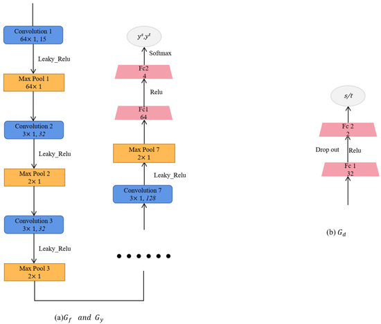
Figure 1.
The structure and parameters of the feature generator , fault classifier , and domain discriminator in proposed DRDA and other comparison methods.
2.2. Domain Adversarial Learning
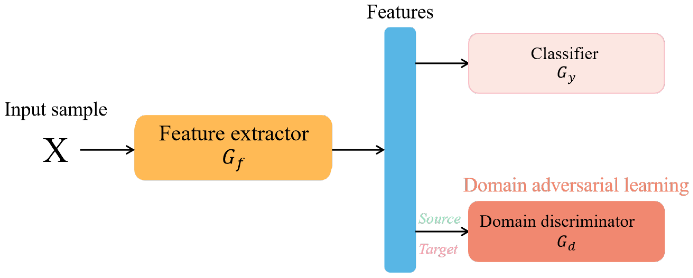
The main ideal of adversarial domain adaptation is to apply the min-max optimization strategy of GAN to extract domain-invariant features [45]. The basic structure of the adversarial domain adaptation network is shown in Figure 2.

Figure 2.
The structure of adversarial domain adaptation.
This model has three main components: A feature extractor (), a health status classifier (), and a discriminator (). The expressions , , and are the parameters of , , and , respectively. The parameters of the feature extractor and the discriminator are trained by samples from the source dataset and the target dataset, whereas the classifier is trained only on the source domain examples with labels. Specifically, the goal of the discriminator is to discern whether the features obtained by the feature extractor come from the source domain or the target domain, whereas the feature extractor aims to gain domain-invariant features that cannot be distinguished by the discriminator. The updating of parameters will eventually converge to an optimal equilibrium state, where the loss of the discriminator reaches its maximum corresponding to and minimum corresponding to . The loss can be expressed as follows:
where and are the number of samples in the source domain and target domain, respectively; is the classifier cross-entropy loss, and is the adversarial loss of the domain discriminator; is the label generated by the discriminator to represent the domain of input data (1 represents the target domain and 0 represents the source domain); and is a parameter with the function of trade-off. When the iterative process converges to the optimal state, the parameters satisfy Equation (2):
Thus, the domain adaptation can be achieved by the counterbalance of adversarial training.
2.3. Maximum Classifier Discrepancy (MCD)
The main goal of MCD is to narrow the decision boundary of the classification and eliminate the misclassification of samples whose features are near to the boundary in the feature space [37]. As shown in Figure 3, this model mainly consists of three modules: a feature extractor () and two classifiers (, ). The feature extractor is optimized to obtain features that could minimize the discrepancy of predictions given by the two classifiers. Discrepancy loss is defined as follows:
where c is the total number of all health status classes and equals 4 in this paper; , denote probability output of , for class k, respectively. The selection of the norm is crucial to the final results and -norm is adopted, as in the original paper. In MCD, min-max optimizing class discrepancy is a core procedure. First, the feature generator () is fixed to maximize discrepancy loss. Next, the two classifiers and are fixed to minimize discrepancy loss. Such min-max optimization procedures are all towards target samples, and source samples are only trained by the fault classifier’s cross entropy loss L. The optimization details can be expressed as follows:

Figure 3.
The structure of the maximum classifier discrepancy model, where is the feature extractor, and and are two classifiers.
3. Proposed Method
For a more robust and positive transfer, this paper introduces two reweighting strategies from two perspectives. First, adversarial loss is reweighted from the perspective of each sample. Second, a balance between domain adaptation and discrimination is made from the perspective of the whole dataset. In this section, the method, which mainly consists of four parts, will be explained in detail.
3.1. Expanding MCD
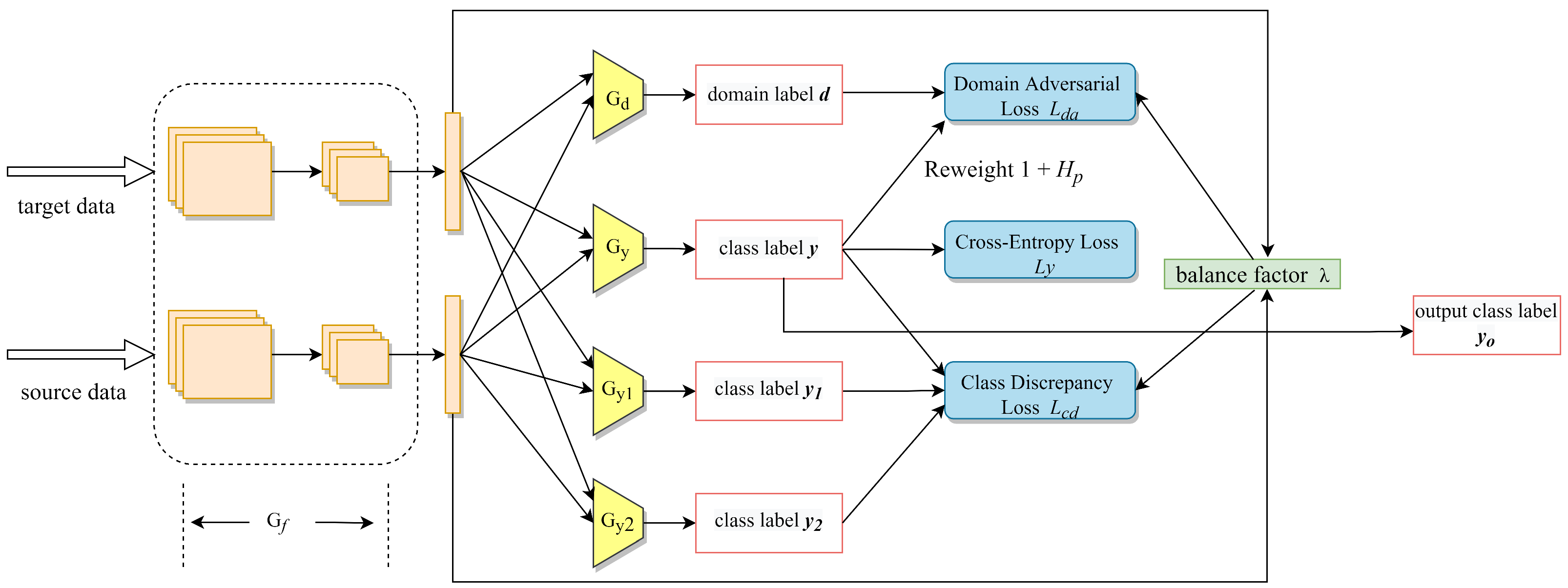
Original MCD and much derived research achieve this idea using two classifiers [46]. However, in the final step, several methods may be used for eventually classifying target samples. For example, several methods may use the best result between , . Several methods may combine two classifiers’ probability outputs and compare the sum to identify the final label. To remove such ambiguity, three classifiers are utilized, as shown in Figure 4, where is the main fault classifier; and are the two classifiers used only for computing discrepancy loss. Discrepancy loss contains three parts, and the equation below is our optimization objective:
where , , , are the feature generator and three fault classifiers that can be trained by the source domain data, respectively; , , , are their parameters; is the target domain sample that is input into the model. In our model, is used as the main classifier. Fixing and maximize the discrepancy between and in the target domain, and the target data excluded by the support of the source can be detected. Next, and are fixed and the discrepancy is minimized by training and to learn strong discriminating features.
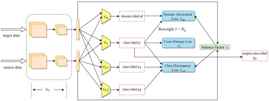
Figure 4.
The overall structure of proposed DRDA method. is feature generator, is domain discriminator, , and are three fault classifiers. d is the domain label generated by . y, and are class labels generated by , and , respectively.
3.2. Reweighted Adversarial Loss
In realistic domain adaptation scenarios, domain distributions that embody multi-mode structures prone to negative transfer are always a great challenge. Previous studies were aimed at finding excellent domain adaptation but rarely considered the role of each sample. They assumed that all the samples have equal transferabilities and make equal transfer contributions.
To promote positive transfer, it should be noticed that the transferability of each sample in the source domain or the target domain is different [47]. Different samples do not align well at the same time, that is, several samples with strong transferability may generate easily good transferable feature and have excellent performance in earlier iterations, whereas others may be just the opposite. Therefore, introducing an effective indicator to estimate such differences is needed. Inspired by information theory, entropy can measure uncertainty [48], and a reweighting strategy is proposed in this work to measure the degree of adaptation for each sample. The well-aligned samples obtain a lower entropy, whereas the poorly-aligned samples always have a higher entropy.
In the domain adaptation process, poorly aligned or slowly aligned samples should be given more attention. Hence, probability of a classifier is utilized to compute conditional entropy and reweight the domain adversarial loss of each sample. The traditional domain adversarial loss can be extended as follows:
where is the domain discriminator, and is its parameters. Joint with self-adaptive weight, domain adversarial loss can be rewritten as follows:
where is the weight of source sample and is the weight of target sample ; and are the probabilities for each class k towards and , respectively, computed by the main fault classifier ; and is the conditional information entropy. The larger of a sample means its worse adaptation performance in the current epoch of training. Therefore, its corresponding weight or in domain adversarial training will be larger. Through this mechanism of paying more attention to poorly aligned samples, the negative transfer caused by samples with poor transferability could be effectively eliminated.
3.3. Balance Factor for Domain Adaptation and Class Discrimination
In the former section, two main approaches are introduced to solve the domain adaptation problem. First, represented by a deep adversarial neural network (DANN), such methods aim to pursue feature representations that make both domains align well, and these common features can have a good transferability between domains. Second, similar to MCD, such methods believe that features aligning well are not sufficient, and obtaining excellent performance in the target domain task is the ultimate goal. For this purpose, these methods try to find class-specific features, and this process is so-called class discrimination.
Xiao et al. [44] proposed that the importance of two said items are different during algorithm iteration. For example, in the beginning of algorithm training, domain adaptation is more important than class discrimination. With an increase of training iterations, domain-share features are learned better and the class discrimination should receive more consideration. Inadequate and excessive domain adaptation or discriminant learning are harmful to positive transfer. Thus, how to balance these two items dynamically matters. It is well known that MMD is a good choice to measure the difference between two distributions. Naturally, MMD is used in this work as an estimator to observe the degree of adaptation between the two domains. MMD is defined as follows:
For class discrimination, based on linear discriminant analysis (LDA) [38] was proposed to estimate this item. LDA’s optimization objective of conventional two-category classification is defined as follows:
where is the intra-class scatter matrix, and is the inter-class scatter matrix [49]; indicates the mutual distance of clusters having different labels; and shows the compactness of data having the same labels. From this point, the class discrimination can be well measured. Expanding this idea to multiclass learning problem, the corresponding indicator is defined as follows:
The above discussion shows that MMD can depict the overall degree of domain adaptation. It can be applied in transfer learning, and the can be used to measure the feature’s degree of class discrimination. Combining these two items, a proper computation for balance factor can be found. However, it should be noticed that J(W) and MMD() may have different magnitudes, and normalization is necessary; and are defined as the corresponding normalized value:
where and are all located in interval [0,1]. The balance factor can be computed as follows:
Notably, is the weight of domain adaptation loss, and is the weight of class discrimination loss. Thus, the loss after adding the balance factor for domain adaptation and class discrimination is written as follows:
A smaller means better domain adaptation, and a larger indicates worse class discrimination. If domain adaptation is much better than class discrimination, the and can be very small and the corresponding is close to 0. If domain adaptation is much worse than class discrimination, the and will be close to 1 and approaches 1. If equals to 0.5, these two loss items have the same weight. The factor can dynamically adjust the weight of loss items and effectively control excessive or insufficient domain adaptation and class discrimination.
3.4. Dynamical Reweighted Domain Adaptation (DRDA)
The concrete architecture of the proposed DRDA model can be seen in Figure 4. According to the three parts, the overall optimization objective can be obtained:
The first item is classifier cross-entropy loss, the second item is reweighted adversarial loss (RAL), and the last item is class discrimination loss. The last two items multiply their own balance factor. Through the dynamic reweight for adversarial loss and balance factor to tune up the importance of domain adaptation and classifier training, our model effectively avoids negative transfer phenomenon and obtains a robust end-to-end cross domain bearing fault diagnosis system.
3.5. Training Steps
To obtain the optimal solution of the proposed model in the previous discussion, a feature generator, three fault classifiers, and one domain discriminator need to be trained. In the last subsection, the optimization objective was given, and how to solve this problem in four steps will be shown next. The expression is hyper parameters learning rate and in the experiments, 0.01 or 0.001 is selected; is the balance factor. The concrete computing method was given before, and only the detailed procedure of parameters updating will be discussed here.
Step A: The main fault classifier and feature generator are trained to make the main fault classifier more discriminantive and to classify the source data correctly. The network is trained to minimize the cross entropy loss and update the parameters, , :
Step B: Re-weighted domain adversarial loss is minimized. The feature generator is fixed, and only the domain adversarial module is trained. The parameters are updated as follows:
Step C: The feature generator is fixed, and three fault classifiers are trained to increase the discrepancy, which means minimizing . As MCD, the main fault classifier’s cross entropy loss is also added to . Parameters , , and are updated as follows:
Step D: Finally, the balanced reweighted domain adversarial loss and discrepancy loss are optimized. In this step, fault classifiers , , and domain adversarial module are fixed to update parameter :
4. Experiments
The advantage of the proposed DRDA is demonstrated through evaluation experiments on two cases: a bearing fault dataset from Case West Reserve University (CWRU) and a rotor test dataset (RT). Various previous cross-domain diagnosis models are introduced for a thorough comparison. The performance of the proposed method is compared with the following cross-domain bearing fault diagnosis methods in previous studies: CNN without domain adaptation, transfer component analysis (TCA), joint distribution analysis (JDA), deep adversarial neural networks (DANN), fine-grained adversarial network-based domain adaptation (FANDA), and maximum classifier discrepancy (MCD).
4.1. Cross-Location Diagnosis on CWRU Case
The bearing fault datasets from CWRU are available from its official website [50]. Bearings with faults are placed at either the fan end (FE) or the drive end (DE) in each test. The bearing types at the FE and DE are SKF 6203-2RS and SKF 6205-2RS, respectively. The parameters of the bearings at both ends are listed in Table 1.

Table 1.
Parameters of bearings in CWRU case.
The bearing data samples are divided into four classes according to health status: outer race fault (OF), inner race fault (IF), ball fault (BF), and health (H). These bearing faults are all obtained by artificial processing. The frequency of the sampling instrument is 12 kHz, and the depth of every fault is 0.007 inches. Specific working conditions corresponding to each dataset are shown in Table 2.

Table 2.
Description of experimental setting of CWRU case, which includes four categories and four domains.
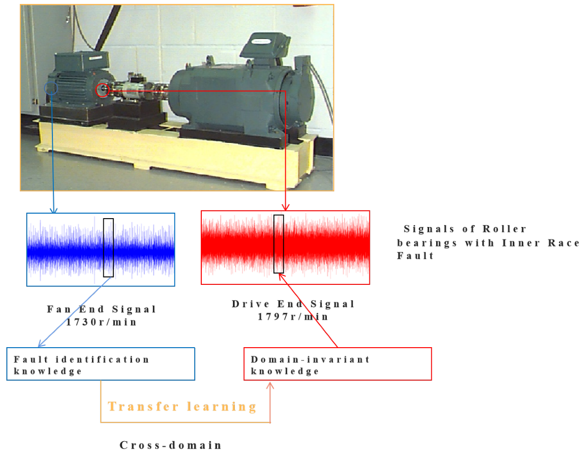
Data from and are collected from the bearing at the DE and their working loads are 0 HP (1797 r/min) and 3 HP (1730 r/min), respectively. Similarly, and are collected from the bearing at the FE and their working loads are also 0 HP (1797 r/min) and 3 HP (1730 r/min), respectively. Every dataset has 4000 examples, and the data shape of each time series example is . As shown in Figure 5 the CWRU case has four cross-location diagnosis tasks, i.e., →, →→, →. In each task, the former is the source domain with labels and the latter is the target domain without labels. The performance of each model is measured by the accuracy of fault predictions, which is defined as follows:
The diagnosis results of the four cross-location tasks are listed in Table 3. First, as expected, the performance of CNN is the worst among all the models because the distribution mismatch is not eliminated at all. The performance of CNN shows great difference in two reversed tasks, in which the source and target domains correspond to two identical datasets but the roles are reversed. For example, the diagnosis accuracy reached 69% in the task , but this number is reduced to approximately 44% in the corresponding reversed task , probably because of the large statistical distribution discrepancy between the two domains. This situation is clearly improved in other domain adaptation based models, and this confirms the necessity of domain adaptation in cross-domain bearing fault diagnosis.

Table 3.
Accuracy (%) of different models for CWRU case tasks.

Figure 5.
Cross-location bearing diagnosis tasks in CWRU case. Data samples with inner race faults are used for illustration.
Figure 5.
Cross-location bearing diagnosis tasks in CWRU case. Data samples with inner race faults are used for illustration.
Second, the mean accuracy of the proposed method in this paper is 89.38%, which outperforms that of all the comparison models. In addition, domain adaptation models that align both marginal and conditional data distribution of the two domains perform better than those that only align marginal distribution. The mean accuracy of FANDA and JDA exceeds 84%, whereas for the DANN aligning marginal distribution only, the mean accuracy is under 82%. The DANN utilizing adversarial domain adaptation performs better than TCA utilizing MMD criterion. Moreover, MCD performs better than TCA, JDA, and DANN due to the longer distance between the feature of each sample and the decision boundary, and it performs slightly worse than FANDA, probably because of an insufficient degree of domain adaptation.
The confusion matrices of task → shown in Figure 6 are introduced to analyze the results in more detail. The diagnosis accuracies of both FANDA and DANN are low, and the classifiers learned from them are unable to identify ball fault (BF) and outer race fault (OF) effectively. Part of the classification error of BF is corrected by MCD, whereas the misclassification phenomenon of OF is still evident. As can be seen from the figure, the proposed DRDA can accurately distinguish four kinds of bearing health status.
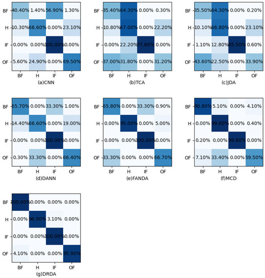
Figure 6.
Confusion matrices for the task → in CWRU case: (a) TCA, (b) JDA, (c) CNN, (d) DANN, (e) FANDA, (f) MCD, and (g) DRDA. The horizontal axis represents the predicted labels, and the vertical axis represents the true labels.
4.2. Cross-Speed Diagnosis on RT Case
Another dataset is collected from a rotor test in a practical scenario [51], and the schematic diagram of the test rig is shown in Figure 7. The power source of this rotor rig is a three-phase induction motor. The motor is connected to a shaft that is supported by a few bearings through a coupling. The bearings to be monitored are located at the right end of the shaft, and radial loads are provided by a loaded device. The vibration sensor for data collection is installed at point A. The bearing type in this diagnosis case is HRB 6010-2RZ (Harbin Bearing Manufacturing Co., Ltd., Harbin, China), and the related details are shown in Table 4.
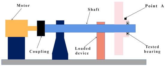
Figure 7.
The schematic diagram of the bearing test and sensor placement.

Table 4.
Parameters of tested bearings in RT case.
Similarly, data samples are divided into four classes according to health status: outer race fault (OF), inner race fault (IF), ball fault (BF), and health (H). Three kinds of faults are processed manually by wire electrical discharge machining. As shown in Figure 8, the rotational speed of the motor for domains C, D, and E is set to 3000, 5000, and 8000 revolutions per minute (rpm) during the measurement, respectively. Every domain has 4000 samples, and the data shape of each time series sample is . The frequency of the sampling instrument is 65,536 Hz, and the load exerted on the shaft and bearings by the radial loaded device is 2.0 kN. According to the said description, the details of RT case datasets are listed in the Table 5.
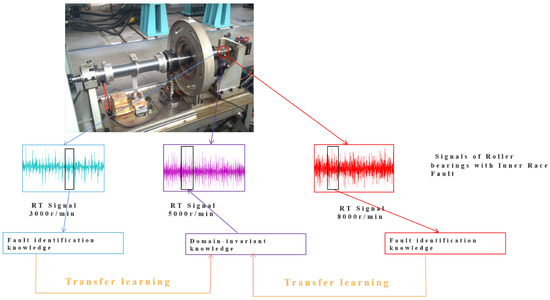
Figure 8.
Cross-speed bearing diagnosis tasks in RT case. Data samples with inner race faults are used for illustration.

Table 5.
Description of experimental setting on RT case, which includes four categories and three domains.
The designed RT case has six cross-domain diagnosis tasks in d, namely C→D, D→C, C→E, E→C, D→E, E→D, and their results are listed in Table 6.

Table 6.
Accuracy (%) of different models for RT case tasks.
Previous work in signal processing showed that the knowledge for fault diagnosis at variable speeds becomes more difficult to extract [52]. Moreover, the excellent performance of the proposed DRDA confirms that our model can robustly extract domain-invariant features under cross-speed diagnosis scenarios. First, as listed in Table 6, the performance of TCA and JDA degenerates more seriously than that of the other cross-domain diagnosis models. Their accuracies are under 30% in most cross-speed scenarios. For example, TCA and JDA only achieve an accuracy of 22.90% in the task of E→C. In accordance with the CWRU case, JDA performs slightly better than TCA in almost all tasks.
Second, the proposed DRDA performs better than other domain adaptation methods in almost all tasks, with a mean accuracy of 83.87% and an accuracy of 100% in tasks C→D, C→E, and D→E. Similarly, FANDA based on marginal and conditional distribution adaptation outperforms DANN in most tasks. In addition, the performances of almost all methods in tasks with a high speed dataset as the source domain and a low speed dataset as the target domain are unexpectedly much worse than those in reversed tasks (with a low speed dataset as the source domain and a high speed dataset as the target domain). For instance, the accuracies of FANDA, MCD, and DRDA are all above 95% in task C→E, whereas the numbers greatly reduce to approximately 50% in task E→C, because samples obtained under the working condition of high rotating speed have more noise, and extracting effective domain-invariant information for diagnosis is much more difficult when high speed datasets are set as the source domain.
To demonstrate the effectiveness of the proposed DRDA method more intuitively, the t-distributed stochastic neighbor embedding (t-SNE) technology [53] is utilized to visualize features by mapping them into 2D space. The t-SNE visual renderings of all the models on task D→C are shown in Figure 9. TCA and JDA almost fail completely on this difficult task in the RT case. CNN can only align a small part of the features with IF and OF. The confusion between IF and OF is serious in both DANN and FANDA. The confusion between IF and OF is remarkably improved in MCD, but the discrimination performance between H and BF deteriorates sharply. It is shown in Figure 9(g) that the distribution boundary of features from each class is tighter in DRDA, and the domain adaptation of features of samples with H, IF, and OF is clearly improved. In addition, another score metric is also introduced to verify the effect of the proposed DRDA method in eliminating negative transfer in difficult diagnosis tasks and improving the final diagnosis performance. The score is defined as
where precision is the proportion of bearing samples given the correct label to all bearing samples in the predicted class. Recall is the proportion of bearing samples given the correct label to all bearing samples in the real class. The score of four models that perform well under the accuracy metric in → and D→C tasks are shown in Table 7. As shown in the table, the diagnosis performance of the proposed DRDA method is still obviously improved compared with other three methods under the score metric. Moreover, compared with the traditional DANN and FANDA methods based on domain adversarial learning, the proposed DRDA has a greater improvement in diagnosis performance under the score metric than under the accuracy metric.
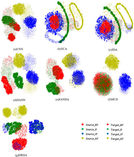
Figure 9.
The t-SNE features visualization of D→C task in RT case: (a) TCA features, (b) JDA features, (c) CNN features, (d) DANN features, (e) FANDA features, (f) MCD features, and (g) DRDA features.

Table 7.
score (%) of DANN, FANDA, MCD, and DRDA in → and D→C tasks.
4.3. Ablation Study
The effects of the RAL and balance factor for domain adaptation and class discrimination on enhancing the diagnosis accuracy are analyzed through comparative experiments. The performance of DRDA with or without RAL and balance factor on task E→C in the RT case is shown in Table 8. The diagnosis performance in this task is enhanced when RAL strategy and balance factor or one of them is introduced. Furthermore, our RAL strategy is introduced to the traditional DANN model. The performance of DANN with or without RAL module on task → in the CWRU case and task D→C in the RT case are shown in Figure 10, where great improvement can be noticed. This finding shows that the proposed RAL strategy can also promote positive transfer when used in other domain adaptation methods based on adversarial training.

Table 8.
Accuracy (%) of DRDA with or without RAL and balance factor on task E → C in the RT case.
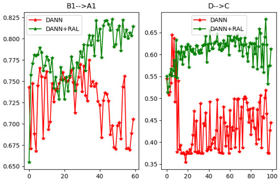
Figure 10.
The performance of DANN and DANN with RAL on → task in the CWRU case and D→C task in RT case. The horizontal axis represents the training epochs, and the vertical axis represents the diagnosis accuracy.
5. Conclusions
A novel domain adaptation method named DRDA for cross-domain bearing fault is proposed in this paper. The negative transfer caused by samples with poor transferability in cross-domain bearing fault diagnosis is eliminated in DRDA by introducing a reweighted adversarial loss strategy. The negative transfer caused by the imbalance between the classifier training and the domain adaptation in cross-domain bearing fault diagnosis is eliminated in the proposed method by constructing a powerful balance factor . The performance of the DRDA measured by accuracy and score are better than other comparison methods in cross-location and cross-speed diagnosis tasks, as can be seen from Table 3, Table 6 and Table 7. After eliminating the negative transfer caused by the imbalance between the classifier training and domain adaptation, the percentage of samples correctly classified by the DRDA method in each class has been improved, as can be seen from the confusion matrix in Figure 6. The improvement of the DRDA in terms of marginal alignment and conditional distribution alignment after eliminating the negative transfer caused by samples with poor transferability is shown in the t-SNE features visualization of Figure 9. In addition, the ablation study shows that the two modules proposed in this article can still improve the diagnosis performance by eliminating negative transfer when they are introduced into the diagnosis model separately. To sum up, sufficient comparative experiments prove the feasibility and the superiority of the proposed novel domain adaptation method for cross-domain bearing fault diagnosis.
Author Contributions
Y.M.: conceptualization, methodology, software, writing—original draft, investigation, funding acquisition. J.X. Data curation, Writing—review editing, Validation, Investigation, Funding acquisition. L.X.: software, methodology. J.L.: software, visualization. All authors have read and agreed to the published version of the manuscript.
Funding
This research is supported by the National Key R&D Program of China (Grant No. 2020YFB2007700) and the National Natural Science Foundation of China (Grant No. 52175094).
Institutional Review Board Statement
Not applicable.
Informed Consent Statement
Not applicable.
Acknowledgments
This research is supported by the National Key R and D Program of China (Grant No. 2020YFB2007700) and the National Natural Science Foundation of China (Grant No. 52175094).
Conflicts of Interest
The authors declare that they have no known competing financial interest or personal relationships that could have appeared to influence the work reported in this paper.
References
- Xu, Z.; Mei, X.; Wang, X.; Yue, M.; Jin, J.; Yang, Y.; Li, C. Fault diagnosis of wind turbine bearing using a multi-scale convolutional neural network with bidirectional long short term memory and weighted majority voting for multi-sensors. Renew. Energy 2022, 182, 615–626. [Google Scholar] [CrossRef]
- He, Z.; Shao, H.; Wang, P.; Lin, J.; Yang, Y. Deep transfer multi-wavelet auto-encoder for intelligent fault diagnosis of gearbox with few target training samples. Knowledge-Based Systems. Deep transfer multi-wavelet auto-encoder for intelligent fault diagnosis of gearbox with few target training samples. Knowl.-Based Syst. 2019, 191, 105313. [Google Scholar]
- Shao, H.; Ding, Z.A.; Cheng, J.A.; Jiang, H.C. Intelligent fault diagnosis among different rotating machines using novel stacked transfer auto-encoder optimized by PSO. ISA Trans. 2020, 105, 308–319. [Google Scholar]
- Han, B.; Zhang, X.; Wang, J.; An, Z.; Zhang, G. Hybrid distance-guided adversarial network for intelligent fault diagnosis under different working conditions. Measurement 2021, 176, 109197. [Google Scholar] [CrossRef]
- Xue, F.; Zhang, W.; Xue, F.; Li, D.; Fleischer, J. A novel intelligent fault diagnosis method of rolling bearing based on two-stream feature fusion convolutional neural network. Measurement 2021, 176, 109226. [Google Scholar] [CrossRef]
- Ur Rehman, M.H.; Yaqoob, I.; Salah, K.; Imran, M.; Jayaraman, P.P.; Perera, C. The role of big data analytics in industrial Internet of Things. Future Gener. Comput. Syst. 2019, 99, 247–259. [Google Scholar] [CrossRef] [Green Version]
- Li, J.; Yao, X.; Wang, H.; Zhang, J. Periodic impulses extraction based on improved adaptive vmd and sparse code shrinkage denoising and its application in rotating machinery fault diagnosis. Mech. Syst. Signal Process. 2019, 126, 568–589. [Google Scholar] [CrossRef]
- Yan, X.; Dda, B.; Jy, C. Multi-fault diagnosis of rotating machinery based on deep convolution neural network and support vector machine. Measurement 2020, 156, 107571. [Google Scholar]
- Chen, G.; Liu, M.; Chen, J. Frequency-temporal-logic-based bearing fault diagnosis and fault interpretation using Bayesian optimization with Bayesian neural networks. Mech. Syst. Signal Process. 2020, 145, 106951. [Google Scholar] [CrossRef]
- Tang, L.; Xuan, J.; Shi, T.; Zhang, Q. Envelopenet: A robust convolutional neural network with optimal kernels for intelligent fault diagnosis of rolling bearings. Measurement 2021, 180, 109563. [Google Scholar] [CrossRef]
- Soualhi, A.; Medjaher, K.; Zerhouni, N. Bearing Health Monitoring Based on Hilbert-Huang Transform, Support Vector Machine, and Regression. IEEE Trans. Instrum. Meas. 2015, 64, 52–62. [Google Scholar] [CrossRef] [Green Version]
- He, G.; Ding, K.; Lin, H. Fault feature extraction of rolling element bearings using sparse representation. J. Sound Vib. 2016, 366, 514–527. [Google Scholar] [CrossRef]
- Lu, S.; Wang, X.; He, Q.; Liu, F.; Liu, Y. Fault diagnosis of motor bearing with speed fluctuation via angular resampling of transient sound signals. J. Sound Vib. 2016, 385, 16–32. [Google Scholar] [CrossRef]
- Zhou, P.; Lu, S.; Liu, F.; Liu, Y.; Li, G.; Zhao, J. Novel synthetic index-based adaptive stochastic resonance method and its application in bearing fault diagnosis. J. Sound Vib. 2017, 391, 194–210. [Google Scholar] [CrossRef]
- Feng, K.; Smith, W.A.; Borghesani, P.; Randall, R.B.; Peng, Z. Use of cyclostationary properties of vibration signals to identify gear wear mechanisms and track wear evolution. Mech. Syst. Signal Process. 2020, 150, 107258. [Google Scholar] [CrossRef]
- Peeters, C.; Antoni, J.; Helsen, J. Blind filters based on envelope spectrum sparsity indicators for bearing and gear vibration-based condition monitoring. Mech. Syst. Signal Process. 2020, 138, 106556.1–106556.17. [Google Scholar] [CrossRef]
- Shao, H.; Jiang, H.; Zhang, H.; Duan, W.; Liang, T.; Wu, S. Rolling bearing fault feature learning using improved convolutional deep belief network with compressed sensing. Mech. Syst. Signal Process. 2018, 100, 743–765. [Google Scholar] [CrossRef]
- Su, G.; Fang, D.; Chen, J.; Rui, Z. Sensor Multifault Diagnosis With Improved Support Vector Machines. IEEE Trans. Autom. Sci. Eng. 2015, 14, 1053–1063. [Google Scholar]
- Gao, X.; Hou, J. An improved SVM integrated GS-PCA fault diagnosis approach of Tennessee Eastman process. Neurocomputing 2016, 174, 906–911. [Google Scholar] [CrossRef]
- Gao, F.; Zhao, C. A Nested-loop Fisher Discriminant Analysis Algorithm. Chemom. Intell. Lab. Syst. 2015, 146, 396–406. [Google Scholar]
- Zhang, Q.; Tang, L.; Sun, M.; Xuan, J.; Shi, T. A statistical distribution recalibration method of soft labels to improve domain adaptation for cross-location and cross-machine fault diagnosis. Measurement 2021, 182, 109754. [Google Scholar] [CrossRef]
- Witten, I.H.; Frank, E.; Hall, M.A. Chapter 6—Implementations: Real Machine Learning Schemes; Elsevier Inc.: Amsterdam, The Netherlands, 2011. [Google Scholar]
- Lei, Y.; Li, N.; Guo, L.; Li, N.; Yan, T.; Jing, L. Machinery health prognostics: A systematic review from data acquisition to RUL prediction. Mech. Syst. Signal Process. 2018, 104, 799–834. [Google Scholar] [CrossRef]
- Zheng, H.; Wang, R.; Yang, Y.; Li, Y.; Xu, M. Intelligent Fault Identification Based on Multisource Domain Generalization Towards Actual Diagnosis Scenario. IEEE Trans. Ind. Electron. 2019, 67, 1293–1304. [Google Scholar] [CrossRef]
- Wu, Z.; Jiang, H.; Lu, T.; Zhao, K. A deep transfer maximum classifier discrepancy method for rolling bearing fault diagnosis under few labeled data. Knowl.-Based Syst. 2020, 196, 105814. [Google Scholar] [CrossRef]
- Si, J.; Shi, H.; Chen, J.; Zheng, C. Unsupervised deep transfer learning with moment matching: A new intelligent fault diagnosis approach for bearings. Measurement 2020, 172, 108827. [Google Scholar] [CrossRef]
- Wang, X.; Ren, J.; Liu, S. Distribution Adaptation and Manifold Alignment for Complex Processes Fault Diagnosis. Knowl.-Based Syst. 2018, 156, 100–112. [Google Scholar] [CrossRef]
- Wang, J.; Xie, J.; Zhang, L.; Duan, L. A factor analysis based transfer learning method for gearbox diagnosis under various operating conditions. In Proceedings of the 2016 IEEE International Symposium on Flexible Automation (ISFA), Cleveland, OH, USA, 1–3 August 2016. [Google Scholar]
- Li, X.; Zhang, W.; Ding, Q.; Sun, J.Q. Multi-Layer domain adaptation method for rolling bearing fault diagnosis. Signal Process. 2019, 157, 180–197. [Google Scholar] [CrossRef] [Green Version]
- Xie, J.; Zhang, L.; Duan, L.; Wang, J. On cross-domain feature fusion in gearbox fault diagnosis under various operating conditions based on Transfer Component Analysis. In Proceedings of the 2016 IEEE International Conference on Prognostics and Health Management (ICPHM), Ottawa, ON, Canada, 20–22 June 2016. [Google Scholar]
- Goodfellow, I.; Pouget-Abadie, J.; Mirza, M.; Xu, B.; Warde-Farley, D.; Ozair, S.; Courville, A.; Bengio, Y. Generative Adversarial Networks. Adv. Neural Inf. Process. Syst. 2014, 3, 2672–2680. [Google Scholar] [CrossRef]
- Li, X.; Zhang, W.; Ma, H.; Luo, Z.; Li, X. Deep learning-based adversarial multi-classifier optimization for cross-domain machinery fault diagnostics. J. Manuf. Syst. 2020, 55, 334–347. [Google Scholar] [CrossRef]
- Qian, W.; Li, S.; Jiang, X. Deep transfer network for rotating machine fault analysis. Pattern Recognit. 2019, 96, 106993. [Google Scholar] [CrossRef]
- Zhang, B.; Li, W.; Tong, Z.; Zhang, M. Bearing fault diagnosis under varying working condition based on domain adaptation. In Proceedings of the 25th International Congress on Sound and Vibration (ICSV25), London, UK, 23–27 July 2017. [Google Scholar]
- Wu, Z.; Jiang, H.; Zhao, K.; Li, X. An adaptive deep transfer learning method for bearing fault diagnosis. Measurement 2019, 151, 107227. [Google Scholar] [CrossRef]
- Yu, K.; Fu, Q.; Ma, H.; Lin, T.R.; Li, X. Simulation data driven weakly supervised adversarial domain adaptation approach for intelligent cross-machine fault diagnosis. Struct. Health Monit. 2020, 20, 2182–2198. [Google Scholar] [CrossRef]
- Saito, K.; Watanabe, K.; Ushiku, Y.; Harada, T. Maximum Classifier Discrepancy for Unsupervised Domain Adaptation. In Proceedings of the 2018 IEEE/CVF Conference on Computer Vision and Pattern Recognition, Salt Lake City, UT, USA, 18–22 June 2018. [Google Scholar]
- Shuang, L.; Shiji, S.; Gao, H.; Zhengming, D.; Cheng, W. Domain Invariant and Class Discriminative Feature Learning for Visual Domain Adaptation. IEEE Trans. Image Process 2018, 27, 4260–4273. [Google Scholar]
- Yu, C.; Wang, J.; Chen, Y.; Huang, M. Transfer Learning with Dynamic Adversarial Adaptation Network. In Proceedings of the 2019 IEEE International Conference on Data Mining (ICDM), Beijing, China, 8–11 November 2019. [Google Scholar]
- Pan, S.J.; Qiang, Y. A Survey on Transfer Learning. IEEE Trans. Knowl. Data Eng. 2010, 22, 1345–1359. [Google Scholar] [CrossRef]
- Ge, L.; Gao, J.; Ngo, H.; Li, K.; Zhang, A. On handling negative transfer and imbalanced distributions in multiple source transfer learning. Stat. Anal. Data Min. 2014, 7, 254–271. [Google Scholar] [CrossRef]
- Martini, A.; Troncossi, M.; Vincenzi, N. Structural and Elastodynamic Analysis of Rotary Transfer Machines by Finite Element Model. J. Serbian Soc. Comput. Mech. 2017, 11, 1–16. [Google Scholar] [CrossRef] [Green Version]
- Cocconcelli, M.; Troncossi, M.; Mucchi, E.; Agazzi, A.; Rivola, A.; Rubini, R.; Dalpiaz, G. Numerical and Experimental Dynamic Analysis of IC Engine Test Beds Equipped with Highly Flexible Couplings. Shock Vib. 2017, 2017, 5802702. [Google Scholar] [CrossRef] [Green Version]
- Xiao, N.; Zhang, L. Dynamic Weighted Learning for Unsupervised Domain Adaptation. In Proceedings of the IEEE/CVF Conference on Computer Vision and Pattern Recognition, Nashville, TN, USA, 20–25 June 2021. [Google Scholar]
- Zhang, Y.; Zhang, Y.; Wang, Y.; Qi, T. Domain-Invariant Adversarial Learning for Unsupervised Domain Adaption. arXiv 2018, arXiv:1811.12751. [Google Scholar]
- Jiao, J.; Zhao, M.; Lin, J. Unsupervised Adversarial Adaptation Network for Intelligent Fault Diagnosis. IEEE Trans. Ind. Electron. 2019, 67, 9904–9913. [Google Scholar] [CrossRef]
- Shu, Y.; Cao, Z.; Long, M.; Wang, J. Transferable Curriculum for Weakly-Supervised Domain Adaptation. In Proceedings of the AAAI Conference on Artificial Intelligence, Honolulu, HI, USA, 27 January 2019; Volume 33, pp. 4951–4958. [Google Scholar]
- Núñez, J.A.; Cincotta, P.M.; Wachlin, F.C. Information entropy. Celestial Mech. Dyn. Astr. 1996, 64, 43–53. [Google Scholar] [CrossRef]
- Chen, X.; Wang, S.; Long, M.; Wang, J. Transferabi1ity vs. discriminabi1ity batch spectra1 pena1ization for adversaria1 domain adaptation. In Proceedings of the 36th International Conference on Machine Learning, Long Beach, CA, USA, 9–15 June 2019. [Google Scholar]
- Smith, W.A.; Randall, R.B. Rolling element bearing diagnostics using the Case Western Reserve University data: A benchmark study. Mech. Syst. Signal Process. 2015, 64–65, 100–131. [Google Scholar] [CrossRef]
- Duan, J.; Shi, T.; Zhou, H.; Xuan, J.; Zhang, Y. Multiband Envelope Spectra Extraction for Fault Diagnosis of Rolling Element Bearings. Sensors 2018, 18, 1466. [Google Scholar] [CrossRef] [PubMed] [Green Version]
- Wang, Y.; Xu, G.; Zhang, Q.; Liu, D.; Jiang, K. Rotating speed isolation and its application to rolling element bearing fault diagnosis under large speed variation conditions. J. Sound Vib. 2015, 348, 381–396. [Google Scholar] [CrossRef]
- Van der Maaten, L.; Hinton, G. Visualizing data using t-SNE. J. Mach. Learn. Res. 2008, 9, 2579–2605. [Google Scholar]
Publisher’s Note: MDPI stays neutral with regard to jurisdictional claims in published maps and institutional affiliations. |
© 2022 by the authors. Licensee MDPI, Basel, Switzerland. This article is an open access article distributed under the terms and conditions of the Creative Commons Attribution (CC BY) license (https://creativecommons.org/licenses/by/4.0/).


