Abstract
Weeds compete with crops for water, nutrients, and light consequently, have adverse effects on the crop yield and overall productivity. Mechanical weeding is the most common non-chemical method for weed control, which is applied in organic farming, and the weed cultivator is the most common implement in mechanical weeding. This study aimed to design and develop an innovative active tool to optimize the cultivation depth, which can avoid damage to crop roots and improve the key performance indicators of an inter-row cultivator. A quasi-Newton optimization method and a hybrid of the non-dominated sorting genetic algorithm (NSGA-II) and goal attainment method were separately applied to synthesize and develop a four-bar mechanism for weeding requirements. The transmission angle of the mechanism and the desired path of the weeding blade were simultaneously optimized using these multi-objective optimization techniques. The performance of the developed four-bar cultivator based on the optimization techniques was compared with the ones developed based on the classic methods and also with several conventional tools evaluated in other studies. The results showed that applying the quasi-Newton optimization method and hybrid genetic algorithm can propose a more effective weed cultivator in terms of performance indicators, namely weeding performance, mechanical damage to crop plants and cultivation depth. In addition, the optimization of the transmission angle guaranteed the smooth rotations in the mechanism’s joints.
1. Introduction
In smart farming, the presence of weeds is one of the major problems that contribute to yield losses in terms of the agricultural production level, and they should be removed [1,2]. Overall, weeds are more harmful than other biotic factors, such as animal pests and pathogens, and have the potential to reduce the crop yield up to 34%, while this quantity is 18% and 16% for animal pests and pathogens, respectively [3,4].
Different methods for weed management have been developed, including chemical and mechanical control. Nowadays, the interest in organic and low-input farming systems has shifted focus away from chemical control onto other alternative methods [5,6]. Chemical control is efficient but has serious environmental impacts [5,7,8], including water contamination [9] and widespread development of herbicide-resistant weeds [5,7]. As a result, most countries have limited the use of herbicides. For instance, the EU passed regulations to limit the use of pesticides in 2009, and most of these products have been removed from the European market [10,11]. On the other hand, although effective, hand weeding is laborious, time-consuming and costly [12,13], and it can only be applied to expensive products, such as strawberries [14,15]. Therefore, it is necessary to fill the gap of chemical control by other reliable methods, such as mechanical control using weed cultivators. In the past two decades, extensive research on these types of methods has been carried out [10,11].
The inter-row cultivator is an implement designed for mechanical weed control between the crop rows, whereas the intra-row cultivator is the one used for the weed control of small areas between crop plants on each crop row. Although intra-row weeding is a more serious challenge to contend with [16], inter-row cultivators suffer from a number of shortcomings [17,18]. There are several types of inter-row cultivators, among which the harrow, used for both inter-row and intra-row weeding, is the most commonly used one in Europe [17,19]. This weeder consists of a variety of rigid or flexible tines used for weeding operation. However, the performance of this type is less effective than the other types used for inter-row weeding [17], which is rooted in various factors, among which a heavy dependence on depth wheels is of utmost importance. In other words, variations in soil moisture content and bulk density can lead to variations in working depth and cause damage to the crop roots [20]. Dependence on depth wheels is an issue not only for harrows but also for the other types that are pulled rather than mounted on a tractor [20]. Rotary hoe is another common cultivator that is a ground driven type. The machine consists of some hoe wheels mounted on horizontal axles. Each hoe wheel has several curved teeth acting as a weeder. Although that is widely used in North America, it is less able to control the established weeds, specifically at high speeds, since fast speed can lead to a decrease in teeth penetration [17,19,21]. Brush weeder is an active implement that is suitable for near-row weeding. The machine consists of horizontal-axis or vertical-axis nylon or fiberglass brushes acting as a weeder. Nevertheless, it does not do as well as other common types and causes dust problems in dry conditions [17]. Sweep is another type that is used worldwide [22]. This implement has some shanks mounted on a frame and each shank has a blade cutting weeds’ roots below the surface. This type is the most suitable one for high-speed operation [17]. Nonetheless, it uses passive tools. An important problem associated with such tools is their low power efficiency due to the fact that they are pulled by the tractor, which leads to wasting a large amount of energy through the drawbar of the tractor, whereas active tools directly transmit a considerable amount of energy, generated by the engine, into the soil as they are driven by a PTO shaft [23,24]. Moreover, there is a risk of crop root damaging while this implement is working too deep and too close to crop rows [19,22]. Ducksfoot, which usually has several curved shanks attached to some blades and is generally fitted to a spring tine, is another passive type that is more aggressive than the sweep and is suitable for inter-row weed management. Nevertheless, vigorous soil movement would pose problems in narrow rows and bury young crop plants [17]. The weeding depth of cultivators should be over 30 mm and should not exceed 40 mm [19,25]. Accordingly, in order for cultivators to curb their depth of penetration, conditions such as a considerable planting depth and dry surface soil should be available [14]. On the other hand, the increased working depth cannot significantly increase weed removal; however, it increases soil disturbance [8]. Besides weed control, soil disturbance is another performance indicator for cultivators as a very small amount of soil should be turned over during the operation due to the fact that severe disturbance may damage the crops [8]. Against this background and considering the environmental impacts of herbicides, this study aimed to design and develop an efficient and simple active implement for weed control.
The study further focuses on the design of two four-bar path-generator mechanisms using two different optimization methods with regard to the above-mentioned weeding requirements considering the constraints governing the problem. The four-bar mechanism was selected due to its simple development, assembly and maintenance besides its satisfactory accuracy [26,27,28]. In fact, the cultivator design problem can be viewed as an optimal path generation problem for a four-bar mechanism. The design baseline is a multi-objective optimal design, an area of mathematical optimization involving more than one objective function to be optimized simultaneously. The genetic algorithm (GA), as a highly popular evolutionary algorithm having well-tried records in agricultural engineering [29,30,31,32], is employed and hybridized with a goal attainment method in the synthesis of the first mechanism, whereas a quasi-Newton optimization method (QNM) is used for the second mechanism synthesis. The results from both optimal design methods are compared with each other and with those of other studies, and then the two mechanisms are simulated statically and dynamically to verify the results. Finally, the optimal mechanism is developed for in situ experimentation.
The following portions of this paper are organized as follows: Section 2 discusses the related literature on four-bar mechanisms designed for mechanical weeding. Section 3 identifies the operationally suitable four-bar mechanism for the weeding requirements. Section 4 describes the optimal design process in terms of the objective functions, the constraints of the problem and the optimization methods. Section 5 outlines the experimental study. Section 6 presents the main results of the study and explores the significance of the results. The conclusions of the study are given in Section 7.
2. Literature Review
2.1. Four-Bar Mechanism
The four-bar mechanism is one of the well-established mechanisms for path synthesis in the past few decades. In the path synthesis of four-bar mechanisms, independent design parameters (e.g., mechanism dimensions, coordinates of the base pin and linkage angles) should be determined to allow a specific point on the coupler link of the mechanism to track a predefined path. The methods used in the literature on this mechanism can be divided into three categories: analytical, graphical and numerical. The analytical methods are accurate but have limited precision points [27,33,34,35,36]. The graphical methods are fast and simple with low accuracy [27,33]. Several numerical methods have been used for four-bar mechanism synthesis in the past [27,37,38]. In all of these methods, one or more objective functions are defined using the design variables. The objective function(s) is (are) then optimized following the introduction of a number of potential constraints. These methods have overcome the limited-precision-point problem provided that a sensible tolerance between the tracked path by the mechanism and the desired path could be accepted. There is a chance of convergence towards a local optimum instead of a global one during the search process over the search space, so evolutionary algorithms were developed to address this problem. They are inspired by Darwinism and, unlike classical numerical methods, a set of points—instead of one point—search the design space, improving the chance of reaching the global optimum. Additionally, they are easy to implement with low computational costs as they require no in-depth knowledge of the search space and the mathematical characteristics of the objective function (e.g., gradient) [26,33,35,36].
2.2. Four-Bar Mechanism for Weeding
Four-bar mechanisms have been successfully studied in different areas of agricultural machinery [28,39,40,41]. Moreover, four-bar linkage is a well-established mechanism in the path generation of tillage tools under the soil surface [24,42,43,44,45,46]. Using a four-bar mechanism for weeding could improve some performance indicators of cultivators, such as optimal working depth and soil disturbance [14,25,47]. Nevertheless, there are only a few papers on designing or evaluating four-bar mechanisms for weeding, and there is a lack of studies on this topic [14,25,47]; furthermore, there is no study on the optimal design of mechanical weeders.
As regards the weeding requirements described in Section 1, the hand motion of farmers during the manual removal of weeds was the source of inspiration for designing and evaluating a cultivator [14,25]. A four-bar mechanism was employed in these studies to imitate this motion. The literature suggests a 100 mm efficient motion stroke. However, in this study, the hand motions of three farmers were surveyed by a steel ruler and a piece of string to define more precise values, and the final value is the arithmetic mean calculated from a set of 30 numbers. All 30 values were in the 90 mm to 120 mm range. Figure 1 shows the approximate path of a hoe operated by a farmer’s hand. As shown, the efficient motion stroke is 102.5 mm and working depth is 40 mm. The main idea of this approach is to track the path shown in Figure 1 by a weeding blade.
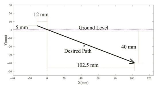
Figure 1.
The desired path for a coupler point of the four-bar mechanism.
Although the idea of imitating the hand motion of farmers for weeding was a brilliant idea, the proposed mechanisms in such papers were far from the design expectations. To illustrate, the authors of ref. [14] employed a path generation method for a weeding blade, which was limited to three precision points, the points located on the desired path, because of the analytical–graphical approach of the research. As a result, the synthesized path was very different from the desired path. The other shortcoming of the research was that the path was generated for a stationary mechanism, in the first place, and the travel velocity was introduced to the problem after the mechanism synthesis. It is obvious that this approach exacerbated the above-said error—the mismatch between the desired and generated path. Other researchers [25] employed a four-bar mechanism having been developed by Rural Development Administration of Republic of Korea (RDA). Although there is not enough information about the path generation method of the mechanism, the authors of that paper discussed the drawbacks of the mechanism by means of simulation software. The dynamic simulation revealed that the synthesized path of the mechanism was far from the desired one, and such a mismatch is attributable to a wrong design method [25]. Both above-mentioned mechanisms have other serious drawbacks as they were designed without the inclusion of a transmission angle through the design process, which would lead to two different impractical mechanisms. The transmission angle is an indicator of energy and torque transmission [26,36,48]. By minimizing the deviation of this angle from right angle (90 degrees), the mechanism moves smoothly, curbing excessive wear in its joints, and the power required for rotating the mechanism can be as small as possible [26]. Another disadvantage of these mechanisms is associated with the effective stroke of the weeding blade during weeding operation, which is an indicator of the interaction time between soil and weeding blade during a weeding cycle. As discussed in Section 6, both above-mentioned mechanisms have inappropriate effective stroke.
As far as the above-mentioned shortcomings are concerned, it is necessary to design a mechanism capable of tracking the sufficient number of precision points on the desired path and synthesize a reasonable transmission angle to ensure suitable energy and torque transmission. Moreover, the mechanism’s blade must have enough interaction time through the soil. What is more, the mechanism must be synthesized dynamically, not statically, and the forward speed of the mechanism should be considered in the design process.
3. Operational Requirements
Based on Section 1 and Section 2, an operationally suitable four-bar cultivator may materialize as follows:
- (1)
- The weeding blade of cultivator (the coupler point of four-bar mechanism) should be capable of tracking the path shown in Figure 1 while the cultivator is operating in the field.
- (2)
- The mechanism’s transmission angle should not deviate more than 50 degrees from right angle (90 degrees) during a full rotation of input link [49,50].
- (3)
- The proposed mechanism should have a reasonable size considering its in-field application.
In order to meet the first two items, in the first place, it is necessary to include the travel velocity of the cultivator in the path synthesis problem. This is realized through the displacement and velocity vector analysis in Section 4.1. That is, this study synthesizes the mechanism dynamically rather than statically. In the second place, the design approach overcomes precision point limitations using HGA and QNM. As a consequence, better results can be achieved by using a sufficient number of precision points on the desired path. To put it another way, using HGA and QNM and a sufficient number of precision points, a targeted path rather than an indiscriminate one having been previously tracked by conventional tools is defined and synthesized. Finally, the transmission angle will be optimized during the design process. To sum up, following the inclusion of travel velocity to the problem, the simultaneous optimization of the tracking error and transmission angle are considered in this study. Note that these two objectives are inconsistent, i.e., improvement in one exacerbates the other and vice versa. In addition, due to the mechanism’s in-field application and also manufacturing process, the design method must fulfill the third item. It is obtained by imposing bounds to the design variables related to the mechanism’s size.
4. Theoretical Framework
4.1. The Path Identification of Weeding Blade
Since the cultivator is rear-mounted on the tractor, it is inevitable to introduce the tractor travel velocity to the problem of weeding blade path identification. Following the inclusion of this parameter, the desired path for the weeding blade was determined through displacement and velocity vector analysis, which is inspired by the method presented by Hettiaratchi [42]. In other words, this vector analysis neutralizes the adverse effect of the tractor motion on the synthesis process.
The path shown in Figure 1 is the one that the coupler point of the four-bar mechanism should track. Finally, the weeding blade is attached to the coupler point. This motion—i.e., blade traveling from the surface into soil depth—is referred to as the absolute motion of the weeding blade, and its respective displacement vector is B (the path tracked with respect to ground reference). This is the absolute displacement vector of the blade and is measured from the perspective of a bystander. It should be noted that the tractor travels at a constant speed during the weeding operation. T is the displacement vector of the tractor. If the relative displacement vector of the blade to the tractor is designated with R (the path tracked with respect to the tractor reference), the desired displacement, B, can be defined by Equation (1).
Figure 2a is the vector representation of this equation. Note that, in this figure, the weeding blade travels at its effective 102.5 mm stroke and penetrates 40 mm. In its passive stroke, the blade travels 5 mm above the surface and has a 12 mm longitudinal stroke.
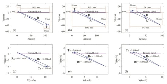
Figure 2.
(a–c) Displacement vector diagrams; (d–f) velocity vector diagrams for motion of tractor (T) and weeding blade (R, B).
As shown, Figure 2a presents the penetration stroke of the weeding blade into the soil. It is now ideal for the blade to be pulled back from the soil through the same path it penetrated (Figure 2b). Although this is an optimal situation, it makes the mechanism design quite difficult. This is explained in Figure 2d,e. They display the mean linear velocity vectors corresponding to Figure 2a,b, respectively. The tractor travel speed is considered 2 km h−1 for the weeding operation. It is clear that the magnitude of vector should remain constant if the blade is to return again via its penetration path, and only its direction should be reversed. As the tractor travel velocity vector, , is also constant, the mean linear velocity vector of the weeding blade relative to the tractor (relative velocity vector ) should change. Since the four-bar mechanism is powered by the tractor power take-off shaft (PTO), the fact that the input link of the mechanism can have two different speeds, within a rotation, is impossible. Therefore, it is inevitable to assume constant values for and vectors (Figure 2d,f) and only accept variable values for . Figure 2c shows the displacement vectors equivalent to Figure 2f. From Figure 2a,c, it can be found that the T vector with a smaller magnitude means smaller deviation of the B vector through the return path.
Based on the above discussion, the precise path of the weeding blade motion relative to the tractor can be drawn as shown in Figure 3. The points on the path are the precision points that the mechanism should track. The coordinates of these points are listed in Table 1. It is obvious that the path shown in Figure 3 is the desired one for the mechanism in the tractor’s stationary state, and it will be transformed into Figure 1 after the tractor begins to travel in the field.
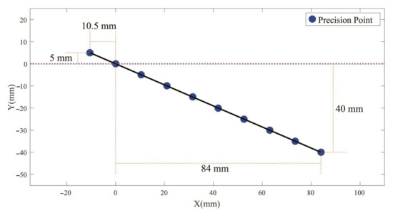
Figure 3.
Precise path of the weeding blade’s motion relative to the tractor.

Table 1.
Coordinates of precision points.
It can be concluded that the ratio—i.e., the tractor travel velocity to mean linear velocity of the weeding blade relative to the tractor—should be constant during the weeding operation (). To this end, since the four-bar mechanism is driven by PTO during the weeding operation and is dependent on the rotational speed of PTO, the tractor PTO should be set in the transmission driven mode. In this case, the tractor throttle will be set to a fixed value, and the forward speed must be changed by shifting gears during the operation in order for the rotational speed of PTO to increase in proportion to the forward speed of tractor. Any change in the forward speed will translate into a change in the rotational speed of PTO, and the ratio of the tractor forward speed to mean linear speed of the weeding blade, which is mounted at the coupler point of the mechanism, will remain constant. In general, the forward speed is recommended to be constant for the weeding operation. However, due to the special geology of the fields and the ground unevenness, it is possible that this ratio varies during weeding operation. Therefore, in Section 6.5 and Section 6.6, the behavior of the cultivator at different speed ratios was studied to ensure the capability of designed mechanism for other real-life scenarios.
A deeper review of Figure 3 and the coordinates of precision points in Table 1 shows a need for a mechanism capable of tracking this path at penetration and return strokes. As can be known, there are plenty of pin-jointed mechanisms generating an approximate or exact straight-line motion. The better-known ones are Watt, Roberts, Chebyschev, Evans, Hart inversor and Peaucellier straight-line linkages. However, there is no simple crank–rocker type among these linkages, so they cannot be used with the continuous rotation of tractor PTO [51]. Moreover, their coupler points generate a straight line in a part of their input links’ rotation, whereas the desired path shown in Figure 3 should be tracked in an approximate reciprocating motion without any extra locomotion in a full rotation of the input link in order to fulfill cultivator requirements. Although Hoeken linkage is a crank–rocker type, capable of being motor driven, it still has the second flaw described above [51]. Hence, there is a real need to synthesize a crank–rocker linkage in order to track the path shown in Figure 3.
4.2. Standard Mathematical Model for Multi-Objective Optimization
The standard mathematical model for multi-objective optimization is presented through Equations (2)–(5) [52,53,54].
Subject to
F(X) is the vector of problem objective functions and should be minimized. X = [, , …,] is the problem design variables vector that should be optimized to minimize the objective functions. represents the equality constraints, and is the inequality constraints of the problem. and are also the lower and upper bounds of the design variables, respectively.
4.3. Objective Functions
As discussed in Section 3, if a four-bar mechanism is designed to simultaneously provide a smooth dynamic motion and track the trajectory displayed in Figure 1 by its coupler point with a reasonable precision, this mechanism can be applied to the weeding operation. To realize these two goals, two objective functions are defined for the four-bar mechanism.
The first objective function, which is extensively studied for four-bar mechanisms [26,33,34,35,36,55], is the tracking error (TE) function:
where n represents the number of precision points, for i = 1:n are the coordinates of the real tracked points by the coupler point (here, the weeding blade) and for i = 1:n are the coordinates of the precision points on the desired path. The TE function is an indicator of the mechanism accuracy. The lower this function is, the better the coupler point tracks the predefined path. For the purpose of this study, the lower TE value means that the weeding blade tracked the desired path (inspired by the farmer’s hand motion) more precisely.
Kinematically, it is important to have a lower TE value, although it does not guarantee practicality of the mechanism. To this end, another objective function was defined for the mechanism synthesis process:
This function introduces the deviation of the transmission angle into the synthesis process. The transmission angle is the angle between the output link and coupler of the four-bar mechanism and is shown in Figure 4a as μ; it consistently changes during the rotation of the crank. Any deviation more than from right angle (90 degrees) is not recommended for this angle [49,50].
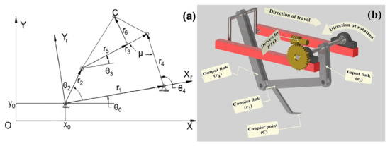
Figure 4.
Coupler point C on the coupler link of a four-bar mechanism: (a) a schematic view, reproduced from ref. [56] with permission from Copyright Frontiers Media S.A., and (b) a schematic 3D model.
In Section 4.5, the two objective functions defined here are formulated using the design variables and are further described.
4.4. The Constraints of Cultivator Design Problem
Given that the four-bar mechanism designed for the weeding operation is rear-mounted on the tractor and is driven by the PTO, its input link should be able to continuously rotate . To this end, the Grashof criterion is defined as:
In other words, the Grashof criterion states that the sum of the lengths of the longest and shortest links must be smaller than the sum of the lengths of the other two links. Note that this criterion guarantees the full rotation of two adjacent links. Besides meeting the Grashof criterion, the input link should also be the shortest link in order for a crank–rocker four-bar mechanism to have a full rotation at its input link. Grashof criterion is a common constraint and frequently presented in four-bar linkage studies [26,34,35,55], but the cultivator design problem has some other constraints that are unique and introduced in this study.
Regarding Figure 4a, constraint 2 avoids the collision between input link and the ground level.
Regarding Figure 4a, it can be concluded that constraint 3 keeps joint above the ground level.
Moreover, regarding Figure 4a, to avoid collision between output link and the ground level, Equation (11) must be satisfied.
where and i = 1 to 20. On the other hand, is not an independent design variable and is defined as a function of some other design variables in Section 4.5. In the above equation, represents the input angle at its first position corresponding to the first precision point and refers to the prescribed angle predefined by the designer for precision point. As can be seen, this study considers the synthesis process as a prescribed timing problem in which each precision point has a corresponding predefined angle that should be added to , so there exist 20 constraints that must be satisfied. The best prescribed angles () are obtained by a process of trial and error. Furthermore, to make sure that the precision points are tracked in the desired order, the following criterion should be fulfilled:
Imposing constraints 2 to 23 makes a clear distinction between common four-bar design problems and four-bar cultivator design problems, which leads to a smaller design space and more difficult search.
Another governing constraint of the design problem is the mechanism’s size limitation. The mechanism should have a reasonable size considering the manufacturing process, on the one hand, and its in-field application for weeding purposes on the other. This can be controlled by imposing bounds to the design variables (Table 2). Following Figure 4, in this table, to are related to the real links of the mechanism. The lower bounds for these links are defined 10 mm considering assembly limitations and the upper bounds are defined 450 mm in order to compare this study with other studies as this value is used as a reasonable size in the literature [14]. Furthermore, and refer to the intangible links of the mechanism used to define the exact position of coupler point in the synthesis process. Following Figure 4a, in Table 2, the negative values for are associated with the left-hand direction of vector and the negative values for are associated with the downward direction of vector . and are the base pin coordinates and, as can be seen, the lower bound of is selected to keep joint above the ground level. is the angle of the base link and, as mentioned before, is the input link angle in its first position corresponding to the first precision point. All sizes are in millimeters and angles are in degrees.
Table 2.
Limits of design variables.
With the design problem constraints being described, the multi-objective optimization problem can be expressed by (13).
Considering all constraints described above.
4.5. Four-Bar Mechanism Formulation
The schematic view of a four-bar mechanism is given in Figure 4a. The notations in the literature [33,35,36] are adopted for use in this study. Four-bar mechanism consists of three moving rigid links (, , ) plus one fixed link (). These links are connected by four pin joints, allowing relative rotation between adjacent links. The link is the link driven by the power source providing rotary motion (here, the PTO shaft of tractor) and called input link or crank. The link is called output link or rocker. The coupler link () connects the input link to the output link. Point c on the coupler link is called coupler point and its path during the input link rotation is known as coupler curve. In this study, the desired coupler curve is the one displayed in Figure 3. Therefore, proposed optimal design methods should determine independent design variables (e.g., mechanism dimensions, coordinates of the base pin and linkage angles) in order for coupler point to track this path. In practice, following the four-bar mechanism optimal design, the weeding blade should be mounted exactly at the coupler point. This section first explains (,) in Equation (6), which are coordinates of the coupler point, and then the dev(μ) function in Equation (7). According to Figure 4a:
The point’s location in the OXY coordinate system is as follows:
in Equations (14) and (15) is not an independent design variable and can be obtained from other design variables. Accordingly, the following vector loop equation can be expressed in the complex OXY coordinate system as:
The vector form of Equation (17) can be rewritten using complex designation:
By expanding Equation (18) and drawing on the equation of Freudenstein, can be eliminated and , a function of and some other design variables, can be easily solved and obtained. The linkage design literature has explained the extraction method of [57,58].
While:
The minus/plus sign in Equation (19) represents the two possible mechanical states of the mechanism. During the synthesis processes described in Section 4.6 and Section 4.7, both possible states should be synthesized and the better state should be selected. As a result, (,) and, thus, TE were obtained from 10 design variables.
The dev(µ) function can be defined as follows to give a clearer insight into the second objective function:
In Equation (22), is the maximum transmission angle, and shows its minimum during a full rotation of the input link. Both angles can be simply calculated based on the mechanism linkage lengths [49]:
As shown in Equation (22), the objective of the optimal design process is to reduce the deviation of the transmission angle from the right angle. If the highest deviation of the transmission angle from the right angle occurs at less than , the design process increases the angle; otherwise, it reduces the angle.
4.6. HGA-Based Optimal Design Process
4.6.1. Goal Attainment Method
Goal attainment is a classical method transforming a multi-objective problem into a scalar or single-objective problem. The method is a subtype of a broader method called weighted metric method [52,53,54,59,60].
Subject to constraints/Equations (3) to (5)
In the above equation, is the objective function. is the weight allocated to objective function by decision-maker where and and is a utopian value related to objective function and predefined by decision-maker. If p approaches ∞, the problem transforms into a ∞-norm problem and is called Chebyshev problem [53,54,59,60] or min-max method [54,55]. In that case, it is easy to prove that Equation (25) can be expressed as follows:
Subject to constraints/Equations (3) to (5)
Equation (26) can be easily rewritten in the form of Equation (27) in order for the numerical solvers to face this problem as a standard nonlinear constraint optimization problem.
Subject to constraints/Equations (3) to (5) and also subject to:
The step-by-step sequence of goal attainment method for implementation is as follows:
- (1)
- The decision-maker defines the vector of ideal objective functions (b). Each component of this vector represents a utopian value associated with a counterpart objective function. During the optimization process, the goal is that any objective function approaches its corresponding utopian value.
- (2)
- The decision-maker also defines the vector of weights (w). Each component of this vector represents a value associated with a counterpart objective function. The value of each component is in proportion to the importance of the corresponding objective function.
- (3)
- The optimization process tries to minimize the scalar α in order to minimize the gap between the ideal objective functions and real objective functions.
It can be easily shown that a set of non-inferior solutions can be obtained by varying the vector of weights. The geometrical illustration of goal attainment method for a problem with two objective functions can be found in Ref. [52]. Given vector w and b, the direction of search is determined. The intersection between vector b + α·w and the feasible region of search space defines the solution point. The goal attainment method in the form of Equations (27) and (28) was introduced into an engineering problem in 1975 [61]. The main advantage of this method is that it is appropriate for both convex and nonconvex optimization problems [61]. It is noteworthy that the decision-maker can scale the objective functions in the above-mentioned equations due to the fact that different objective functions have different order of magnitude. The scaling process is called the normalization of objectives. To this end, can be substituted for in Equations (25), (26) and (28).
In the above equation, is the normalized vector of objective functions, whereas and are minimum and maximum of , respectively. An easy-to-understand presentation on goal attainment method is given in the literature for the practically oriented readers [52,53,54]. On the other hand, more detailed explorations of this method are presented in the literature for the mathematically oriented readers [59,60].
4.6.2. Non-Dominated Sorting Genetic Algorithm (NSGA-II)
A non-dominated sorting genetic algorithm (NSGA-II) is one of the most popular and efficient multi-objective evolutionary algorithms. NSGA-II hybridized with goal attainment method was employed for multi-objective optimization in this study. In Section 2.1, it was discussed that the optimization process based on genetic algorithms is inspired from natural genetics. First, a number of possible solutions—called individuals or chromosomes—for the optimization problem are generated. A set of these individuals is called population. The algorithm then uses different operators (such as selection, crossover and mutation) over multiple generations to improve these solutions. Finally, the best optimal solution in the last generation is selected as the problem solution. Note that each individual in each generation is assessed by its fitness function (objective function). In GA, each individual (chromosome) is characterized by a set of genes. The number of the required genes depends on the design variables. On the other hand, the concept of NSGA-II is based on pareto front, a set of non-dominated solutions which are not superior to each other but are better than other solutions in the search space. In other words, there is no unique solution superior to other solutions considering all objective functions and each solution in pareto front makes a trade-off between the objective functions. NSGA-II as an efficient method has been used in the mechanism and machine design studies [36,62,63].
Considering (Ref. [62], see Figure 8) the step-by-step sequence of NSGA-II for implementation is as follows:
- (1)
- Randomly generate an initial population () of size N regarding the constraints governing the problem.
- (2)
- Evaluate the objective functions of each individual in .
- (3)
- Apply GA operators, such as selection, mutation and crossover, to produce the offspring population () of size N from .
- (4)
- Evaluate the objective functions of each individual in .
- (5)
- Combine and to produce of size 2N.
- (6)
- Classify the entire population of into different fronts based on non-dominated sorting method.
- (7)
- Form the new generation () of size N by individual from better fronts. Firstly, fill by the individuals of first front. Then, fill it by the individuals of second front, and so on. As there exist N slots in and, on the other hand, have 2N individuals, the extra fronts cannot transfer to new generation and must be eliminated. Regarding the last allowed front, calculate the crowding distance of each individual by Equation (30) [62] and transfer the individuals with highest values into the . The selection of individuals based on crowding distance keeps the diversity of new population.
- (8)
- Go to step 2 and repeat the procedure provided that the stopping criterion is not satisfied.
- (9)
- Stop and output the pareto solutions if the stopping criterion is satisfied.
The above equation, is the crowding distance of individual; k denotes the number of objective functions; and are the objective function of and individual, respectively; and represent the maximum and minimum of objective function, respectively.
The multi-objective evolutionary algorithms literature explains the full details of this method [54].
4.6.3. The Hybrid of NSGA-II and Goal Attainment Method
Figure 5 helps to understand the hybrid of NSGA-II and goal attainment method for this problem. This hybridization integrates the advantages of both methods [64]. First, regarding constraints 1 to 23, algorithm randomly generates the initial population , including 200 individuals. As earlier discussed in Section 4.5, this problem consists of 10 independent variables; therefore, each individual is composed of 10 genes and thus 10 corresponding values. The values corresponding to these genes are in fact the values corresponding to the problem design variables. The problem variables are:,,,,, , , , , . Following the evaluation of each individual to select appropriate ones by means of Equations (6) and (22), the algorithm begins to regenerate a new population of size 200 using genetic operators. In this study, tournament, adaptive feasible and heuristic function are used for selection, mutation and crossover, respectively. The selection function chooses parents to breed a new generation (using the crossover operator) based on their scaled fitness function values. Tournament function as a selection function chooses each parent by selecting a predefined number of individuals randomly, and then selecting the best individual among them to be a parent. The crossover operator is used to combine the characteristics of two parents to reproduce a new offspring for the next generation. Heuristic function returns a child that lies on the line containing the two parents, a small distance away from the parent with the better fitness value and in the direction away from the parent with the worse fitness value. The mutation operator makes small random changes in some individuals by altering one or more gene values, which leads to genetic diversity in order for the algorithm to search a larger space. In adaptive feasible function, directions are randomly generated with respect to the last successful or unsuccessful generation. Following the evaluation of each individual in the new population by means of Equations (6) and (22), the algorithm combines and to produce new population of size 400. At the next stage of the process, as can be seen in Figure 5, the new generation of size 200 is generated based on the fronts classification and crowding distance, which are discussed in Section 4.6.2, and then the algorithm evaluates whether the stopping criterion is satisfied or not. This iteration replicates in order for stopping criterion to satisfy. Next, the goal attainment method is run on the pareto front suggested by NSGA-II. Finally, the best solution is chosen among the trade-off solutions suggested by goal attainment method. Higher-level information is used to choose the best solution. The term higher-level information refers to the non-technical and experience-based information of the problem.
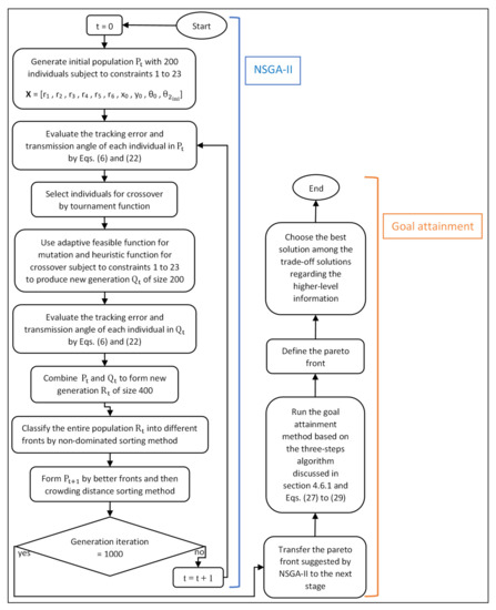
Figure 5.
Flowchart of HGA for the four-bar cultivator synthesis.
4.7. QNM-Based Optimal Design Process
In general, the numerical optimization methods first randomly pick a point (solution) across the design space and then follow an iterative process to drive this point toward the optimal point, with respect to the following relation, until the design criteria are met [65,66]:
In the above equation, k represents the iteration number, is the current design point and is the variations in the current design. As shown by Equation (31), detection of shifts in the current design point () toward a more optimal solution is itself made of two subproblems: the desirable search direction vector () over the design space, and the scalar value of the desirable step size () along this search direction.
The study used a quasi-Newton method, called BFGS, to determine the desirable search direction. In QNM methods, the first-order and second-order derivatives of the objective function are used to obtain the desirable search direction. An advantage of these methods over the ones that only use the first derivatives (gradients) of the objective function is their higher convergence rate. Another advantage is that information from the second derivatives (Hessians) of the objective function is estimated using the information from the first derivatives, and, unlike Newton methods, there is no need for computing the second derivatives. This substantially simplifies the implementation of QNMs and enhances their use in practice [65]. In this study, the gradient of the objective function was computed using the forward finite difference method. The correct step size was also determined from a polynomial interpolation method called Fletcher’s Linear Search (FLS) algorithm. The BFGS method and FLS algorithm can be observed in the optimization literature [65,66]. The overview is described in Appendix A.
The BFGS quasi-Newton algorithm is an unconstrained optimization method, whereas the cultivator design is a constrained optimization problem due to the upper and lower bounds of the design variables, the Grashof criterion and the constraints 2 to 23. The following parameter transformation can be used to ensure that all design variables are within their defined upper and lower bounds [43,44]:
In the above equation, is the design variable, is the search variable, and and are the upper and lower bounds of the design variable. From this equation, it can be found that the design variable remains between the upper and lower bounds when the search variable shifts between −∞ and +∞. This transformation, in fact, maps the set of limitless search variables onto the set of limited design variables, which is necessary for the design problem.
Equation (32) can be redefined as (33) [44]:
where and are the redefined upper and lower bounds of the design variable.
Due to the sequential transformation set [43] adapted for the cultivator design in this study, the above redefinition can be realized (Figure 6). By redefining the bounds of variables in this algorithm, it can be ensured that a crank–rocker Grashoft mechanism is synthesized with its input link being the shortest link and its base link being the longest one. As can be seen in Figure 6, depicts that 3 out of 10 design variables of the problem do not need the aforementioned redefinition due to the fact that the constraints governing the problem are not dependent on these three variables. As a consequence, the algorithm calculates them by Equation (32). Then, the algorithm calculates as the shortest link of the mechanism. At the next stage of the process, to ensure a Grashof crank–rocker mechanism, the upper and lower bounds of , and are redefined, and, after redefinition process, these three variables will be calculated by Equation (33). As the flowchart clearly illustrates, these redefinitions ensure that the sum of the lengths of the longest and shortest links ( and ) is smaller than the sum of the lengths of the other two links ( and ). As discussed in Section 4.4, this criterion is necessary to have a continuous rotary input, and, on the basis of the fact that the above algorithm defines the input link as the shortest link, this link has a continuous rotation and can be driven by the PTO shaft of tractor. Finally, the upper and lower bounds of the remaining three design variables (, , ) are redefined based on constraints 2 to 23 described in Section 4.4, and these variables are calculated by Equation (33). In simpler terms, the algorithm of the sequential transformation set converts the constrained optimization problem to an unconstrained one. Therefore, the unconstrained quasi-Newton BFGS method can be employed to solve this problem.
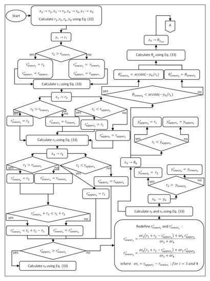
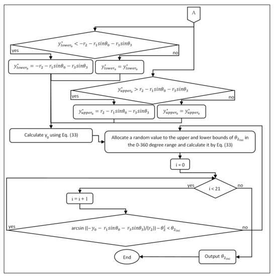
Figure 6.
Flowchart of sequential transformation set for the four-bar cultivator synthesis.
In this section, a multi-objective optimal design method was implemented using weighted sum approach in which a specific weight was allocated to each fitness function (objective function). This approach is popular, makes the problem more flexible and easier to solve and has been employed frequently in the literature [67,68,69,70]. In simpler terms, the multi-objective optimization problem being described by Equation (13) can be rewritten as follows:
Considering Table 2 and all constraints described in Section 4.4.
Where w1 and w2 are allocated weights to TE and TA, respectively. Due to the same importance of both fitness functions, the weight value of 1 was used for both of them. Results are given and discussed in Section 6.
5. Experimental Study
To evaluate and quantify the effectiveness of the proposed methods, an optimal mechanism was developed, and a field experiment was carried out on a sandy loam soil in an eggplant field located near Zarqan—a city close to Shiraz, Iran. The nominal plot size was 12 × 4 m. The proposed mechanisms, which were designed for in-field operation, should be mounted on a tractor and driven by a PTO. However, the prototype developed for this study was pulled by an operator and powered by a gearmotor. The rotational speed of the gearmotor was set by an inverter and checked by a tachometer, whereas a stopwatch was used to measure the operation time for a 12-m-long furrow in order for the forward speed of the mechanism to be calculated and set. Three performance indicators, briefly discussed below, were evaluated and compared with other studies.
5.1. Cultivation Depth
As mentioned in Section 1, there is an ideal range for the cultivation depth of weeding cultivators. As discussed in previous sections, the cultivator will cause damage to crop roots or have low weeding performance if its weeding blade works out of this range. Hence, cultivation depth is an important performance indicator and should be measured in order for the design method to be practically assessed. A steel ruler was used to measure the cultivation depth of the developed mechanism.
5.2. Weeding Performance
Weeding performance is a key indicator of cultivators, which reflects the capability of mechanism to control weeds and is calculated by Equation (35) [25,47].
where and are the number of weeds after and before weeding operation, respectively. The higher the weeding performance is, the better the cultivator is.
5.3. Mechanical Damage
It is obvious that low mechanical damage to crop roots is another important indicator in order for a weeding cultivator to be recognized as a suitable implement for weed management. Mechanical damage is calculated by Equation (36) [47].
where is the number of safe crop plants after weeding operation and is the number of crop plants before weeding operation. The lower the mechanical damage is, the better the cultivator is.
6. Results and Discussion
The following steps were followed in order to obtain the proposed mechanisms in Section 4.6 and Section 4.7, and in order to verify the plausibility of these mechanisms for weeding operation: (1) the HGA-based and QNM-based methods were implemented in (the MathWorks Inc., Natick, MA, USA) to synthesize two different mechanisms. (2) To validate these mechanisms, some design indicators of them, such as tracking error function, transmission angle’s deviation from right angle (90 degrees) and the effective stroke of their blades, were compared with each other and with other existing studies employing different methodologies to design a four-bar mechanism for weed management. The importance of these design indicators was described in Section 2.2 and Section 3. (3) In order to observe the paths synthesized while the mechanisms are traveling and in order to further the verification of the proposed mechanisms, Working Model 2D was employed to simulate the synthesized mechanisms dynamically. The paths tracked in its graphical user interface were considered as a benchmark for comparison with the paths tracked by the designed mechanisms in MATLAB. (4) At the final stage, a mechanism was developed for on-site experiments, and its performance indicators, namely cultivation depth, weeding performance and mechanical damage to roots, were compared with four-bar cultivators presented in other studies and with conventional tools previously recorded in the literature.
A computer program was developed in MATLAB for the objective functions introduced in Section 4.3 and Section 4.5, and another one for the constraints introduced in Section 4.4 was developed in order to implement the HGA-based optimization problem. Both these programs were then transferred and performed in the Optimization Toolbox of MATLAB. Fifty runs were done with the different values of GA parameters. The results were simultaneously stored and compared. The parameters corresponding to the best run are shown in Table 3. Figure 7 shows a set of non-dominated optimal solutions or a pareto front, which represents trade-off solutions between two conflicting objective functions (AE and TA) so that a designer can select a solution suitable for the problem’s requirements. In this figure, point A and point B stand for the best AE and TA, respectively. AE refers to average tracking error and is obtained from the following equation:
Table 3.
Parameters of GA.
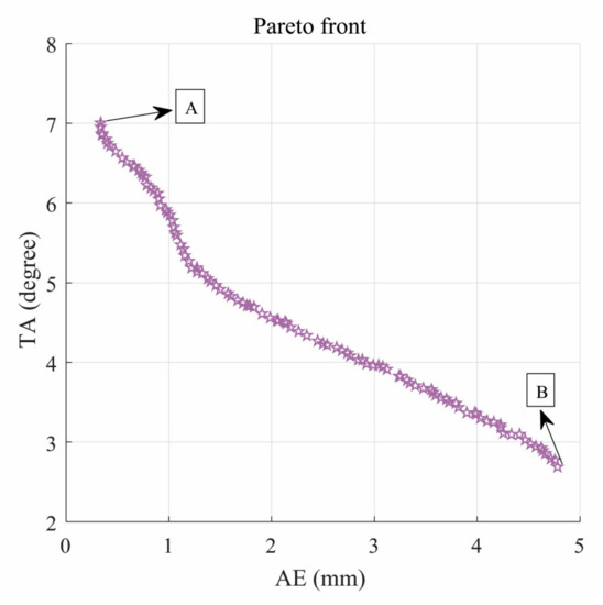
Figure 7.
The best fitness function over the entire run of GA-based optimization process.
In (37), TE is the tracking error from Equation (6), and N represents the number of precision points (=20). Although point A and point B have no superiority over each other from a mathematical perspective, point A was selected as the suitable one for the cultivator design problem in this study since it is a comparable solution to the solution proposed by the QNM-based method. It should be noted that, although point B has an ideal TA, its AE is practically unreasonable in comparison with the QNM-based method. On the other hand, the FLS algorithm, BFGS method and sequential transformation set were developed and implemented in MATLAB in order to solve the QNM-based method based on the requirements of the cultivator design problem. Figure 8 depicts how search variables and design variables change over the QNM-based optimization process. In addition, a deeper review of Figure 8b reveals how parameter transformations, presented in Section 4.7, keep the values of design variables between their upper (450) and lower (−450) bounds. For the purpose of illustration, the values of over the QNM-based optimization process are shown in Figure 9 (the straight lines at the top and bottom of the figure present the upper and lower bounds for —having been previously defined in Table 2). The plots corresponding to the other design variables are not presented here for the sake of brevity.
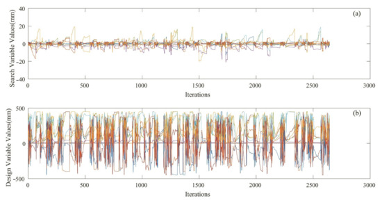
Figure 8.
(a) Search variables over the entire run of QNM-based optimization process, and (b) design variables over the entire run of QNM-based optimization process.
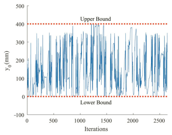
Figure 9.
The values of design variable over the entire run of QNM-based optimization process.
6.1. Generated Mechanisms and Paths
Figure 10 shows the synthesized mechanisms by both the HGA and QNM methods. The design variables of these two mechanisms and the mechanism synthesized using pareto multi-objective GA, without hybridization, are given in Table 4. Figure 11 shows the synthesized paths by HGA and QNM. A deeper review of Figure 11 reveals that the coupler point of both mechanisms successfully tracked the desired path of the weeding operation. As discussed in Section 1, the weeding depth of cultivators should be over 30 mm and should not exceed 40 mm [19,25]. It means that the weeding blades of both mechanisms work within the ideal range through the soil, which reduces the risk of physical damage to roots. Table 5 lists the information on the proposed mechanisms and the mechanisms described in two other papers [14,25] for further comparison.
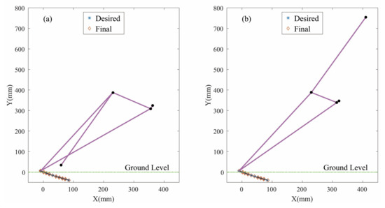
Figure 10.
(a) HGA-based synthesized mechanism, and (b) QNM-based synthesized mechanism.
Table 4.
Final results of the synthesized mechanisms.
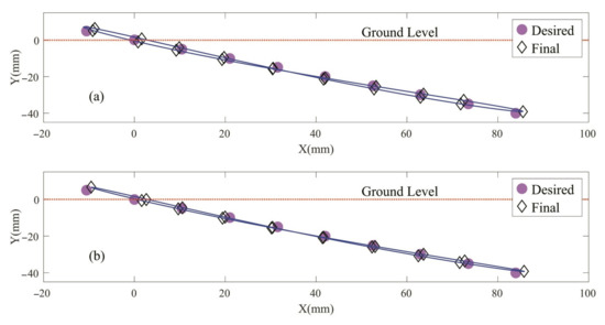
Figure 11.
(a) HGA-based synthesized path, and (b) QNM-based synthesized path.
Table 5.
Comparative results between proposed and classic methods in terms of design indicators.
6.2. Average Tracking Error
From Table 5, it can be found that the AEs of the proposed mechanisms have no difference with each other, which means they perform equally in this respect. Given that the mechanism proposed in Ref. [14] was synthesized using the analytical–graphical method with three precision points, and the design method of the mechanism developed by the Rural Development Administration of Republic of Korea (RDA) [25] is not given, AE cannot be calculated for these mechanisms. However, AE is an indicator of tracking error, and, considering that the paths tracked by those mechanisms are far from the desired path, it can be concluded that the tracked paths had a considerable deviation from the desired path. To illustrate the point, consider that the effective stroke of the path tracked by the mechanism designed in Ref. [14] is 125 mm and the penetration depth is 30 mm, whereas the desired path shown in Figure 1 has a 102.5 mm longitudinal stroke and 40 mm penetration depth. Moreover, most of the time of this mechanism’s blade is out of the soil during one cycle. The blade of the mechanism evaluated and simulated in Ref. [25] only had a spot impact on the soil surface, which means that neither the longitudinal stroke nor the penetration depth is suitable for weeding operation.
6.3. Transmission Angle’s Deviation from Right Angle (TA)
From Table 5, it can be found that the largest deviation of the transmission angle from the right angle is , and in the GA-based, HGA-based and QNM-based synthesized mechanisms, respectively. These deviations occur at for GA-based, for HGA-based and for the QNM-based mechanism. These results show that HGA outperformed GA and QNM in the optimization of the transmission angle. However, since the transmission angle deviation in these methods remained far below the allowable limit (), the proposed mechanisms had satisfactory energy and torque transmission and would work smoothly. On the contrary, the highest deviations of the transmission angle from right angle for the mechanisms studied in Refs. [14,25] were and , occurring at and angles, respectively. Although the transmission angle of the mechanism designed in Ref. [14] remains in the allowable range () within one full rotation of the input link, it nears the boundary value. On the other hand, the mechanism studied in Ref. [25] exceeds the allowable range. In brief, the proposed methods in this study were successful in multi-objective optimization and optimized both objective functions (i.e., TE and TA) in line with the design goals.
6.4. The Effective Stroke of Weeding Blade
From Table 5, it can also be concluded that the effective strokes of the mechanisms developed and studied in Refs. [14,25] are only and , whereas the proposed mechanisms of this study have of effective stroke. The effective stroke in Table 5 is an indicator of the blade’s travel time through the soil during a weeding cycle. The low value of this indicator means that the blade has spent a considerable proportion of its travel time out of the soil within one full rotation of the input link, which is the wasted part of a weeding cycle [25]. The ideal values of this indicator for the proposed mechanisms are because of the fact that the mechanisms in this study had no limitations in the number of precision points, and a suitable number of precision points were selected—most of which were below the surface—to ensure a considerably large effective stroke for the weeding blade. On the contrary, the analytical–graphical methods impose a limitation on the number of precision points, which, in turn, forces the designers to select their best tracked path from a number of paths provided by their design method. These best paths had and of ineffective stroke in Refs. [14,25], respectively.
6.5. The Results of Dynamic Simulation
For dynamic analysis, the HGA-based and QNM-based proposed mechanisms were simulated in Working Model 2D. As outlined earlier, due to the well-tried record and high acceptance of this simulation software, the paths tracked in its graphical user interface were considered as a benchmark for the further verification of the proposed methods. On the basis of this simulation, we can study the motion behavior of both proposed cultivators, and it can lead to the further verification of these mechanisms. The results are given in Figure 12 and Figure 13. Figure 12b and Figure 13b show the tracked paths of both mechanisms in their static states in the software. As can be seen, these paths are similar to those in Figure 11a,b, respectively. Then, the tracked paths in the dynamic states of the mechanisms at different travel speeds (2, 4, 6 and 8 km ) are shown (Figure 12c–f and Figure 13c–f). From these figures, it can be found that the travel speed can be raised to 6 km , although both mechanisms were designed based on a travel speed of 2 km . Figure 12f and Figure 13f suggest that the mechanisms had no satisfactory overlap in their penetration strokes at 8 km . As a result, they are not suitable for weeding operation at this travel speed. Due to the above discussion, it is clear that, at 2 km , the penetration stroke of the blade is closer to its return stroke. That is, the average linear speeds during the penetration and return strokes are closer, providing a more uniform linear speed at the tip of the weeding blade, which is an advantage. As can be seen, another advantage of this travel speed for the proposed mechanisms is associated with more satisfactory overlap in their penetration strokes, which can improve weeding efficiency. This result corroborates the results of other studies done on this topic, which state that a decrease in the travel speed of the cultivator at a constant rotational speed of the input link can enhance the weeding efficiency [25,47]. It should be considered that, in Figure 12c–f and Figure 13c–f, the travel speed of the cultivators increased while the rotational speed of the input links was kept constant. In practice, in order for these conditions to happen, the PTO shaft of the tractor should be set in independent mode, in which the RPM of the PTO is irrespective of the travel speed of the tractor. As discussed in Section 4.1, in general, the travel speed is recommended to be constant for weeding operation. However, if the operator wants to increase the travel speed during weeding operation, the tractor PTO must be set in the transmission driven mode. In this case, the tractor throttle will be set to a fixed value, and the travel speed must be changed by shifting gears during the operation. Any change in the travel speed will translate into a change in the rotational speed of the PTO, and the ratio of the tractor travel speed to the rotational speed of the input link—which is extensively discussed in Section 4.1—so the ratio of the tractor travel speed to mean linear speed of the coupler point (weeding blade) will remain constant. This is because the input link is driven by the PTO shaft of the tractor. To put it another way, in this case, the PTO shaft (and, hence, the input link) is coupled to the wheel speed of the tractor to ensure a constant relationship between the travel speed and the rotational speed of the input link.
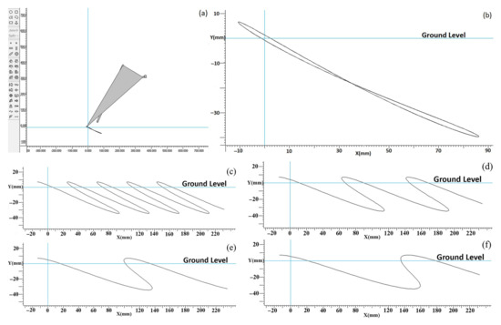
Figure 12.
HGA-based synthesized mechanism in Working Model 2D software: (a) simulated mechanism, (b) the side view of the tracked path in the static state of the mechanism, (c–f) the side view of the tracked paths in the dynamic states of the mechanism at different travel speeds, respectively, are 2 km , 4 km , 6 km , 8 km .
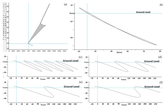
Figure 13.
QNM-based synthesized mechanism in Working Model 2D software: (a) simulated mechanism, (b) the side view of the tracked path in the static state of the mechanism, (c–f) the side view of the tracked paths in the dynamic states of the mechanism at different travel speeds, respectively, are 2 km , 4 km , 6 km , 8 km .
6.6. Experimental Results
As discussed in Section 5, three major performance indicators, namely cultivation depth, weeding performance and mechanical damage to crop roots, were evaluated in situ to assess the in-field capability of the developed mechanism. Figure 14 shows the developed prototype in situ.
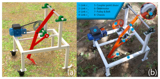
Figure 14.
The four-bar cultivator: (a) 3D model, and (b) developed prototype.
As mentioned in Section 1, the ideal range for the cultivation depth of weeding cultivators is from 30 mm to 40 mm [19,25]. If the weeding blade exceeds 40 mm, it will increase the risk of damage to crop roots. On the other hand, it will pose a challenge to weed control if the weeding blade works lower than 30 mm. The displacement and velocity vector analysis presented in Section 4.1 identified the weeding blade’s path and guaranteed the optimal cultivation depth theoretically. To evaluate the cultivation depth in situ, fifteen points were checked and measured by a steel ruler at random, and the observed values were from 35 mm to 40 mm. These in situ values were within the ideal range. However, as can be seen in Figure 3 and Figure 11, the optimal depth theoretically defined and obtained in this study was 40 mm, whereas the mechanism worked between 35 mm and 40 mm in practice. This little difference in value between theory and practice can be attributed to the ground unevenness. The problem of ground unevenness can be resolved if the mechanism will be mounted on a tractor. As discussed in Section 4.1, the mechanism was designed to be mounted on a tractor, while the developed prototype was pulled by an operator in this study. Nonetheless, the difference in value between theory and practice was reasonable because the mechanism worked within the ideal range.
Four treatments were undertaken to evaluate the weeding performance and mechanical damage to crop plants. Three replications were completed for each treatment and three sample areas were chosen at random for each replication. Each sample area for weeding performance was a 2-m-long furrow (=around 200 mm * 2000 mm) and for mechanical damage was a 2-m-long ridge. Both indicators were calculated by averaging the obtained values. The treatments were as follows:
Treatment (state) 1: forward speed = 1 km
Treatment (state) 2: forward speed = 2 km
Treatment (state) 3: forward speed = 4 km
Treatment (state) 4: forward speed = 4 km ; the ratio between the tractor travel speed to the rotational speed of the input link and, hence, to the mean linear speed of the weeding blade in state 4 was set the same as this ratio in state 2.
Treatment 2 is the one based on which the mechanism was designed. In Section 4.1, it was extensively discussed that, to increase the forward speed of a tractor, it is necessary to set the tractor PTO in transmission driven mode rather than independent mode. As we know, in former mode, the RPM of the PTO increases in proportion to the forward speed of the tractor, whereas, in latter mode, the RPM is irrespective of the forward speed. Hence, in transmission driven mode, the speed ratio between tractor travel speed and rotational speed of PTO will be maintained constant and, theoretically, the weeding blade of the mechanism will track the path shown in Figure 3. In this case, the field capacity increases due to the increase in forward speed. Treatment 4 was a representative sample of such cases. Nevertheless, due to ground unevenness in the real fields, it is possible to have slight variation in the above-mentioned ratio, although the PTO was set in transmission driven mode. Treatment 1 and 3 study the behavior of the designed cultivator in such conditions in the real-life operations.
As can be seen in Table 6, the proposed four-bar cultivator in state 2—based on which the mechanism was designed—reached 94% weeding performance, calculated by Equation (35), and caused 3% mechanical damage to crop plants, calculated by Equation (36). The modes of action of the cultivator were cutting for most of the well-established weeds and uprooting and burial for most of the young weeds. The mechanism damaged the crop plants that were not planted on top of the ridges and planted very close to the furrows, so it is important to have high accuracy in the planting stage. The mechanism also cannot properly cope with the weeds grown in the margins of furrows. This problem can be addressed if a wider blade is applied, although it increases the risk of mechanical damage to crop roots. However, from Table 6, it can be concluded that, in terms of weeding performance, the proposed four-bar cultivator in state 2 is better than most of the conventional tools and four-bar cultivators designed or evaluated in other studies. It can also be concluded that the proposed mechanism is less effective than ducksfoot and a rotary powered cultivator. However, both of them would pose problems on young crop plants if operated in narrow rows because of their vigorous soil movement [17]. As extensively discussed in Section 2.2 and Section 4.1, the proposed mechanism was designed to imitate the hand motion of farmers and track a predefined path in order for crop plants to be kept safe, whereas the conventional tools plough the soil indiscriminately. In this study, the narrow rows with the width of about 300 mm were prepared to test the capability of the proposed mechanism in narrow furrows, and, as can be seen in Table 6, the developed prototype was successful to work in narrow rows. Figure 15 shows a sample area before and after weeding operation. The superiority of the developed four-bar cultivator over four-bar cultivators in other studies [25,47] can be attributed to two main reasons. Firstly, thanks to optimization techniques, the design method applied enough precision points to track the desired path, whereas the classic methods had been faced with the problem of limited precision points. Secondly, as described in Section 4.1, this study introduced the cultivator’s forward speed to design a process to neutralize its adverse effect on the path generation problem, whereas other studies synthesized the mechanism in its stationary state, which produced a serious path-generating error.
Table 6.
Comparative results between proposed mechanism and other studies in terms of performance indicators.
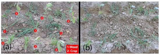
Figure 15.
A sample area: (a) before weeding, and (b) after weeding.
From state 1 to state 3, it can also be concluded that a decrease in forward speed at a constant rotational speed enhanced weeding performance, and this agrees with other studies [25,47]. As can be seen in Figure 12 and Figure 13, this enhancement can be attributed to better overlaps between penetration strokes at lower forward speeds. On the other hand, this decrease led to higher mechanical damage to crop plants, and this confirms other findings [47], so there is a trade-off between weeding performance and mechanical damage at the speed of 2 km per hour. As mentioned in Section 4.1, it is important to note that the mechanism was designed based on the forward speed of 2 km per hour to track the desired path. On the other hand, the field capacity is dependent on forward speed. The higher the forward speed is, the higher the field capacity is. To increase the forward speed without any effect on the weeding blade’s path, the tractor PTO should be set in the transmission driven mode. In this case, the ratio of the tractor forward speed to mean linear speed of the weeding blade relative to the tractor reference, which defines the blade’s path, will remain constant. By vector analysis, it was extensively discussed in Section 4.1 why this occurs. To evaluate this in situ, treatment 4 was undertaken. The mechanism was simulated in Working Model before on-site experiments to reach the desired rotational speed of the gearmotor, and it was set using an inverter in situ. As can be seen in Table 6, the weeding performance and mechanical damage in states 2 and 4 were different, and it is not clear why this occurred because the mechanism’s blade in both of these states should track the same path, theoretically. It may be associated with the aggressiveness of these two states. Although the mechanism’s blade tracks the same path in both states, the mechanism is more aggressive in state 4 and can cause higher weeding performance and mechanical damage. Nevertheless, as far as in-field application is concerned, the difference in value between these two states is reasonable.
7. Conclusions and Further Studies
A four-bar mechanism was developed using a quasi-Newton method (QNM) and hybrid genetic algorithm (HGA) as multi-objective optimization methods to meet the weeding requirements. The advantages of the proposed mechanism are as follows:
- (1)
- The proposed methods synthesized an active tool powered by PTO, which avoids waste of energy through the drawbar of the tractor.
- (2)
- A predefined path, inspired by the hand motion of farmers during hand weeding, was introduced to the mechanism synthesis process so that the weeding blade tracked a targeted path and did not exceed the allowable depth (40 mm), which reduces the risk of mechanical damage to the crop roots.
- (3)
- The maximum closeness of penetration and return stroke of the blade, achieved through displacement and velocity vector analysis, tries to maximize weeding efficiency. On the contrary, conventional cultivators indiscriminately plough the soil, which can lead to a large amount of soil disturbance.
- (4)
- Unlike the analytical–graphical approaches formerly used to synthesize four-bar mechanisms for weeding, the proposed methods in this study overcame the limited-precision-point problem, which leads to synthesizing a four-bar mechanism whose blade is capable of tracking a more precise path through the soil.
- (5)
- Compared with the transmission angle’s deviation of the mechanisms developed based on analytical–graphical approaches in Refs. [14,25], that of the proposed mechanism has decreased by 85.2% and 88.9%, respectively. The decrease in the value of the transmission angle’s deviation from a right angle (90 degrees) is an indicator of smooth rotations in the joints of a four-bar mechanism and then good torque and energy transmission.
- (6)
- Compared with the effective stroke of the mechanisms developed based on analytical–graphical approaches in Refs. [14,25], that of the proposed mechanism has increased by 113% and 300%, respectively. The effective stroke of the weeding blade is an indicator of the interaction time between the weeding blade and soil during a weeding cycle.
- (7)
- In terms of weeding performance and mechanical damage to crop plants, the proposed mechanism is more effective than conventional tools and four-bar cultivators developed based on classic methods.
Furthermore, due to the fact that this study aimed to improve the design and performance indicators of a cultivator, namely tracking error, transmission angle, weeding performance, mechanical damage and cultivation depth, further studies are needed to investigate the energy consumption of four-bar cultivators, which is out of the scope of this research. As mentioned before, evidence in the literature supports the hypothesis that, in comparison with conventional passive tools, active tools are more efficient in terms of energy consumption. Consequently, it is necessary to investigate the energy consumption of the four-bar cultivator as an active tool in further studies. Moreover, the force analysis of the mechanism’ blade, which works through the soil, is useful and can be applied to another study.
Author Contributions
Conceptualization, H.H. and A.F.; methodology, H.H.; software, H.H., F.M. and A.N.; validation, H.H., A.F. and A.N.; formal analysis, H.H.; investigation, H.H. and A.N.; resources, H.H., A.F. and A.N.; data curation, H.H. and F.M.; writing—original draft preparation, H.H.; writing—review and editing, A.F., A.N. and O.H.; visualization, H.H.; supervision, A.F., O.H. and A.N.; project administration, H.H. and A.N. All authors have read and agreed to the published version of the manuscript.
Funding
This research received no external funding.
Institutional Review Board Statement
Not applicable.
Informed Consent Statement
Not applicable.
Data Availability Statement
Not applicable.
Conflicts of Interest
The authors declare no conflict of interest.
Appendix A. BFGS Algorithm with FLS
The overview of the Broyden–Fletcher–Goldfarb–Shanno (BFGS) algorithm employed in Section 4.7 is described here:
Step 1: Estimate an initial design point . Set the initial Hessian of the objective function and set k = 0. Input convergence criteria and compute the gradient vector as:
Step 2: If convergence criteria are satisfied, stop the iterative process. Output and .
Step 3: Solve the following linear system of equations to obtain the search direction :
Step 4: Use FLS (Fletcher’s line search) algorithm to obtain αk that minimizes
Step 5: set:
Step 6: Update the Hessian approximation:
where the correction matrices and are given as:
Step 7: Set k = k + 1 and go to step 2.
In the above algorithm, is a n by n identity matrix and n is the number of search variables. is change in gradient and is change in search point, and k is the number of iterations.
References
- Bohne, B.; Hensel, O. Application of thermoplastics to increase efficiency during thermal weed control. Landtechnik 2012, 67, 441–444. [Google Scholar] [CrossRef]
- Mohidem, N.A.; Che’Ya, N.N.; Juraimi, A.S.; Ilahi, W.F.F.; Roslim, M.H.M.; Sulaiman, N.; Saberioon, M.; Noor, N.M. How can unmanned aerial vehicles be used for detecting weeds in agricultural fields? Agriculture 2021, 11, 1004. [Google Scholar] [CrossRef]
- Chang, C.; Xie, B.; Chung, S. Mechanical control with a deep learning method for precise weeding on a farm. Agriculture 2021, 11, 1049. [Google Scholar] [CrossRef]
- Gharde, Y.; Singh, P.K.; Dubey, R.P.; Gupta, P.K. Assessment of yield and economic losses in agriculture due to weeds in India. Crop Prot. 2018, 107, 12–18. [Google Scholar] [CrossRef]
- Pannacci, E.; Tei, F.; Guiducci, M. Evaluation of mechanical weed control in legume crops. Crop Prot. 2018, 104, 52–59. [Google Scholar] [CrossRef]
- Tellaeche, A.; Pajares, G.; Burgos-Artizzu, X.P.; Ribeiro, A. A computer vision approach for weeds identification through support vector machines. Appl. Soft Comput. 2011, 11, 908–915. [Google Scholar] [CrossRef]
- Rob, M.M.; Hossen, K.; Khatun, M.R.; Iwasaki, K.; Iwasaki, A.; Suenaga, K.; Kato-Noguchi, H. Identification and Application of Bioactive Compounds from Garcinia xanthochymus Hook. for Weed Management. Appl. Sci. 2021, 11, 2264. [Google Scholar] [CrossRef]
- Zhang, X.; Chen, Y. Soil disturbance and cutting forces of four different sweeps for mechanical weeding. Soil Tillage Res. 2017, 168, 167–175. [Google Scholar] [CrossRef]
- Le Bellec, F.; Velu, A.; Fournier, P.; Le Squin, S.; Michels, T.; Tendero, A.; Bockstaller, C. Helping farmers to reduce herbicide environmental impacts. Ecol. Indic. 2015, 54, 207–216. [Google Scholar] [CrossRef]
- Carrubba, A.; Militello, M. Nonchemical weeding of medicinal and aromatic plants. Agron. Sustain. Dev. 2013, 33, 551–561. [Google Scholar] [CrossRef]
- Melander, B.; Lattanzi, B.; Pannacci, E. Intelligent versus non-intelligent mechanical intra-row weed control in transplanted onion and cabbage. Crop Prot. 2015, 72, 1–8. [Google Scholar] [CrossRef]
- Nieuwenhuizen, A.T.; Tang, L.; Hofstee, J.W.; Muller, J.; van Henten, E.J. Colour based detection of volunteer potatoes as weeds in sugar beet fields using machine vision. Precis. Agric. 2007, 8, 267–278. [Google Scholar] [CrossRef][Green Version]
- Nieuwenhuizen, A.T.; Hofstee, J.W.; van Henten, E.J. Performance evaluation of an automated detection and control system for volunteer potatoes in sugar beet fields. Biosyst. Eng. 2010, 107, 46–53. [Google Scholar] [CrossRef]
- Hosseini, A.A.M.; Akhijahani, H.S.; Mehravar, H.; Massah, J. Design of a mechanism for a new cultivator (part 1: Path generation and dimensional synthesis). Agric. J. 2007, 9, 63–76, (In Persian, with English abstract). [Google Scholar]
- Nosrattia, I.; Sabeti, P.; Chaghamirzaee, G.; Heidari, H. Weed problems, challenges, and opportunities in Iran. Crop Prot. 2020, 134, 104371. [Google Scholar] [CrossRef]
- O’Dogherty, M.J.; Godwin, R.J.; Dedousis, A.P.; Brighton, J.L.; Tillett, N.D. A mathematical model of the kinematics of a rotating disc for inter- and intra-row hoeing. Biosyst. Eng. 2007, 96, 169–179. [Google Scholar] [CrossRef]
- Pullen, D.W.M.; Cowell, P.A. An Evaluation of the Performance of Mechanical Weeding Mechanisms for use in High Speed Inter-Row Weeding of Arable Crops. J. Agric. Eng. Res. 1997, 67, 27–34. [Google Scholar] [CrossRef]
- Sedara, A.M.; Sedara, O.S. A review on inter-row crops mechanical weeder. Turk. J. Agric. Eng. Res. 2020, 1, 200–221. [Google Scholar]
- Cloutier, D.C.; van der Weide, R.Y.; Peruzzi, A.; Leblanc, M.L. Mechanical Weed Management. In Non-Chemical Weed Management: Principles, Concepts and Technology; Upadhyaya, M.K., Blachshaw, R.E., Eds.; CAB International: Oxfordshire, UK, 2007; pp. 111–134. [Google Scholar]
- Van der Linden, S.; Mouazen, A.M.; Anthonis, J.; Ramon, H.; Saeys, W. Infrared laser sensor for depth measurement to improve depth control in intra-row mechanical weeding. Biosyst. Eng. 2008, 100, 309–320. [Google Scholar] [CrossRef]
- Bowman, G. Steel in the Field: A Farmer’s Guide to Weed Management Tools; Sustainable Agriculture Network: Beltsville, MD, USA, 2002. [Google Scholar]
- Mohler, C.L. Mechanical management of weeds. In Ecological Management of Agricultural Weeds, Liebman, M., Mohler, C.L., Staver, C.P., Eds.; Cambridge University Press: Cambridge, UK, 2004; pp. 139–209. [Google Scholar]
- Prasertkan, K.; Usaborisut, P. Power requirements of combination tillage tool operating on two different fields. In Proceedings of the 110th The IRES International Conference, Osaka, Japan, 27–28 April 2018; pp. 25–29. [Google Scholar]
- Rao, N.R.N.V.G.; Chaudhary, H.; Sharma, A.K. Design and development of vibratory cultivator using optimization algorithms. SN Appl. Sci. 2019, 1, 1287. [Google Scholar] [CrossRef]
- Kwon, T.H.; Ashtiani-Araghi, A.; Lee, C.; Kang, T.G.; Lee, B.; Rhee, J. Evaluation of a crank-type walking cultivator for upland farming. J. Biosyst. Eng. 2014, 39, 1–10. [Google Scholar] [CrossRef]
- Khorshidi, M.; Soheilypour, M.; Peyro, M.; Atai, A.; Shariat Panahi, M. Optimal design of four-bar mechanisms using a hybrid multi-objective GA with adaptive local search. Mech. Mach. Theory 2011, 46, 1453–1465. [Google Scholar] [CrossRef]
- Kim, J.W.; Seo, T.; Kim, J. A new design methodology for four-bar linkage mechanisms based on derivations of coupler curve. Mech. Mach. Theory 2016, 100, 138–154. [Google Scholar] [CrossRef]
- Thomas, E.V. Development of a mechanism for transplanting rice seedlings. Mech. Mach. Theory 2002, 37, 395–410. [Google Scholar] [CrossRef]
- Jiang, Y.; Bian, B.; Li, L. Integrated harvest and farm-to-door distribution scheduling with postharvest quality deterioration for vegetable online retailing. Agronomy 2019, 9, 724. [Google Scholar] [CrossRef]
- Jamal, A.; Linker, R. Genetic operator-based particle filter combined with markov chain monte carlo for data assimilation in a crop growth model. Agriculture 2020, 10, 606. [Google Scholar] [CrossRef]
- Hwang, S.; Park, J.; Lee, J.; Shim, S.; Nam, J. Optimization of main link lengths of transplanting device of semi-automatic vegetable transplanter. Agriculture 2020, 10, 1938. [Google Scholar] [CrossRef]
- Zhao, X.; Guo, J.; Li, K.; Dai, L.; Chen, J. Optimal design and experiment of 2-DoF five-bar mechanism for flower seedling transplanting. Comput. Electron. Agric. 2020, 178, 105746. [Google Scholar] [CrossRef]
- Cabrera, J.A.; Simon, A.; Prado, M. Optimal synthesis of mechanisms with genetic algorithms. Mech. Mach. Theory 2002, 37, 1165–1177. [Google Scholar] [CrossRef]
- Calva-Yanez, M.B.; Nino-Suarez, P.A.; Portilla-Flores, E.A.; Aponte-Rodriguez, J.A.; Santiago-Valentin, E. Reconfigurable mechanical system design for tracking an ankle trajectory using an evolutionary optimization algorithm. IEEE Access 2017, 5, 5480–5493. [Google Scholar] [CrossRef]
- Lin, W.Y. A GA–DE hybrid evolutionary algorithm for path synthesis of four-bar linkage. Mech. Mach. Theory 2010, 45, 1096–1107. [Google Scholar] [CrossRef]
- Nariman-Zadeh, N.; Felezi, M.; Jamali, A.; Ganji, M. Pareto optimal synthesis of four-bar mechanisms for path generation. Mech. Mach. Theory 2009, 44, 180–191. [Google Scholar] [CrossRef]
- Chanekar, P.V.; Ghosal, A. Optimal synthesis of adjustable planar four-bar crank-rocker type mechanisms for approximate multi-path generation. Mech. Mach. Theory 2013, 69, 263–277. [Google Scholar] [CrossRef]
- Krishnamurty, S.; Turcic, D.A. Optimal synthesis of mechanisms using nonlinear goal programming techniques. Mech. Mach. Theory 1992, 27, 599–612. [Google Scholar] [CrossRef]
- Felezi, M.E.; Vahabi, S.; Nariman-zadeh, N. Pareto optimal design of reconfigurable rice seedling transplanting mechanisms using multi-objective genetic algorithm. Neural Comput. Appl. 2016, 27, 1907–1916. [Google Scholar] [CrossRef]
- Molari, G.; Mattetti, M.; Guarnieri, A. Optimal three-point hitch design to maximize lifting performance. Trans. ASABE 2014, 57, 371–379. [Google Scholar] [CrossRef]
- Rao, G.; Mall, N.K.; Chaudhary, H.; Kumar, A. Design of four bar mechanism for transplanting paddy seedlings. In Proceedings of the International Conference on Sustainable Computing in Science, Technology and Management (SUSCOM), Jaipur, India, 26–28 February 2019; pp. 330–335. [Google Scholar]
- Hettiaratchi, D.R.P. The development of a powered low draught tine cultivator. Soil Tillage Res. 1993, 28, 159–177. [Google Scholar] [CrossRef]
- Nokleby, S.B.; Podhorodeski, R.P. Optimization-based synthesis of a deep-digging tillage mechanism. Trans. CSME 2000, 24, 61–78. [Google Scholar] [CrossRef]
- Podhorodeski, R.P.; Fang, X. Optimization-based Grashof-mechanism synthesis via sub-type specific parameter transforms. In Proceedings of the ASME Design Engineering Technical Conference and Computers in Engineering Conference, Irvine, CA, USA, 18–22 August 1996. [Google Scholar]
- Rao, N.R.N.V.G.; Chaudhary, H.; Sharma, A. Design and analysis of vibratory mechanism for tillage application. Open Agric. 2018, 3, 437–443. [Google Scholar] [CrossRef]
- Rao, N.R.N.V.G.; Chaudhary, H.; Sharma, A.K. Optimal design and analysis of oscillatory mechanism for agricultural tillage operation. SN Appl. Sci. 2019, 1, 1003. [Google Scholar] [CrossRef]
- Akhijahani, H.S.; Arabhosseini, A.; Kianmehr, M.H. Effects of vehicle and rotational speeds on performance and mechanical damage of new a mechanical inter-row weeder. Middle-East J. Sci. Res. 2011, 7, 869–875. [Google Scholar]
- Nie, L.; Ding, H.; Gan, J. Dead center identification of single-DOF multi-loop planar manipulator and linkage based on graph theory and transmission angle. IEEE Access 2019, 7, 77161–77173. [Google Scholar] [CrossRef]
- Balli, S.S.; Chand, S. Transmission angle in mechanisms (Triangle in mech). Mech. Mach. Theory 2002, 37, 175–195. [Google Scholar] [CrossRef]
- Martin, P.J.; Russell, K.; Sodhi, R.S. On mechanism design optimization for motion generation. Mech. Mach. Theory 2007, 42, 1251–1263. [Google Scholar] [CrossRef]
- Norton, R.L. Design of Machinery: An Introduction to the Synthesis and Analysis of Mechanisms and Machines, 6th ed.; McGraw-Hill: New York, NY, USA, 2020. [Google Scholar]
- Coello, C.A.C.; Lamont, G.B.; Van Veldhuizen, D.A. Evolutionary Algorithms for Solving Multi-Objective Problems, 2nd ed.; Springer: New York, NY, USA, 2007. [Google Scholar]
- Collette, Y.; Siarry, P. Multiobjedive Optimization: Principles and Case Studies; Springer: Berlin/Heidelberg, Germany, 2003. [Google Scholar]
- Deb, K. Multi-Objective Optimization Using Evolutionary Algorithms; John Wiley & Sons: Chichester, UK, 2001. [Google Scholar]
- Flores-Pulido, L.; Portilla-Flores, E.A.; Santiago-Valentin, E.; Vega-Alvarado, E.; Yanez, M.B.C.; Nino-Suarez, P.A. A comparative study of improved harmony search algorithm in four bar mechanisms. IEEE Access 2020, 8, 148757–148778. [Google Scholar] [CrossRef]
- Zhang, Y.; Arakelian, V. Design and synthesis of single-actuator walking robots via coupling of linkages. Front. Mech. Eng. 2021, 6, 109. [Google Scholar] [CrossRef]
- Freudenstein, F. An analytical approach to the design of four-link mechanisms. Trans. ASME 1954, 76, 483–492. [Google Scholar]
- Waldron, K.J.; Kinzel, G.L. Kinematics, Dynamics, and Design of Machinery, 2nd ed.; John Wiley & Sons: Hoboken, NJ, USA, 2004. [Google Scholar]
- Jahn, J. Vector Optimization: Theory, Applications, and Extensions, 2nd ed.; Springer: Berlin/Heidelberg, Germany, 2011. [Google Scholar]
- Miettinen, K. Nonlinear Multiobjective Optimization; Springer: Berlin/Heidelberg, Germany, 1999. [Google Scholar]
- Gembicki, F.W.; Haimes, Y.Y. Approach to performance and sensitivity multiobjective optimization: The goal attainment method. IEEE Trans. Automat. Control 1975, 20, 769–771. [Google Scholar] [CrossRef]
- Jiang, R.; Jin, Z.; Liu, D.; Wang, D. Multi-objective lightweight optimization of parameterized suspension components based on NSGA-II algorithm coupling with surrogate model. Machines 2021, 9, 107. [Google Scholar] [CrossRef]
- Jiang, R.; Ci, S.; Liu, D.; Cheng, X.; Pan, Z. A hybrid multi-objective optimization method based on NSGA-II algorithm and entropy weighted TOPSIS for lightweight design of dump truck carriage. Machines 2021, 9, 165. [Google Scholar] [CrossRef]
- Ogbemhe, J.; Mpofu, K.; Tlale, N. Optimal trajectory scheme for robotic welding along complex joints using a hybrid multi-objective genetic algorithm. IEEE Access 2019, 7, 158753–158769. [Google Scholar] [CrossRef]
- Arora, J.S. Introduction to Optimum Design, 2nd ed.; Elsevier Academic Press: San Diego, CA, USA, 2004. [Google Scholar]
- Pulkkinen, S. A Review of Methods for Unconstrained Optimization: Theory, Implementation and Testing. Master’s Thesis, University of Helsinki, Helsinki, Finland, 2008. [Google Scholar]
- Asgari, S.; Sahari, M.A.; Barzegar, M. Practical modeling and optimization of ultrasound-assisted bleaching of olive oil using hybrid artificial neural network-genetic algorithm technique. Comput. Electron. Agric. 2017, 140, 422–432. [Google Scholar] [CrossRef]
- Van Henten, E.J.; Schenk, E.J.; van Willigenburg, L.G.; Meuleman, J.; Barreiro, P. Collision-free inverse kinematics of the redundant seven-link manipulator used in a cucumber picking robot. Biosyst. Eng. 2010, 106, 112–124. [Google Scholar] [CrossRef]
- Van Henten, E.J.; Van’t Slot, D.A.; Hol, C.W.J.; Van Willigenburg, L.G. Optimal manipulator design for a cucumber harvesting robot. Comput. Electron. Agric. 2009, 65, 247–257. [Google Scholar] [CrossRef]
- Walther, C.; Wenzel, A.; Beneke, F.; Hensel, O.; Huster, J. Determination of working states of the rotating cutting assembly in forage harvesters by artificial neural networks. Automatisierungstechnik 2017, 65, 198–206. [Google Scholar] [CrossRef]


Publisher’s Note: MDPI stays neutral with regard to jurisdictional claims in published maps and institutional affiliations. |
© 2022 by the authors. Licensee MDPI, Basel, Switzerland. This article is an open access article distributed under the terms and conditions of the Creative Commons Attribution (CC BY) license (https://creativecommons.org/licenses/by/4.0/).